Insights into biogeochemical cycling from a soil evolution model and long-term chronosequences

(1)

BGD

11, 5811–5868, 2014

Modelling soil evolution

M. O. Johnson et al.

Title Page

Abstract Introduction

Conclusions References

Tables Figures

◭ ◮

Back Close

Full Screen / Esc

Printer-friendly Version Interactive Discussion

Discussion

P

a

per

|

D

iscussion

P

a

per

|

Discussion

P

a

per

|

Discuss

ion

P

a

per

|

Biogeosciences Discuss., 11, 5811–5868, 2014 www.biogeosciences-discuss.net/11/5811/2014/ doi:10.5194/bgd-11-5811-2014

Open Access

Biogeosciences

Discussions

This discussion paper is/has been under review for the journal Biogeosciences (BG). Please refer to the corresponding final paper in BG if available.

Insights into biogeochemical cycling from

a soil evolution model and long-term

chronosequences

M. O. Johnson1, M. Gloor1, M. J. Kirkby1, and J. Lloyd2

1

School of Geography, University of Leeds, Leeds, LS2 9JT, UK 2

Department of Life Sciences, Imperial College London, Silwood Park Campus, Ascot, UK

Received: 27 February 2014 – Accepted: 31 March 2014 – Published: 23 April 2014

Correspondence to: M. O. Johnson (m.o.johnson@leeds.ac.uk)

(2)

BGD

11, 5811–5868, 2014

Title Page

Tables Figures

◭ ◮

Back Close

Full Screen / Esc

Discussion

P

a

per

|

D

iscussion

P

a

per

|

Discussion

P

a

per

|

Discuss

ion

P

a

per

Abstract

Despite the importance of soil processes for global biogeochemical cycles, our capabil-ity for predicting soil evolution over geological timescales is poorly constrained. We at-tempt to probe our understanding and predictive capability of this evolutionary process by developing a mechanistic soil evolution model, based on an existing model

frame-5

work, and comparing the predictions with observations from soil chronosequences in Hawaii. Our soil evolution model includes the major processes of pedogenesis: mineral weathering, percolation of rainfall, leaching of solutes, surface erosion, bioturbation and vegetation interactions and can be applied to various bedrock compositions and climates. The specific properties the model simulates over timescales of tens to

hun-10

dreds of thousand years are, soil depth, vertical profiles of elemental composition, soil solution pH and organic carbon distribution. We demonstrate with this model the sig-nificant role that vegetation plays in accelerating the rate of weathering and hence soil profile development. Comparisons with soils that have developed on Hawaiian basalts reveal a remarkably good agreement with Na, Ca and Mg profiles suggesting that the

15

model captures well the key components of soil formation. Nevertheless, differences

between modelled and observed K and P are substantial. The fact that these are im-portant plant nutrients suggests that a process likely missing from our model is the ac-tive role of vegetation in selecac-tively acquiring nutrients. This study therefore indirectly indicates the valuable role that vegetation can play in accelerating the weathering and

20

thus release of these globally important nutrients into the biosphere.

1 Introduction

Soils play a major role in many global biogeochemical cycles due to their position at the interface between the atmosphere and lithosphere. For example, soils influence the flow of water to rivers and vegetation, they govern the flux of nutrients between

25

(3)

BGD

11, 5811–5868, 2014

Title Page

Tables Figures

◭ ◮

Back Close

Full Screen / Esc

Discussion

P

a

per

|

D

iscussion

P

a

per

|

Discussion

P

a

per

|

Discuss

ion

P

a

per

|

atmosphere. A quantitative description of the evolution through time of the processes and properties within soils is therefore of great interest.

This study is motivated by several important global-scale questions. An example being the long-term carbon cycle, specifically the relationship between silicate mineral

weathering and atmospheric CO2concentrations. Over multi-million year timescales

at-5

mospheric CO2 concentrations are governed by the balance between silicate mineral

weathering and CO₂ outgassing from volcanic and tectonic activity (Urey, 1952).

In-creased levels of atmospheric CO2promote the weathering of silicate minerals, which

in turn, indirectly consumes atmospheric CO2 (Walker et al., 1981). This weathering

process which occurs within soils is also affected by many other factors such as

tem-10

perature, precipitation, pH, soil depth and vegetation dynamics. The influence of each of these factors is hard to quantify from field studies alone and current modelling at-tempts lack true process-based weathering feedbacks within soil profiles. Another im-portant Earth system process is the exchange of plant nutrients between the soil and vegetation, of particular importance is phosphorus which is almost completely derived

15

from the lithosphere and considered a limiting nutrient for many tropical forests across the globe (Vitousek and Sanford Jr, 1986; Vitousek et al., 1993; Quesada et al., 2012). Over recent years a range of chemical and physical soil chronosequence data, a valuable means of evaluating our understanding of evolutionary processes in soil profiles, has become available. A good example is the soils which have developed on

20

the lava flows of Hawaii (e.g. Chadwick et al., 1999; Porder et al., 2007). However, to

our knowledge, efforts to make complete use of these soil data sets and synthesise

them within one consistent, process-based modelling framework have been limited. Existing models of pedogenic processes are largely aimed at understanding land-scape scale processes (Yoo and Mudd, 2008; Minasny and McBratney, 2001, 1999;

25

(4)

evo-BGD

11, 5811–5868, 2014

Title Page

Tables Figures

◭ ◮

Back Close

Full Screen / Esc

Discussion

P

a

per

|

D

iscussion

P

a

per

|

Discussion

P

a

per

|

Discuss

ion

P

a

per

lution of soil resulting from exposed bedrock over geological timescales. These mod-els track the vertical profile of particle size distribution through time by implementing a depth dependent soil production rate, chemical and physical weathering and over-turning due to bioturbation. However, these models do not include a liquid phase so chemical processes or losses from the profile due to leaching are greatly simplified.

5

Soil models which do include such biochemical processes exist but these attempts generally focus on very specific microscale processes such as mineral dissolution and/or vegetation interactions and are not designed for understanding pedogenic pro-cesses (Goddéris et al., 2006; Wallman et al., 2005; Warfvinge and Sverdrup, 1992). An attempt to couple such processes with a pedogensis model is the SoilGen1 model

10

(Finke and Hutson, 2008). This model simulates the evolution of nutrient, carbon and pH profiles, however, the model requires a large number of soil properties for initialisa-tion and can thus only predict changes in existing soil profiles.

The model which on conceptual grounds we view as having the most potential for our purposes is the pedogenesis model developed by Kirkby (1985). This model is

15

recognised as a pioneering attempt to model biogeochemical soil processes in the context of understanding hillslope processes (Hoosbeek and Bryant, 1992; Minasny et al., 2008). The model meets the criteria of being based upon physical processes,

yet is sufficiently simple to allow the mechanisms and feedbacks behind the resulting

properties to be understood.

20

The purpose of this paper is to introduce a soil evolution model based on the frame-work described in Kirkby (1985) and explore how well this updated model can repro-duce current soil properties, by placing a strong emphasis on evaluation with data. Specifically we will demonstrate how the model can be used to further our understand-ing of long-term nutrient cycles.

25

In addition to the processes in the original model, we have included a more detailed representation of vegetation interactions with the soil. This includes vertical mixing and

(5)

nutri-BGD

11, 5811–5868, 2014

Title Page

Tables Figures

◭ ◮

Back Close

Full Screen / Esc

Discussion

P

a

per

|

D

iscussion

P

a

per

|

Discussion

P

a

per

|

Discuss

ion

P

a

per

|

ents. We also simulate the weathering and transport of individual soil mineral elements

opposed to the one soilentity described in Kirkby (1985).

In this paper we describe with equations the individual processes and mathematical basis of the updated soil evolution model. Following on from the model description, the basic performance of the model is explored. This demonstration of the model’s

ca-5

pability is based on a hierachy of model simulations starting with a profile subject to weathering and leaching only, with each further simulation including an additional pro-cess. We then evaluate the model with soil chronosequence data from Hawaii, demon-strating what we can learn from such a model. The focus here is on soils of tropical systems, however, the model could potentially be applied to other biomes by adjusting

10

the appropriate input parameters.

2 Model description

The process of soil evolution is conceptualised as a vertical profile of bedrock which un-dergoes both chemical and physical weathering resulting in an altered profile which we term soil. The formation of soil begins when water percolates into bedrock and initiates

15

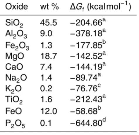
mineral dissolution. Chemical weathering in the model is based on the central assump-tion that dissoluassump-tion equilibrium is reached between the rock minerals and percolating water (Kirkby, 1977, 1985). In the model, water acts directly on the elemental oxides of the parent material rather than on rock minerals. The oxide composition and density of the bedrock provides the intial conditions for the modelled weathering process.

20

The simulated percolation of rainfall through the profile provides the mechanism and rate for losses of dissolved ions from the soil layers. The modelled soil may deepen as a result of steadily increasing percolation through the profile resulting from the increas-ing pore space which is created by the leachincreas-ing of dissolved rock oxides and also by the redistribution of soil by bioturbation and from direct removal by vegetation.

25

(6)

so-BGD

11, 5811–5868, 2014

Title Page

Tables Figures

◭ ◮

Back Close

Full Screen / Esc

Discussion

P

a

per

|

D

iscussion

P

a

per

|

Discussion

P

a

per

|

Discuss

ion

P

a

per

lution, organic carbon and pore CO₂ concentration. The processes included in the

model are, chemical weathering of bedrock elements, percolation of rainwater, leach-ing of weatherleach-ing products, surface erosion, bioturbation, plant litter decomposition and

vertical transport, CO₂production and diffusion and nutrient cycling. As well as

chemi-cal weathering, other adopted processes from Kirkby (1985) include losses of solutes

5

via leaching, surface erosion, biological mixing and ionic diffusion. The model differs

by keeping the bedrock elements separate throughout model calculations. Keeping chemical elements separate allows us to explore more comprehensively the individual cycling and feedbacks of important elements. The model processes are detailed in the following sections.

10

2.1 Mineral weathering and leaching

2.1.1 Equilibrium reactions

As already indicated, the model assumes that dissolution equilibrium is reached be-tween the rock oxides and the percolating waters. Although a simplistic assumption, as a first order approximation, this is preferable to a formulation using kinetic dissolution

15

equations which are particularly difficult to constrain due to the requirement of reactive

mineral surface areas. Studies have also shown that the unknowns associated with kinetic reactions are very large, with weathering rates of minerals such as plagioclase behaving closer to equilibrium predictions in natural systems than to kinetic rates de-rived from experimental studies (White et al., 2001, 2008). The methods of calculating

20

the equilibrium composition and thus the dissolution of rock oxides and subsequent pH of the soil solution are derived from Kirkby (1977) and Garrels and Christ (1965) and an

example taken from Kirkby (1977) for SiO₂is shown in the Appendix. The concentration

of H+in solution can be calculated by balancing the charge of the solution. Many of the

anions present in a soil solution result from the reactions with dissolved CO2. These

25

anions are calculated using the partial pressure of CO₂ in the soil air. The dominant

(7)

BGD

11, 5811–5868, 2014

Title Page

Tables Figures

◭ ◮

Back Close

Full Screen / Esc

Discussion

P

a

per

|

D

iscussion

P

a

per

|

Discussion

P

a

per

|

Discuss

ion

P

a

per

|

equation for our modelled soil solution is thus

[H+]+[Al(OH)+₂]+3[Al3+]+[Na+]+[K+]+2[Ca2+]+2[Mg2+]+3[Fe3+]+2[Fe2+]=

[HCO−

3]+[OH

−

]+2[CO2−

3 ]+[Al(OH)

−

4]+[H3SiO

−

4]+2[HPO

2−

4 ]

(1)

from which [H+] is calculated using a bisection method. The pH of the soil solution is

thus determined by the partial pressure of CO2in the soil and dissolved ion

concentra-5

tions.

The model assumes that the behaviour of the elemental oxides depends only on their relative composition in the bedrock. However, these oxides are not usually present on their own, but are instead constituents of more complex silicate minerals. This will alter the solubility of the individual oxides and to account for this Kirkby (1977) proposed

10

a correction term for the Gibbs free energy change of formation (∆Gf) of each oxide.

This correction term is determined by calculating the difference between the Gibbs free

energy change of formation of the silicate minerals and the sum of the free energies of

their constituent oxides. This difference is the formational free energy for the compound

and is shared between the oxides to give thee_ffective Gibbs free energy change of

15

formation (∆G′

f). In this study a set of likely minerals is calculated from the weight

percent of oxides in the parent rock and these are then used to find the correction factor. In order to determine the mineral assemblage of a rock from bulk chemical

analysis a mineral norm is calculated. The norm is a set ofidealised minerals that are

calculated from the known composition of oxides in a rock. The method of calculating

20

the minerals likely present is detailed in the Appendix.

2.1.2 Percolation and leaching

Percolation

The rate of water flowing through each soil layer is regulated by the amount of pore space available in that layer. In the early stages of soil formation this is dependent only

(8)

BGD

11, 5811–5868, 2014

Title Page

Tables Figures

◭ ◮

Back Close

Full Screen / Esc

Discussion

P

a

per

|

D

iscussion

P

a

per

|

Discussion

P

a

per

|

Discuss

ion

P

a

per

upon the porosity of the bedrock, however, over time, the losses due to leaching

in-crease this porosity. The pore space is expressed as a fraction of soil volume (m3m−3)

and is derived from the proportionp of original parent material remaining in the

pro-file, where p=1 for unweathered bedrock andp=0 for complete loss of the original

material. The total soil deficitwbelow depthzis calculated as

5

w(z)₌ z Z

∞

(1−p)dz (2)

and has the dimension of length. The coordinate system is chosen such thatz is

posi-tive in the downward direction.

A simple vertical flow through the profile is assumed, with sub-surface flow resulting

10

from the vertical variation in pore space. The percolation of water,F, at depthz is

F(z)−F₀=K w(z) (3)

whereF0 is the rate of percolation allowed through the bedrock andK is a site

spe-cific parameter related to hydraulic conductivity and slope gradient. Because F(z) is

15

the maximum rate of percolation, effectively occuring percolation is whichever is

low-est, the maximum rate of percolation or the rate of precipitation minus the cumulative

evaptranspiration from the soil surface to depthz.

Evapotranspiration

The process of evapotranspiration removes water from the soil profile. Here we

calcu-20

late total actual evapotranspiration (ET) as the minimum of potential evapotranspiration

(E∗

T) and mean annual precipitation (PA):

ET=min[E

∗

T,PA]. (4)

Although simple, the formulation still permits the model to operate under water

25

stressed conditions.E∗

(9)

BGD

11, 5811–5868, 2014

Title Page

Tables Figures

◭ ◮

Back Close

Full Screen / Esc

Discussion

P

a

per

|

D

iscussion

P

a

per

|

Discussion

P

a

per

|

Discuss

ion

P

a

per

|

model (Hargreaves and Samani, 1985) (see Appendix). This method is chosen be-cause it requires only a small amount of climate data (temperature) for any specific

location. The allocation of water loss by evapotranspiration to the different soil layers

is determined by the distribution of roots through the soil profile, these are assumed to decline exponentially with increasing soil depth (Jackson et al., 1996). The e-folding

5

rooting scale depth iszrso that the rate of evapotranspiration,E, at depthzis

E(z)=ET

zr exp

−z

zr . (5)

Rainfall minus cumulative evapotranspiration at depthzplaces a limit on the amount of

water available for percolation:

10

Ec(z)=ET(1−exp −z

z_r₎ ₍₆₎

whereEc(z) is the cumulative evapotranspiration from the surface down to depthz.

Val-ues forzr can be obtained from the rooting distributions compiled for different biomes

by Jackson et al. (1996). When the modelled soil is shallow, the rooting depth and

sub-15

sequent vertical distribution of evapotranspiration is limited by the soil depth. Rooting

depth, dr, is the depth which contains a fraction, f, of the total root mass (Arora and

Boer, 2003) and can be calculated by

dr=−ln(1−f)zr. (7)

20

If we term rooting depth as the depth above which 95 % of the total root biomass is

contained, following Arora and Boer (2003) we usef =0.9502 to aid simplicity, so that

dr=−ln(1−0.9502)zr=3zr (8)

Whendris greater than the soil depth in either the early stages of soil development or

25

in shallow soils, the above value ofzris adjusted so that dr equals soil depth. This will

(10)

BGD

11, 5811–5868, 2014

Title Page

Tables Figures

◭ ◮

Back Close

Full Screen / Esc

Discussion

P

a

per

|

D

iscussion

P

a

per

|

Discussion

P

a

per

|

Discuss

ion

P

a

per

Leaching

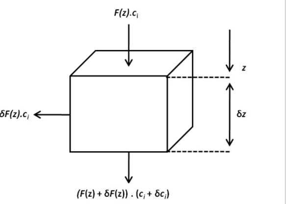
Loss of solutes from the profile can be calculated by mass balance (Fig. 1). The amount of solute carried into a soil volume at depthz by percolating water isF(z)c_i, wherec_i

(g m−3

) is the concentration of ion i in solution. The amount of solute lost from the

volume element by diversion due to sub-surface flow isδF(z)ci and due to percolation

5

outflow (F(z)+δF(z))(c_i+δc_i), thus

−δm_iδz=[−(δF)c_i−F c_i+(F+δF)(c_i+δc_i)]δt (9)

wheremi is the mass change of oxidei at depthz during timeδt. Neglecting second

order terms this reduces to

10 ∂m_i

∂t =−F(z) ∂c_i

∂z . (10)

The proportion, p_i, of oxide i remaining is then calculated from the original bedrock

density and the loss of mass from leaching

pt+1

i =p

t i−

mi

mi(t=0)

(11)

15

wherem_i(t=0) is the mass of elementi in the original parent material (ρbedrock×wt%

ofi).

2.2 Ionic di_ffusion

The ions released into solution from weathering can diffuse from regions of higher to

20

lower concentrations according to

∂c_i ∂t =

∂ ∂z

DI(z) ∂c_i

∂z

(12)

where DI is the diffusion coefficient of the ions which for current purposes we keep

fixed for all elements. This process is most important at the weathering front where ion

25

(11)

BGD

11, 5811–5868, 2014

Title Page

Tables Figures

◭ ◮

Back Close

Full Screen / Esc

Discussion

P

a

per

|

D

iscussion

P

a

per

|

Discussion

P

a

per

|

Discuss

ion

P

a

per

|

2.3 Bioturbation

Bioturbation is the mixing and turnover of soil resulting from biological activity and is considered a major soil forming process (Gabet et al., 2003; Wilkinson and Humphreys,

2005; Yoo et al., 2005). Bioturbation is represented in the model as a di_ffusive process:

∂p_i ∂t =

∂ ∂z

D(z)∂pi

∂z

(13)

5

where p_i is the proportion of element i remaining in the profile at depth z and D

(m2yr−1

) is the diffusion coefficient. It is assumed that the mixing intensity will decline with depth due to the decrease in faunal activity with increasing soil depth (Humphreys and Field, 1998; Wilkinson and Humphreys, 2005; Johnson et al., 2014). In the model

10

this takes the form of an exponential relationship:

D(z)=D(0) exp−z/z_b

(14)

whereD(0) is the diffusion coefficient at the soil surface andz_b is the e-folding length scale for biological activity (m). The boundary conditions at the top and bottom of the

15

profile allow no mixing in or out so that

∂pi

∂z =0 (15)

atz=0 andz=Nz, where Nz is the total number of vertical layers in the model.

2.4 Surface erosion

20

Removal of soil from the surface by mechanical processes is modelled through a de-nudation rate,T (m yr−1

). Surface elevation, zs is lowered at a rate, dzs/dt, which is

(12)

BGD

11, 5811–5868, 2014

Title Page

Tables Figures

◭ ◮

Back Close

Full Screen / Esc

Discussion

P

a

per

|

D

iscussion

P

a

per

|

Discussion

P

a

per

|

Discuss

ion

P

a

per

orp(z=1). In the model this lowering process shifts soil properties (or proportion of

substance remaining,p) up the soil profile and thus

p(z−δz,t+δt)=p(z,t) (16)

and

5

∂p

∂z(−δz)+ ∂p

∂tδt=0 (17)

or finally

∂p ∂t =

∂p ∂z

δz δt =

∂p ∂z

T

p_s. (18)

10

Cosmogenic nuclides such as in-situ10Be have provided measures of surface erosion

for hillslope soils where soil thickness is assumed to be at steady-state and thus rates of soil production from bedrock balance rates of loss due to surface erosion. Erosion

rates calculated from these studies lie in the range of 10 to 100 m M yr−1

(Wilkinson and Humphreys, 2005).

15

2.5 Organic carbon and CO2

2.5.1 Carbon fluxes, decomposition and mixing

To estimate carbon input into the soil we assume that vegetation cover is at steady-state, with new carbon production equal to the losses from litterfall and root senes-cence. For this first presentation and evaluation of the model we simply assume a time

20

invariant climate and annual net productivity (NP) (kg C m

−2

yr−1

). The carbon is

as-signed to four different pools which are defined by the stability or turnover time of the

(13)

BGD

11, 5811–5868, 2014

Title Page

Tables Figures

◭ ◮

Back Close

Full Screen / Esc

Discussion

P

a

per

|

D

iscussion

P

a

per

|

Discussion

P

a

per

|

Discuss

ion

P

a

per

|

fine roots and coarse roots. The overall equation for the organic matter decomposition and mixing processes in the soil profile is

∂C_i

∂t =

∂ ∂z

D(z)∂Ci

∂z

−k_i(z)C_i+I_i(z) (19)

whereCi is the concentration of carbon (kg m

−3

) in pooli, the first term is the diffusive

5

mixing of carbon through the soil profile by biological activity,k is the decay coefficient (yr−1

) and I_i is the carbon entering the soil profile from either plant litter at the

sur-face or from root litter which is distributed throughout the profile. The decay coefficient

may remain constant with depth or decrease with increasing soil depth as observed in soil carbon studies using carbon isotopes (Veldkamp, 1994; Trumbore et al., 1995;

10

Van Dam et al., 1997). For this study it is assumed that the decay rate, k, declines

exponentially with increasing soil depth. For the fine and coarse litter,I provides a top

boundary condition flux equal toα_iNP whereαi is the proportion of carbon production

assigned to pool i. For both fine and coarse roots the input of carbon is distributed

vertically throughout the profile according to

15

I(z)=αiNP

zr exp

−z

z_r _. ₍₂₀₎

Because of the much shorter timescale that these carbon dynamics operate on, we

assume a steady-state carbon profile and hence solve Eq. (19) for ∂C/∂t=0 and

boundary conditions of∂C_∂z =0 at the bottom and a top boundary condition equal to the

20

flux of carbon entering from the above litter. The carbon is not subject to the modelled

surface erosion, however, given the very different timescales of the two processes this

seems a reasonable simplification. A limitation of this carbon scheme is that biomass is present from the start of soil evolution rather than vegetation productivity evolving with the developing soil profile. This may result in an unrealistic vegetation enhanced

25

(14)

BGD

11, 5811–5868, 2014

Title Page

Tables Figures

◭ ◮

Back Close

Full Screen / Esc

Discussion

P

a

per

|

D

iscussion

P

a

per

|

Discussion

P

a

per

|

Discuss

ion

P

a

per

2.5.2 CO2production and diffusion

Gases in soil are transported in either the pore space or in solution. Here we assume

that the CO₂ produced from root respiration and from the above decomposition

pro-cess is transported through the profile by gaseous diffusion only. This is modelled as

a diffusion scheme:

5

∂C_g

∂t =

∂

∂z Dc(z) ∂C_g

∂z

!

+S(z)+Rc(z) (21)

whereC_gis the concentration of CO2(kg m

−3

soil air),Dc(z) is the diffusion coefficient of CO2in soil (m

2

s−1) at depthz,S is the CO2production rate (kg m

−₃

s−1) (calculated

byPn

i=1ki(z)Ci(z), wherenis the total number of carbon pools (4 in this case)) andRc

10

is the production of CO₂from root respiration which is assigned from the literature and

distributed throughout the profile following the same exponential function as for root carbon turnover. The effective diffusion coefficient in soil air is lower than that for bulk air due to both the smaller volumes of air filled pore space and the tortuosity introduced

by soil pores. The diffusion coefficient for CO2 is taken from Jones (1992), Dc=14.7

15

(mm2s−1

) for 20◦

C. To account for tortuosity a more realistic diffusion coefficient for soil air (Ds) is calculated using the following relationship of Penman (1940) (Hillel, 2004, pg. 204).

Ds(z) Dc

=0.66fa(z) (22)

20

wherefa is the fraction of air-filled space, in the model this is equal to 1−p(z). 0.66

represents the tortuosity coefficient, which means that the straight line path is

(15)

BGD

11, 5811–5868, 2014

Title Page

Tables Figures

◭ ◮

Back Close

Full Screen / Esc

Discussion

P

a

per

|

D

iscussion

P

a

per

|

Discussion

P

a

per

|

Discuss

ion

P

a

per

|

diffusive path will decrease. The CO₂profile is also modelled at steady-state so that

∂Cg

∂t =0 (23)

The top boundary condition is equal to the atmospheric concentration of CO2and the

bottom boundary condition allows no mixing out of the profile. This modelled partial

5

pressure of CO2 replaces the atmospheric CO2 concentration used in the carbonate

equations of the dissolution model and thus changes the charge balance of Eq. (1), influencing the pH of the soil solution and solubilities of the rock oxides.

2.6 Nutrient cycling

Nutrient concentrations in vegetation depend on a number of factors such as the

10

species of plant, the climate and the nutrient status of the soil. As a simplification, it is assumed in the model that the nutrients taken up and those re-entering the soil from plant litter and root turnover have fixed stoichiometric ratios. McGroddy et al. (2004) have found that within forest biomes, foliar C : N : P ratios are reasonably well constrained, with C : N ratios in litter globally similar.

15

We use the optimum stoichiometric nutrients ratios calculated by Linder (1995) for deciduous plants. For the following elements N : P : K : Ca : Mg : Fe these are 100 : 10 : 35 : 2.5 : 4 : 0.2. Nutrient concentrations are calculated assuming a fixed proportion of

biomass is made up of nutrients and a fixed relationship between NP and biomass

production (biomass is double the mass of carbon). The nutrients are released into

so-20

lution at the soil surface (g m−2yr−1) from the fine litter pool and provide a flux surface boundary condition in the solute transport equation (Eq. 10). The nutrients from fine root turnover are released into solution obeying the exponential decline in root distri-bution with depth. Although obviously not completely realistic, it has been observed that nutrients are readily lost from litter in the earlier stages of decomposition (Berg

25

(16)

BGD

11, 5811–5868, 2014

Title Page

Tables Figures

◭ ◮

Back Close

Full Screen / Esc

Discussion

P

a

per

|

D

iscussion

P

a

per

|

Discussion

P

a

per

|

Discuss

ion

P

a

per

Nutrients are then taken up from solution by the vegetation or leached from the system. Nutrient uptake from the soil profile is passive and controlled by the rate of evapotranspiration from each soil layer, the concentration of ions in solution in that layer and the rate of uptake required by the vegetation i.e. the fraction of biomass

production calculated fromNP. This process is represented by the second term in an

5

updated form of Eq. (10):

∂m_i

∂t =−F(z) ∂c_i

∂z − ∂Ec

∂z cni(z)+Rni(z). (24)

wherec_nis the concentration of nutrienti in each layer (g m−3

). Totalc_n_i is calculated by integrating∂Ec

∂zcni successively over each soil layer until the required annual uptake

10

of nutrients is reached (i.e. when total uptake of nutrientiequals the nutrient production

calculated from biomass production and hence turnover for the steady-state condition).

Rni is the concentration of nutrienti returned from fine root turnover (g m

−3

yr−1

). When

the nutrient uptake from a layer is greater than cn×∆t, uptake is set to cn/∆t. We

know that plants can interact directly with soil minerals for nutrients, however, the main

15

source of nutrients is likely the soil solution (Lucas, 2001) and this simple mechanism of nutrient uptake is employed for the first attempt at modelling long-term, plant-soil interactions.

3 Model solution and parameters

The model partial differential equations are solved numerically by finite-difference

20

schemes. The leaching and denudation equations are solved by an upwind scheme

(Morton and Mayers, 2005) and the diffusion equations by the semi-implicit

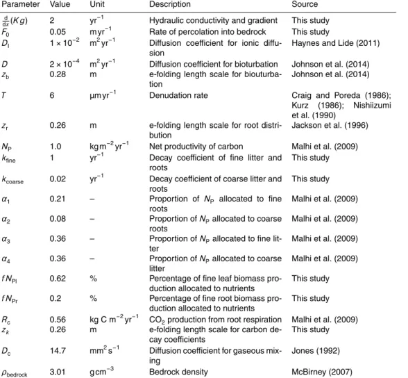
Crank-Nicholson scheme (Morton and Mayers, 2005). The parameters used in the model runs in the following section are shown in Table 1. The values are selected as being the most appropriate from the literature, they are not constrained for one particular site.

(17)

BGD

11, 5811–5868, 2014

Title Page

Tables Figures

◭ ◮

Back Close

Full Screen / Esc

Discussion

P

a

per

|

D

iscussion

P

a

per

|

Discussion

P

a

per

|

Discuss

ion

P

a

per

|

4 Model behaviour

In this section to permit easier interpretation of our model predictions we follow a hi-erarchial procedure. This involves first running the model in it’s most basic form and adding an additional process for each subsequent run. We can then get a clear sense of how each of the important processes influences the modelled soil properties and

5

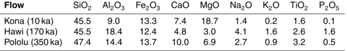
thus understand their importance in soil evolution within this modelling framework. In the following simulations the oxide composition of the model bedrock is a basalt taken from the study of a Hawaiian soil chronosequence (Porder and Chadwick, 2009) (Table 2, Kona flow). For the purpose of this study the model is run first with only oxide weathering and leaching as the active processes. Other processes are then added

suc-10

cessively in the order of surface erosion, bioturbation, organic carbon decomposition and nutrient cycling. For the simulations that follow, the profile is discretised into 10 cm deep layers and the total number of layers is chosen so that the total profile depth is greater than that reached by the weathering front during the simulation. The model timestep is 0.1 year. Unless stated otherwise the model is run with the parameters

15

in Table 1, and a mean annual temperature and precipitation of 20◦

C and 1.7 m yr−1

respectively.

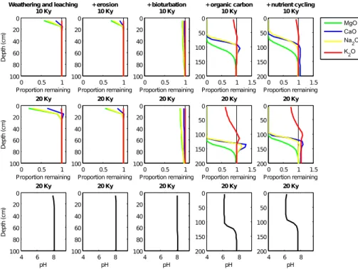
The developmental state of the modelled soil profile is quantified as the proportion of each oxide remaining in the soil layers relative to that of the parent material. Values lower than one represent a relative loss from the profile compared to the inital unaltered

20

bedrock material and values greater than one relative enrichment. A value equal to one indicates zero mobility.

4.1 Dissolution and leaching

With chemical weathering and leaching as the only active processes, we observe losses of the most souble oxides in only the top 20 cm of the soil profile (Fig. 2, first

25

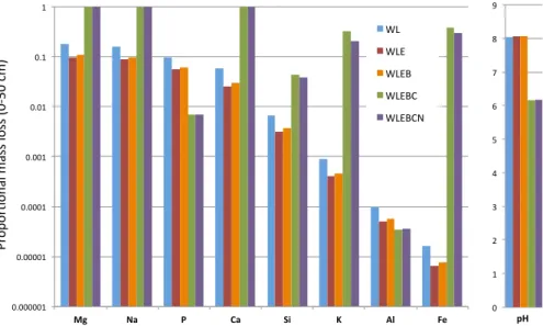
column). The sequence of losses for the basic oxides is MgO>Na₂O>CaO≫K₂O

(18)

ob-BGD

11, 5811–5868, 2014

Title Page

Tables Figures

◭ ◮

Back Close

Full Screen / Esc

Discussion

P

a

per

|

D

iscussion

P

a

per

|

Discussion

P

a

per

|

Discuss

ion

P

a

per

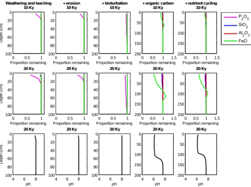
serve some depletion of P₂O₅ and SiO₂ but very minimal losses of FeO and Al₂O₃

(Fig. 3, first column and Fig. 4). The solubility of iron increases at lower pH values and Fig. 4 demonstrates the much greater losses of Fe when all processes are included

in the model simulation and soil pH has lowered from approximately 8 to 6. Al₂O₃ on

the other hand displays reduced losses in the full simulation and this is attributed to

5

aluminium being most soluble in either very alkaline or acidic solutions. At this stage the model displays very early signs of horizonisation, with a depleted top (or A) hori-zon and a slightly enriched saprolite (or B) horihori-zon. Enrichment or deposition of the most soluble oxides at the bottom of the weathering front occurs when saturated solu-tion from the layers above percolates into a bedrock layer with lower equilibrium solute

10

concentrations. At this most elementary stage of the model the weathering sequence of basic oxides displays similar weathering sequences to other studies. For example

Busacca and Singer (1989) observe a mobility sequence of Mg≫Na>Ca>K from

alluvium deposits in California and White et al. (2008) observe a weathering sequence of Mg>Ca>Na>K in marine terraces also in California. For the three basic oxides

15

found in the feldspar family of minerals, CaO, Na2O and K2O, the modelled sequence

of losses follow an expected trend associated with the lower solubility of K-feldspar (or orthoclase) compared to plagioclase which incorporates the endmembers anorthite and albite (Nesbitt and Young, 1984; White et al., 2001, 2008). Importantly, White et al. (2008) calculate that the pore waters of their chronosequence rapidly reach feldspar

20

thermodynamic saturation and so the weathering velocity of Ca, Na and K is controlled by this thermodynamic state, the rate of which is determined by the flux of water, this being the weathering mechanism of this model. White et al. (2008) also found that the weathering of plagioclase is non-stoichiometric, i.e. there is selective removal of Ca over Na from plagioclase in their marine terraces. Thus the solubility of the oxides act

25

independently, indicating that so far the dissolution and leaching of mineral oxides in this model is conceptually realistic.

(19)

under-BGD

11, 5811–5868, 2014

Title Page

Tables Figures

◭ ◮

Back Close

Full Screen / Esc

Discussion

P

a

per

|

D

iscussion

P

a

per

|

Discussion

P

a

per

|

Discuss

ion

P

a

per

|

standing of the sequence of minerals formed across gradients of weathering intensities. The modelled weathering sequence thus predicts the commonly predicted weathering pathway of a shift from predominantly silicate minerals such as the Mg, Ca and K feldspar family to the secondary Fe and Si containing clays such as vermiculite and montmorillonite, through to the Al and Si containing clay mineral kaolinite present in

5

weathered soils. Eventually, in very weathered soils Al sesquioxides such as gibbsite dominate (Tardy et al., 1973).

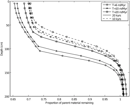
The predictions based on chemical weathering and leaching processes alone demonstrate (i) an expected weathering sequence of oxide losses, (ii) an increase in the depth of the weathering front with increasing time since the intiation of soil

de-10

velopment, (iii) very shallow soil profiles in the absence of any physical weathering or biological activity and (iv) evidence of horizonization.

4.2 Surface erosion

The modelled process of surface erosion acts by shifting the simulated soil properties towards the soil surface, whilst removing those in the surface layers (Figs. 2 and 3,

15

second column and Fig. 5). Erosion plays a larger role in older, more depleted soils. This is demonstrated when all processes are included in the model simulations (Fig. 5). The more weathered and depleted in original material the surface layer is, the greater the reduction in surface elevation, with a shallower profile then ensuing. Thus over long timescales surface erosion becomes an increasingly important process in the soil

20

evolution model. If the rate of soil deepening becomes equivalent to the rate of surface denudation, soil thickness naturally reaches a steady-state.

4.3 Bioturbation

Parameterised here as a diffusion process, bioturbation smoothes the oxide

distribu-tions in the surface layers (Figs. 2 and 3, third column) allowing the upward mixing of

25

(20)

BGD

11, 5811–5868, 2014

Title Page

Tables Figures

◭ ◮

Back Close

Full Screen / Esc

Discussion

P

a

per

|

D

iscussion

P

a

per

|

Discussion

P

a

per

|

Discuss

ion

P

a

per

results in retention of mineral oxides in the surface layers (Fig. 4). Bioturbation acts to deepen the soil by removing material from deeper in the profile and mixing it into the upper layers. Bioturbation thus influences both the composition of the soil layers and the rate of soil production from bedrock.

4.4 Vegetation interactions

5

The modelled vegetation interacts with the soil via three processes: by the uptake of

water from the soil, by increasing soil acidity through the production of CO2from root

respiration and litter decomposition, and through the cycling and retention of nutrients. Vegetation thus potentially plays an important role in modelled soil development.

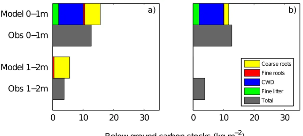
At steady-state the highest carbon stocks are in the surface layers (Fig. 6). For the

10

control run when the rate of decomposition,k, declines with increasing soil depth, the

carbon persists in the deeper soil layers (1–2 m) (Fig. 6a), whereas, when the decay rate of the carbon pools remains constant with depth, organic carbon is absent below 1 m (Fig. 6b). The comparisons with observed below-ground carbon concentrations suggest that the decreasing decay rate with increasing soil depth is perhaps the most

15

realistic formulation (Fig. 6).

The addition of organic matter to the soil accelerates the weathering of all but the most insoluble oxides (Figs. 2 and 3, column 4). When carbon biomass is absent

from the model simulation, soil development progresses slowly, CO2 concentrations

are equal to atmospheric concentrations, and pH remains above 7. When organic

car-20

bon is included in the model simulations pH decreases from∼8 in the surface layers

to∼6 after 20 thousand years of soil development (Fig. 2, column 4 and Fig. 4).

This decrease in pH and increase in leaching losses is a result of the higher

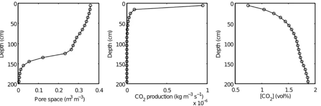
concen-trations of soil CO₂ (Fig. 7). CO₂ concentrations increase with increasing soil depth,

reaching over 100 times atmospheric levels in the early stages of soil development

25

when pore space is low (Fig. 8). The CO2 concentrations in the soil profile decrease

over time from very high initial concentrations due to the creation of pore spaces in the

(21)

BGD

11, 5811–5868, 2014

Title Page

Tables Figures

◭ ◮

Back Close

Full Screen / Esc

Discussion

P

a

per

|

D

iscussion

P

a

per

|

Discussion

P

a

per

|

Discuss

ion

P

a

per

|

concentrations are highest when the carbon productivity is highest (Fig. 8) because of the greater inputs of organic carbon into the soil. Deeper root profiles result in higher

soil CO2concentrations at deep depths (Fig. 8c). This is due to the higher inputs from

root decomposition and root turnover at these depths and lower tortuosity which hin-ders CO2diffusion into and out of the surface layers. For this simulation the flux of CO2

5

out of the soil profile is within the ranges observed in studies of Hawaiian tropical forest soils (Fig. 9).

The addition of nutrient cycling into the simulation results in some retention of the oxides in the surface layers (Figs. 2 and 3, column 5), a trend also noted in the soil-nutrient studies of Jobbágy and Jackson (2001); Lucas (2001) and Porder and

Chad-10

wick (2009). However, in older or very wet soils the e_ffect of plants on nutrient retention

may be diminshed due to the overriding effect of leaching losses as found by Porder

and Chadwick (2009). In the model the return of basic ions in solution from litter decom-position alters the equilibrium status of the solution and slows the rate of dissolution.

This step-wise approach of including processes in the model framework has

demon-15

strated the important role vegetation plays throughout modelled pedogenesis and thus highlights the possible significant influence that vegetation may have on the long-term carbon cycle and hence climate.

5 Comparison of model predictions with observations

To assess the ability of the model to reproduce real soil profiles we compare the model

20

predictions with data from in-situ soil profiles from soil chronosequences. Due to the slow nature of pedogenesis it is impossible to directly observe soil changes over these very long timescales. Instead we make use of chronosequences. These are series of soils which differ in the age of soil initiation but other factors of soil formation such as parent material, climate and topography remain constant. It is thus assumed that any

25

di_fferences in soil properties are related only to the di_fferences in the age of the soil

(22)

BGD

11, 5811–5868, 2014

Title Page

Tables Figures

◭ ◮

Back Close

Full Screen / Esc

Discussion

P

a

per

|

D

iscussion

P

a

per

|

Discussion

P

a

per

|

Discuss

ion

P

a

per

Hawaiian soil chronsequence data published by Porder et al. (2007) and Porder and Chadwick (2009), are used for comparison here. The soils have developed on volcanic lava flows on the island of Hawaii, and thus have a parent material of relatively uni-form composition (Table 2). Because of the wide range in eruption ages, soils from the Hawaiian island chain have been utilised in a number of studies looking at the

in-5

teractions between soil age, weathering and nutrients (Vitousek et al., 1994; Vitousek and Farrington, 1997; Chadwick et al., 1999; Hedin et al., 2003; Porder et al., 2007; Porder and Chadwick, 2009). Porder et al. (2007) sampled soils on three lava flows aged 10 ka, 170 ka and 350 ka, each spanning a topographic gradient and resulting rainfall gradient. Mean annual precipitation (P_A) varies from 0.57 m yr−1

to 2.5 m yr−1

,

10

the highest rates of precipitation are found at the highest elevations. Mean annual

tem-perature (TA) increases from 16

◦

C at these higher and wetter elevations to 24◦

C at the lower altitudes. Consequently the sites receiving the lowest rainfall have the

high-est temperatures and are thus subject to the highhigh-estET, resulting in a negative water

balance (Chadwick et al., 2003). It is important to note that the rainfall gradient has

15

not always been this strong during the evolution of the soil profiles, this is a result of glacial periods and changes in the elevation of the trade wind inversion (Hotchkiss et al., 2000). The sites at the wet, higher elevations may have received 50 % less pre-cipitation during most of their development, however, the temperatures during these drier glacial periods were also cooler, thus probably reducing the water lost from the

20

profile by evapotranspiration.

The model is compared with the driest and wettest sites from each flow and an in-termediate rainfall site. The following model parameters are modified from those in Table 1 to suit the Hawaiian sites. The monthly minimum and maximum and mean

temperatures needed to calculateET using the Hargreaves equation are taken from

25

the Western Regional Climate Center (http://www.wrcc.dri.edu/). The site closest to

the Kona lava flows is used and the temperatures were adjusted toTA of 16

◦

C, 20◦C

and 24◦

C for the low, medium and wet rainfall sites respectively. The estimatedE∗

T

(23)

BGD

11, 5811–5868, 2014

Title Page

Tables Figures

◭ ◮

Back Close

Full Screen / Esc

Discussion

P

a

per

|

D

iscussion

P

a

per

|

Discussion

P

a

per

|

Discuss

ion

P

a

per

|

values for each site by relatingET to productivity using a water use efficiency (WUE)

term. The WUE of a plant is the unit of carbon fixed per unit of water transpired.

As-signing a WUE of 1 kg m−3

we estimate carbon productivity (NP) values of 0.3, 0.53

and 0.48 kg m−2

yr−1

for each of the sites respectively, replicating the observed trend

for Hawaiian vegetation of increasingNPwithPA up to approximately 2 m yr

−1

, decling

5

for further increaes in rainfall (Schuur and Matson, 2001; Austin, 2002). However, we are aware that the mechanisms behind this relationship are not the same. The de-crease in the model productivity is due to decreasing evapotranspiration associated

with decreasingPA, whereas, the changes in the observations are thought to be due

to decreased N availability. The vertical root depth scale (z_r) is 0.26 m, the value

es-10

timated for tropical evergreen forests (Jackson et al., 1996). The bedrock oxide com-positions used in the model runs are shown in Table 2. The erosion rate is set to 10 m Myr−1

because even though the soils sampled are not thought to have experi-enced high rates of erosion (Porder et al., 2007), even stable soils often experience

erosion rates greater than 5 m M yr−1(von Blackenburg, 2005) and values in the range

15

of 7.7 to 12 m Myr−1

were calculated for basalts on the lip of Hawaiian volcano craters (Craig and Poreda, 1986; Kurz, 1986; Nishiizumi et al., 1990). Townsend et al. (1995) found that the turnover times of the intermediate carbon pool in Hawaii soils double with a 10◦

C decrease inTA. It is unclear whether this increase in decomposition with

in-creasing temperature follows a linear or exponential trend but here we assume a simple

20

linear function of decomposition with mean annual temperature using the values

ob-served by Townsend et al. (1995) to calculate the decomposition rate (k) of the coarse

roots and coarse wood:

kcoarse=0.0026.TA−0.02 (25)

25

The decomposition rates (k) of the fast carbon pools remain the same as in Table 1.

(24)

BGD

11, 5811–5868, 2014

Title Page

Tables Figures

◭ ◮

Back Close

Full Screen / Esc

Discussion

P

a

per

|

D

iscussion

P

a

per

|

Discussion

P

a

per

|

Discuss

ion

P

a

per

To determine the intensity of weathering of elements in a soil profile, element concen-trations are commonly compared with those in unweathered bedrock and normalised to an immobile element such as zirconium (Zr) to give the fraction of the particular el-ement remaining relative to bedrock (Brimhall and Dietrich, 1987) (See the Appendix for a description of this method). For these Hawaiian soils Porder et al. (2007) used

5

Niobium (Nb) as the immobile element. This provides values which can be directly compared with output from the model.

It is recognised that soils are complex systems and display a great deal of hetero-geneity across even very small spatial scales. Nevertheless, we assume here that over these pedogenic timescales the soils sampled at each of these sites have been subject

10

to the same soil-vegetation interactions.

Figure 10 illustrates the performance of the model for the three different rates of

annual precipitation on the young 10 ka lava flow for a selection of elements. The simulations of Ca and Na in the model are most realistic, followed by Mg, and then K and P. The model captures the slower rate of weathering losses in the driest site and

15

higher rates in the intermediate and high rainfall sites. Mg, Ca and Na display very similar distributions of depletion in these Hawaiin soils, whereas the relative vertical

distribution of Mg depletion differs from that of Ca and Na in the model. Modelled Mg

weathers to deeper depths than those observed in the intermediate rainfall sites (where

modelNPis highest), also weathering deeper than the other model elements. Modelled

20

K is particularly resistant to weathering compared with the observations. K is required by plants in larger amounts than Ca and Mg and is thus strongly cycled (Jobbágy and Jackson, 2001). The model results for K may thus highlight the importance of the active role of plants, mycorrhiza and faunal communities in mediating the release of this poorly mobile nutrient from minerals (Hutchens, 2009). The uptake of nutrients in the model is

25

controlled by the rate of evapotranspiration and concentrations of the nutrient in the soil solution, however, there are a number of other mechanisms by which plants can aquire nutrients (Hinsinger et al., 2009). For example, roots can actively induce the release

(25)

BGD

11, 5811–5868, 2014

Title Page

Tables Figures

◭ ◮

Back Close

Full Screen / Esc

Discussion

P

a

per

|

D

iscussion

P

a

per

|

Discussion

P

a

per

|

Discuss

ion

P

a

per

|

actively taking up K from solution plants can also shift the solution equilibrium thus promoting further dissolution (Hinsinger et al., 1993; Hinsinger and Jaillard, 1993). By altering the solubility of K in our model, we show that the missing process accelerates the weathering of K from minerals by a factor of approximately 50 (Fig. 11). Modelled P is even more immobile than K, however, the observations also exhibit little depletion

5

of P in these young profiles. The 10 ka flow is characterized by surface layers enriched in P and low amounts of P depletion in the deeper layers of the intermediate and wet sites. For the driest site (Porder and Chadwick, 2009) argue that the soils must receive additional P from exogenous sources. If this enrichment was due to cycling of the nutrient we would expect this surface enrichment to be balanced by depletion deeper

10

in the profile, which is not observed. Dust can be a significant source of P to Hawaiin soils (Chadwick et al., 1999), but for these young flows Porder and Chadwick (2009) suggest that the addition of fine organic matter from nearby surroundings may explain the additions. Without these external sources of P, the relative immobility of modelled P may be representative of these young soils.

15

For the 170 ka Hawi flow, both the Hawaiian and modelled soils have weathered much deeper in the intermediate and high rainfal sites compared with the younger 10 ka flow. The model captures the lower losses in the dry site relative to the wetter sites but does not replicate the more enriched surface layers (Fig. 12). The modelled Na and Ca profiles again match the observations most closely, reproducing the nearly

20

totally depleted profiles at the wetter sites and even matching the depth of weathering. The depth of the Mg weathering front, however, is still too deep and the modelled K and P profiles indicate that the modelled processes are still too resistent to weathering for these elements. It should be noted that Porder et al. (2007) estimate that additions of dust to the Hawi flow averages 30 % of the total mass lost from the profiles and most

25

of this dust is found in the top 30 cm which may obscure some of the weathering signal in these soils.

The 350 ka Pololu flow differs from the 10 ka and 170 ka flow by being underlain by

(26)

sur-BGD

11, 5811–5868, 2014

Title Page

Tables Figures

◭ ◮

Back Close

Full Screen / Esc

Discussion

P

a

per

|

D

iscussion

P

a

per

|

Discussion

P

a

per

|

Discuss

ion

P

a

per

faces and are less porous than the overlying, blocky lava flows. They therefore act as a barrier to weathering in these soils. By comparing the profiles of K with Na Porder and Chadwick (2009) show that even at this age, plants in the dry flow are still enriching the surface layers with nutrients but in the intermediate and high rainfall sites, leaching losses override any nutrient retention and the surface layers are depleted in nutrients.

5

Figure 13 shows that for the dry site the model displays general agreement with weath-ering depths and again Na shows the closest match to the observations followed by Ca and Mg with K and P still too immobile at this age. The slow rate of chemical weath-ering of these two elements in the model also means that any depleted signal in the surface layers will also be removed by surface erosion. For the intermediate and wet

10

rainfall sites the model captures the surface losses of Na, Ca and Mg, K is still is still too resistant in the intermediate site but agrees better at the wettest site. For this older soil, modelled P shows some signs of depletion but is still much more resistant than the observed profiles. In the Hawaiian soils P losses are correlated with Fe losses in the old and wet sites, Fe can bind with P and may drive the losses in these lower oxygen,

15

reducing soils (Porder and Chadwick, 2009), a process not represented in the model. The modelled profiles extend to nearly five metres for the two wetter sites whereas the observed profiles reach a maximum of 1.8 m because of the impermeable pahoehoe layer at this depth.

Figure 14 shows the comparisons between the observations and modelled pH

pro-20

files. Modelled pH agrees best with observations in the driest sites and for the inter-mediate aged, Hawi flow. Simulated pH is generally too high in the wetter sites which

could be because modelled Al₂O₃is very insoluble (Fig. 3) so Al3+ions in solution may

be lower.

These comparisons show that for all profiles modelled plant nutrients P and K are

25

(27)

BGD

11, 5811–5868, 2014

Title Page

Tables Figures

◭ ◮

Back Close

Full Screen / Esc

Discussion

P

a

per

|

D

iscussion

P

a

per

|

Discussion

P

a

per

|

Discuss

ion

P

a

per

|

uptake which the model is not reproducing realistically. The good agreement with Na, particulary in the intermediate rainfall sites where plants play an important role in nu-trient distributions suggests a good model understanding of the other soil processes included in the model and thus that the model will provide a reliable platform for further developing our understanding of nutrient dynamics.

5

6 Conclusions

This study has demonstrated that the soil evolution model presented is capable of re-producing realistic soil properties such as relative elemental losses, weathering depths,

pH profiles, organic carbon content and soil-pore CO2 concentrations. The model

re-quires 20 parameters, of which at least 13 are easily assigned from literature, plus

10

regional climate, bedrock data and simple thermodynamic constants to simulate soil genesis on a chosen parent material. The limited number of processes and the ease at which they can be both included and excluded from simulations makes the model behaviour easy to understand. This study has detailed how each of these model pro-cesses interacts with and influences the soil properties.

15

Comparisons of the model predictions with a Hawaiian soil chronosequences has highlighted the importance of vegetation in shaping soil profile evolution by increasing soil acidity and cycling nutrients. The good model agreement with the observations of Na, Mg and Ca which are less strongly cycled by vegetation, suggests that the model is realistically reproducing the other processes unrelated to nutrient cycling. These results

20

lend confidence to the model’s ability to quantify processes and feedbacks occuring during pedogenesis and to the valuable role it can play in understanding long-term biogeochemical cycles.

Minasny et al. (2008) highlight a number of criteria that a pedogenetic model should comply with, these are (1) the model should be based on physical laws (2) the model

25