Three-Dimensional Reconstruction of Non-Homogeneous
Dielectric Objects by the Coupled-Dipole Method
Amin Bassrei Universidade Federal da Bahia,
Instituto de F´ısica & Centro de Pesquisa em Geof´ısica e Geologia Campus Universit´ario de Ondina
40170-290 Salvador BA, Brazil
and Thierry J. Lemaire Universidade Estadual de Feira de Santana
Departamento de F´ısica
Av. Universit´aria, s/n, Campus Universit´ario, km 03, BR 116 44031-460 Feira de Santana BA, Brazil
Received on 9 February, 2006; revised version received on 5 November, 2006
In this paper we present an inversion procedure for electromagnetic scattering, based on the coupled-dipole method (CDM) combined with an inversion algorithm making use of the singular value decomposition pro-cedure associated with a regularization factor. This method permits to obtain images of non-homogeneous dielectric objects whose dimensions are comparable to the incident wavelength. The feasibility of this method is showed in two synthetic examples using the CDM with 257 and 515 dipoles, for spherical objects with a spherical inclusion. The method also works if the scattered electric field, which is the input data, is corrupted with Gaussian noise.
Keywords: Electromagnetic scattering; Coupled-dipole method; Inverse problems; Singular value decomposition; Regular-ization
I. INTRODUCTION
Electromagnetic scattering phenomena have been shown to be of great importance because of their various applications in many areas [1–4]. The ability of electromagnetic waves to penetrate into objects without making alterations of their structure is an important property and permits to obtain infor-mation about the studied scattering object, i.e., it is possible to make a non-destructive imaging analysis.
Several methods were developed to solve inverse electro-magnetic problems. Most of the methods dealing with mi-crowave imaging are based on the discretization of an integral equation for the electric field or the current density. This leads to a linear system of equations which is ill-posed and conse-quently the solution is not unique.
Recently, a new numerical technique [5] was introduced in order to obtain the complex refractive index of a homogeneous scattering object in the scope of active microwave imaging. The modeling of the scattering phenomenon is based on the well-known coupled-dipole method (CDM) [6, 7] and sim-ulations showed the feasibility of this technique even with corrupted data. In this paper are presented new results for non-homogeneous scattering objects with artificial data (noise free and also corrupted by noise), using the truncated singular value decomposition (SVD) method to make the data inver-sion. The method applied to non-homogeneous spheres shows a reasonable resolution to detect the inclusion.
This non invasive and non destructive technique is very use-ful to determine the dielectric properties of an object [4]. The input physical quantity of interest is the electric field and the searched characteristics of the object are the permittivity (gen-erally a function of space coordinates) and geometry. Our
ap-proach is based on the inversion of the CDM which permits to describe the scattered electric field. This inversion technique [5] using the CDM is shown to be efficient when applied to a homogeneous and isotropic scatterer of size parameter less than 10.0.
This inversion scheme is tested with synthetic data for sim-ple geometries of the scatterer, and noisy data are used to illus-trate its stability. The a priori information used in this model is the external shape of the studied object. This paper is orga-nized as follows. In Section II we briefly describe the CDM. In Section III, the inversion procedure is introduced and nu-merical results are given in Section IV. Section V is the con-clusion.
II. COUPLED-DIPOLE METHOD
The theoretical description of the scattering phenomenon is done with the well known CDM. The polarizability of each in-duced dipole located at the sites of a cubic lattice is given by the Clausius-Mossotti (or Lorentz-Lorenz) prescription [1]. We remind that the basic equation to be inverted is the re-lation between the measured scattered electric fieldEscat(ri) atri, and theNelectric dipolar momentspj,(j=1, ...,N)of the dipolar units, located atrj,
Escat(ri) =
∑
j=1,...,Nwhere the 3×3 complex matrixΠ(r)is given by [8] (for a time factor exp(−iωt)),
Π(r) =e ikr
r ½
k2(I−n⊗n) +1−ikr
r2 (3n⊗n−I)
¾
, (2)
“⊗” is the Kronecker product, and Iis the unit 3×3 matrix. The data to be inverted are the scattered electric fields, and the inversion output is the dipolar moment of each dipolar unit. This last quantity is used to obtain the polarizability of each dipolar unit and, consequently, the refractive index of each site of the cubic lattice. However, the Freedholm equation of first kind (1) is ill-conditioned making the inversion process not trivial.
III. DATA INVERSION
The inversion procedure is a 3-step algorithm. The first one leads to the inversion of a system of linear equations (1) ob-tained by writing the scattered field at each point where it is measured. The second step leads to the estimation of the po-larizability at each site of the lattice by use of the equation [5],
αi=kpik2/{(E0(ri) +
∑
j=1,...,N
j6=i
Escat,j(ri)).p∗i}, (3)
whereE0is the incident field. The last step leads to the
de-termination of the complex refractive index at each site from the Clausius-Mossotti formula. Let us notice that the main computational time is spent at the first step of the algorithm because of the large size of the matrix to be inverted.
As mentioned above, we will perform the inverse procedure by the SVD technique. Our basic equation here is
Escat=Πp, (4)
which is a linear transformation onp. If the vectorEscat de-scribes the observed actual output of the system, the problem is to “choose” the vector of model parametersp in order to minimize, in some sense, the difference between the observed
Escat and the prescribed output of the systemΠp. In order to solve the system of linear equations, we have first to invert the matrixΠ, obtaining the pseudo-inverseΠ+, then multiply the pseudo-inverse by the scattered field, obtaining finally the recovered vector of momentspestwhich permits the computa-tion of the refractive index.
The generalized inverse matrix is frequently used in inverse problems, and its solution has the minimum Euclidean norm. In this case the objective function to be minimized is
Φ(p) =pT·p+tT·(Escat−Πp), (5)
wheretis the vector of Lagrange multipliers. The minimiza-tion yields
p=ΠT(ΠΠT)−1E
scat. (6)
The above equation is equivalent to the so-called “pseudo-inverse” for underdetermined systems developed by [9] and later by [10]. One versatile way to calculate the pseudo-inverse is through SVD [11] where the square kernel matrix is expressed as
Π=UΣVT, (7)
whereU is the matrix which contains the orthonormalized eigenvectors ofΠΠT,Vthe orthonormalized eigenvectors of
ΠTΠand the matrixΣis formed by the singular values ofΠ. The pseudo-inverseΠ+will be given by
Π+=VΣ−1UT, (8)
whereΣ−1=(1/σ
ii),i=1, ...,k,and 1/σll=0, forl>k.
IV. NUMERICAL SIMULATIONS
In order to show the feasibility of this method, we present two synthetic examples where a non-homogeneous sphere with a spherical inclusion is described by 257 and by 515 dipoles. In both examples the refractive index of the homo-geneous background is 1.1 and the index of the inclusion is 1.4. The choice of this simple shape is not a limitation and the extension to other scatterer geometry is straightforward. In order to obtain the synthetic data to be inverted, which is the scattered electric field, we calculate the dipolar moments us-ing the CDM approach. Each dipole is associated with a vec-tor of six components: three components of the real dipolar moment, and three components of the imaginary one. Thus, in the inversion procedure, we have 6×257 = 1542 model parameters for the first example and 6×515 = 3090 for the second one.
The acquisition geometry is performed in two planes around the scatterer. Using standard notation for spherical coordinates, for one plane we haveφ=0 and for the other
φ=π/2. The angleθvaries from 0 toπ. For the first example one plane has 128 observation points and the other has 129, while for the second example one plane has 257 observation points and the other has 258. This means that for the first situ-ation there are 257 observsitu-ation points and for the second one there are 515 observation points.
Since the scattered electric field used as the input for the inverse procedure is also a complex vector, we have 6×257 = 1542 data parameters for the first example and 6×515 = 3090 for the second one. The number of data parameters is then equal to the number of model parameters, making the system determined although ill-posed. The matrixΠis then square, but this is not a limitation, that is, we could have more data parameters than model parameters, making the problem overdetermined, or the opposite situation, with more model parameters than data parameters, making the problem in this case underdetermined.
1e-16 1e-14 1e-12 1e-10 1e-08 1e-06 0.0001 0.01 1 100 10000 1e+06
0 200 400 600 800 1000 1200 1400
singular value amplitude
number of dipoles times 6
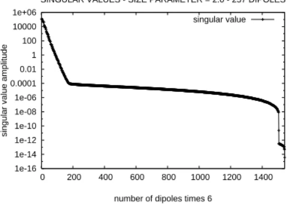
SINGULAR VALUES - SIZE PARAMETER = 2.0 - 257 DIPOLES
singular value
FIG. 1: Singular values of the 257 dipoles simulation (ka=2.0).
TABLE I: Simulation results for 257 dipoles.
β εrms(%) λbest εmrms(%) ε f ield
rms (%) εindexrms (%)
0.0 0.00 10−3 46.56 0.00 8.62
0.2 2.67 10+2 49.42 2.67 9.27
0.4 5.38 10+2 49.90 5.29 9.28
0.6 8.07 10+2 50.75 7.92 9.40
0.8 10.76 10+2 51.94 10.56 9.56
1.0 13.44 10+2 52.07 13.44 9.86
at(x1,y1,z1)with(kx1=0.4,ky1=0.4,kz1=0.4). The
sin-gular values can be seen in Fig. 1 for 257 dipoles example. The behavior of singular value decay was quite similar for the simulations with 515 dipoles.
The ill-posedness of the problem suggests us the need of some kind of regularization. We have employed the damped least squares approach, as proposed by [12] and [13]. Here the matrixΠTΠis damped with a positive constant, in order to stabilize the inversion. Other kinds of regularization can be applied like filtering the matrixΠTΠwith a second or fourth order derivative matrix as proposed by [14–18]. Let us notice that the choice of the regularization factorλis a problem by it-self. Several techniques have been suggested in the literature. Since the purpose of this work is not to explore this search for the optimum regularization factor, we have adopted the fol-lowing procedure: for each example, we used several noise levels, and for each noise level we performed 35 inversions, each one with a differentλ, computing the root mean square (rms) error for the data parameters and for the model parame-ters. The range forλwas rather wide, fromλmin=1×10⁻¹⁵ toλmax=1×10+19.
The results of the simulations are summarized in Tables I and II. Table I is for 257 dipoles and Table II for 515 dipoles. In each table the first column gives the value of noise factorβ
which is added to the scattered electric field(Escatf ree), so that
Escat=Escatf ree+β
∑
j=1,...,N(ranj Escatf ree,j)ej, (9)
whereranjis a sequence of random numbers within the range [0, 1].
The second column gives the noise estimateεrms, which is
TABLE II: Simulation results for 515 dipoles.
β εrms(%) λbest εmrms(%) ε f ield
rms (%) εindexrms (%)
0.0 0.00 10−3 48.69 0.00 9.28
0.2 2.80 10+2 50.43 2.78 9.76
0.4 5.61 10+2 50.96 5.56 9.90
0.6 8.42 10+2 51.85 8.34 10.08
0.8 11.22 10+2 53.08 11.12 10.36
1.0 14.03 10+2 54.64 13.88 10.75
the relative rms error betweenEscatandEscatf ree:
εrms= q
∑Ni=1[Escat(ri)−Escatf ree(ri)]2 q
∑Ni=1[E
f ree scat(ri)]2
×100 %.
As mentioned above for each noise level we run 35 inver-sions, where each simulation had a different regularization factorλ, used to compute the estimated moment vector:
pesti = (ΠTΠ+λITI)+ΠTEscat. (10)
The bestλ, that is, theλwhich provides the minimum rms error between the vector of true moment and the vector of estimated moment, is given in the third column. This relative rms error is denoted byεm
rms(see the fourth column in Tables I and II) and expressed by
εm rms=
q
∑Ni=1(ptruei −pesti )2 q
∑Ni=1(ptruei )2
×100 %.
Note that the value for the bestλis kept constant with different noise levels, not showing fluctuation.
We can compute once more the scattered field associated with the estimated moment vectors by applying the forward modeling procedure,
Ecalcscat=Πpest. (11)
In the tables, the fifth column gives the relative rms error be-tween the (observed) scattered electric field and the calculated scattered electric field, denoted byεrmsf ield:
εf ield rms =
q
∑Ni=1[Ecalcscat(ri)−Escat(ri)]2 q
∑Ni=1[Escat(ri)]2
×100 %.
The inversion output, pest, is used to calculate the polar-izabilityαest, which is then used to calculate the estimated refraction indexnest, with the Clausius-Mossotti formula. Fi-nally the last column in the tables shows the relative rms error between the true refraction index and the estimated one,
εindex rms =
q
∑Ni=1(ntruei −nesti )2 q
∑Ni=1(ntruei )2
TRUE MODEL
y
x
1.0 1.4
x
y
FIG. 2: True model with 257 dipoles,kz=0.0.
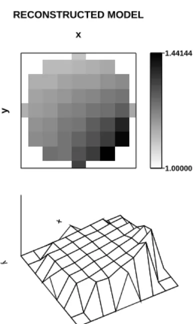
RECONSTRUCTED MODEL
y
x
1.00000 1.44144
x
y
FIG. 3: Simulation with 257 dipoles, forward modeling withka=
2.0,kz=0.00, inversion by SVD.
Due to space limitations we show only some results from the two examples. In each figure we show, for a given slice or projection, the 2–D image with gray scale as well as the contour map. Just the noise free results are showed in the fig-ures. A compilation of the results with all noise levels tested can be seen in the above tables. Also, only two projections are showed:kz=0.0, which is at the equator, andkz=0.75, which is located at 3/4 from the equator.
In the first example the sphere is formed by 257 dipoles. This means that at the equator the model has a diameter formed by 9 dipoles. The inclusion, with refraction index
TRUE MODEL
y
x
1.0 1.4
x
y
FIG. 4: True model with 257 dipoles,kz=0.75.
RECONSTRUCTED MODEL
y
x
1.00000 1.52152
x
y
FIG. 5: Simulation with 257 dipoles, forward modeling withka=
2.0,kz=0.75, inversion by SVD.
agree-TRUE MODEL
y
x
1.0 1.4
x
y
FIG. 6: True model with 515 dipoles,kz=0.00.
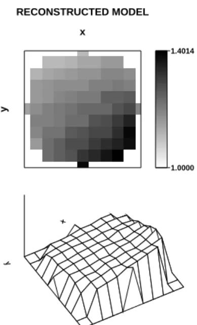
RECONSTRUCTED MODEL
y
x
1.0000 1.4014
x
y
FIG. 7: Simulation with 515 dipoles, forward modeling withka=
2.0,kz=0.00, inversion by SVD.
ment in relation to the location and intensity but a poor shape definition.
In the second example the sphere is formed by 515 dipoles, which implies that at the equator the model has a diameter formed by 11 dipoles. Again, the inclusion with refraction index equal to 1.4 is larger than the radius, with its maximum diameter at the equator formed by 7 dipoles. The true model forkz=0.0 is presented in Fig. 6, and the noise free inversion in Fig. 7. For thekz=0.75 projection, Fig. 8 shows the true model and Fig. 9 the noise free inversion. Again, in both cases we can see a good agreement in relation to the location and
TRUE MODEL
y
x
1.0 1.4
x
y
FIG. 8: True model with 515 dipoles,kz=0.75.
RECONSTRUCTED MODEL
y
x
1.00000 1.47147
x
y
FIG. 9: Simulation with 515 dipoles, forward modeling withka=
2.0,kz=0.75, inversion by SVD.
intensity but a poor shape definition.
In a previous work [5] each inversion with 171 dipoles de-manded around 80 min of CPU time in a RISC workstation. Now using a Pentium IV with a 2.4 GHz clock and 2 Gb of RAM memory each inversion demanded around 5 min for 257 dipoles and around 100 min for 515 dipoles.
The reconstruction is indeed three-dimensional. In both ex-amples there are only two acquisition planes, in such a way that the data acquisition could essentially be considered two-dimensional. The reconstruction could be better, that is, with smallerεm
this case the data acquisition would be properly considered three-dimensional. Although the matrixΠis square there is a shortage of data. This can be clearly seen in Fig. 1, where the singular values are rapidly attenuated. In all the images dis-playing the reconstructed model the location of the scatterer and the value of the refraction index are well given, but the shape of the scatterer is not well defined.
V. CONCLUSIONS
In this paper, we show the feasibility of the inversion method for non-homogeneous scattering objects. The
inver-sion can be done in practice for objects having a real part of the complex refractive index close to 1 and with weak absorp-tion. From the simulations with synthetic examples with ill-conditioned kernel matrices and data corrupted by noise, we showed that the proposed algorithm is feasible for the inver-sion of electromagnetic data. In general the estimated models indicate the presence of a inclusion inside the scatterer and give a reasonable estimate of its refractive index, although the shape is not well defined.
[1] H. C. Van de Hulst,Light scattering by small particles(Dover, New York, 1981).
[2] B. T. Draine, Astrophysical Journal333, 848 (1988). [3] M. Baribaud, Journal of Physics D23, 269 (1990).
[4] S. Caorsi, G. L. Gragnani, and M. Pasorino, IEEE Transactions on Antennas and Propagation42, 581 (1994).
[5] T. J. Lemaire and A. Bassrei, Applied Optics39, 1272 (2000). [6] E. M. Purcell and C. R. Pennypacker, Astrophysical Journal
186, 705 (1973).
[7] B. T. Draine and P. J. Flatau, Journal of the Optical Society of America A11, 1491 (1994).
[8] P. Chiappetta, Journal of Physics A13, 2101 (1980).
[9] E. H. Moore, Bulletin of the American Mathematical Society 26, 394 (1920).
[10] R. Penrose, Proceedings of the Cambridge Philosophical
Soci-ety51, 406 (1955).
[11] C. Lanczos,Linear Differential Operators(Van Nostrand, Lon-don, 1961).
[12] K. Levenberg, Quartelly of Applied Mathematics2, 164 (1944). [13] D. W. Marquardt, Journal of the Society for Applied and
Indus-trial Mathematics11, 431 (1963).
[14] D. L. Phillips, Journal of the Association Computers Manufac-turers9, 84 (1962).
[15] B. C. Cook, Nuclear Instrumentation and Methods 24, 256 (1963).
[16] A. N. Tikhonov, Soviet Mathematics Doklady4, 1035 (1963). [17] A. N. Tikhonov, Soviet Mathematics Doklady4, 1624 (1963). [18] S. Twomey, Journal of the Association of Computers