Ideal and Resistive Magnetohydrodynamic Two-Dimensional Simulation
of the Kelvin-Helmholtz Instability in the Context of Adaptive
Multiresolution Analysis
A.K.F. GOMES1*, M.O. DOMINGUES2 and O. MENDES3
Received on November 28, 2016 / Accepted on May 10, 2017
ABSTRACT.This work is concerned with the numerical simulation of the Kelvin–Helmholtz instability using an ideal and resistive two-dimensional magnetohydrodynamics model in the context of an adaptive multiresolution approach. The Kelvin-Helmholtz instabilities are caused by a velocity shear and normally expected in a layer between two fluids with different velocities. Due to its complexity, this kind of problem is a well-known test for numerical schemes and it is important for the verification of the developed code. The aim of this paper is to verify the implemented numerical model with the well-known astrophysics FLASH code.
Keywords: magnetohydrodynamics, Kelvin-Helmholtz instability, adaptive multiresolution analysis, numerical simulation, scientific computing.
1 INTRODUCTION
The magnetohydrodynamics (MHD) theory describes the dynamics of a conducting fluid in presence of magnetic fields and constitutes an important tool to study the macroscopic behavior of plasmas [11]. In this context, the Kelvin-Helmholtz instability, which is commonly expected in boundary layers separating two fluids, is an important and a complex physical problem that can be studied with the MHD models, and should often occur in both astrophysical and space geophysical environments [6]. On the discretization of the MHD system, we use a finite vol-ume (FV) method combined with an adaptive multiresolution (MR) approach to create a com-putational mesh refined where local structures are presented. The FV method is based on the integral form of conservation laws and guarantees the conservation of the model quantities. The MR for cell-averages was firstly introduced by Ami Harten [10]. The idea is to represent a set of data in different levels of resolution by using a wavelet transform. In theC++ code named
*Corresponding author: Anna Karina Fontes Gomes
1P´os-graduac¸˜ao em Computac¸˜ao Aplicada, INPE, S˜ao Jos´e dos Campos, SP, Brasil. E-mail: annakfg@gmail.com 2Laborat´orio Associado de Computac¸˜ao e Matem´atica Aplicada, INPE, S˜ao Jos´e dos Campos, SP, Brasil. E-mail: margarete.domingues@inpe.br
CARMEN [15] the MR algorithm is implemented for compressible Navier-Stokes and five more system of equations. The ideal MHD equations were added later to the CARMEN code [3, 8, 9], and it is employed herein.
We use the FLASH code [7], developed by the Flash Center in University of Chicago, well-known in astrophysics and space geophysics, to create a reference MHD solution to our results, since it is not possible to obtain a exact solution. The goal of this work is to verify the numerical results of CARMEN code for the Kelvin-Helmholtz instability problem by comparing them with the reference solution, which is obtained in a regular Cartesian mesh.
The content is organized as follows. In Section 2, we briefly present both the MHD model and the MR approach we use to simulate the Kelvin-Helmholtz instabilities; in Section 3, the numerical methodology and implementation; in Section 4, the results and discussion. The final remarks are presented in Section 5.
2 THE MHD MODEL
The ideal model describes the behavior of a perfectly conducting fluid under the influence of a magnetic field. By adding a resistive term to the MHD system, there is no magnetic flux con-servation anymore, which can lead to a more diffusive behavior. The resistivity is associated to the parameterη, which comes from the Ohm’s law. Forη=0 it can trigger a different behavior to be studied in a plasma. It is important to note that whenη → 0 the resistive MHD model becomes the ideal MHD equations, which describe the conservation of mass, energy, momentum and magnetic flux. In this work we considerηas a constant, but it is also possible to choose a scalar function. In this context, we introduce the resistive MHD equations.
∂ρ
∂t + ∇ ·(ρu)=0, (2.1a)
∂e
∂t + ∇ ·
e+p+|B|
2
2
u−B(u·B)
= ∇ ·[B×η(∇ ×B)], (2.1b)
∂ (ρu)
∂t + ∇ ·
ρutu+I
p+|B|
2
2
−BtB
=0, (2.1c)
∂B
∂t + ∇ ·
utB−Btu= −∇ ×(η∇ ×B), (2.1d)
where ρ represents density, p the pressure, u = (ux,uy,uz) the velocity vector, B =
(Bx,By,Bz)the magnetic field vector,Ithe identity tensor of order 2, andγthe ratio of specific heats (γ >1). The pressure is given by the constitutive law
p=(γ −1)
e−ρ|u|
2
2 −
|B|2
2
,
whereeis the energy density. For the magnetic field, we have the Gauss’ law for magnetism
is an initial condition for the model. From the Faraday’s law∇ ×E = −∂∂Bt (by applying the divergence operator on the equation), we obtain∂(∇·B∂t ) =0, i.e., this means there is no variation of the divergence ofBover time.
In numerical simulation, the divergence ofBdoes not always vanish. Then it becomes neces-sary to implement a correction (or divergence cleaning) scheme so the solution will not lead to unphysical behavior or unwanted instabilities. In the next section, we present the numerical methodology for the simulation, including the divergence correction scheme.
3 NUMERICAL APPROACH
To introduce the MHD simulation numerical methodology we firstly present the initial value problem for conservation laws of the form
∂U
∂t + ∇ ·F(U)=S(U), (3.1)
U(x,y,t =0)=U0(x,y), (x,y)∈, (3.2)
whereU=(ρ ,e,ux,uy,uz,Bx,By,Bz)is the vector of conservative variables,F =F(U)the flux tensor,S=S(U)the source term vector,the domain andt the time. Using the definition of Equation (2.1), we have
F(U)= ⎛ ⎜ ⎜ ⎜ ⎜ ⎜ ⎜ ⎜ ⎜ ⎝ ρu
e+p+|B|
2
2
u−B(u·B)
ρutu+I
p+|B|
2
2
−BtB
utB−Btu
⎞ ⎟ ⎟ ⎟ ⎟ ⎟ ⎟ ⎟ ⎟ ⎠
, S(U)=
⎛ ⎜ ⎜ ⎜ ⎝ 0
∇ ·[B×η(∇ ×B)] 0
−∇ ×(η∇ ×B)
⎞ ⎟ ⎟ ⎟
⎠. (3.3)
In this section we describe the numerical methodology we use for the MHD simulation in the context of adaptive multiresolution approach.
Divergence Cleaning approach. As discussed in the previous section,∇ ·B=0 is not satisfied numerically and it can lead to unphysical behavior in the numerical solution of the MHD model. We use the parabolic-hyperbolic correction [1], in which the errors are propagated and dissipated, by introducing a new scalar variableψto the model, adding the term∇ψto the right-hand size of Equation (2.1d) and defining a new equation to the ideal MHD system
∂ψ
∂t +c
2
h∇ ·B= − c2h
c2 p
ψ, (3.4)
wherecpandchare the parabolic-hyperbolic parameters, withch >0, defined as
ch=ch(t):=νC F L
min{ x, y}
where the Courant numberνC F L ∈(0,1), xand yare the space steps and tis the time step. We also consider the parameterα= h ch/c2p, where h =min( x, y)[13]. The presented scheme prevents magnetic monopoles from occurring and preserves the topology of the solution. The model used to perform the simulation consists of the resistive MHD model and the respective additional divergence correction terms or equation.
Finite Volume discretization. The discretization of the resistive MHD model is performed by a finite volume method, which is based on the integral form of the conservation laws and ensures the conservation of the system. The domain is partitioned into cells (or volumes) that are associated to indexesi,j, withi,j ∈ {1, . . . ,N}, whereN is the number of cells in eachxory directions. A cell-average attn,n ∈N, is associated to each cellCi,j of the domain, obtained by the integral of a certain quantityUn=U(x,y,tn)over the cell, i.e.,
Uni,j = 1
|Ci,j| Ci,j
Undxdy. (3.5)
For simplicity, the superscriptnis omitted in the following text. By applying the integral operator to Equation (3.1) in terms of dx,dyfort =tn, and the Divergence Theorem, we obtain
∂
∂tUi,j = − 1
|Ci,j|
∂Ci,j
F·nkdxk+Si,j, (3.6)
where∂Ci,j is the boundary of cellCi,j, andk is related to the flux direction. From the first right-hand term we conclude that the flux has to be evaluated on the interfaces of the cells. The values of the flux are based on the centered cell-averages, so it is necessary to approximate the values ofFthrough the cell interfaces. Since the interfaces of a cellCi,j inxdirection are located ati±1/2,j, andi,j±1/2 inydirection, we have
∂
∂tUi,j = − 1
x
Fi+1/2,j −Fi−1/2,j
− 1
y
Gi,j+1/2−Gi,j−1/2+Si,j,
(3.7)
where F,G are the estimated fluxes (or numerical fluxes) on the boundaries. The numerical scheme we use is the Harten-Lax-van Leer Discontinuities (HLLD) Riemann solver [12] due to its efficiency to resolve isolated discontinuities, and the monotonized central (MC) reconstruc-tion [16] to ensure the 2nd-order in space.
Time evolution. The time evolution of Equation (3.7) is performed by a compact second-order Runge-Kutta explicit scheme. The system is completed by suitable initial and boundary condi-tions. The two-dimensional form of this system is considered.
versions of it. In the context of our work, our data is an MHD solution represented by a set of cell averages (mesh) [9]. The refinement levels are associated to a multiresolution mesh structure that creates dyadic embedded cell meshes. Those meshes have different numbers of cells according to the level they belong to.
Letℓbe a given level of refinement such as 0 ≤ℓ≤ L, where L is the most refined level, and Uℓis the cell-averages at levelℓ. The computational mesh for each levelℓhas 22ℓ cells. Since we aim to decompose/reconstruct the data into the refinement levels and also navigate between them, we define the projection and prediction operators
Pℓ+1→ℓ : Uℓ+1−→Uℓ, (3.8)
Pℓ→ℓ+1 : Uℓ −→Uℓ+1. (3.9)
To obtain coarser data from a refined set, for instanceℓ+1→ℓ, we use the projection operator defined in Equation (3.8), which is exact and unique. Otherwise, to obtain data in a more refined level from coarse data, the prediction operator is used to perform an estimation of these values. The approximation errors obtained with the prediction are calleddetails or wavelet coefficients, denoted bydℓ = [diℓ,j,i ∈ {1, . . . ,2ℓ},j ∈ {1, . . . ,2ℓ}] and they give the information about the local regularity of the data, i.e., if the solution is locally smooth or not. As a consequence of these processes, we obtain a relation between each two adjacent levelsUℓ+1↔ {dℓ,Uℓ}, which
means data in a more refined level can be acquired from the data in the coarser level along with its wavelet coefficients. Analogously, by extending this concept, it is possible to create a relation between the coarsest and most refined levels as following
UL ↔ {dL−1,dL−2, . . . ,d0,U0}. (3.10)
Such relation is the basis of themultiresolution transform. This transform allows us to navi-gate through the levels and obtain the data at each level of refinement. From this representation comes the adaptive MR.
The idea of adaptivity starts from the wavelet coefficients, which can measure the local regular-ity of the data according to a given threshold parameterǫℓ = ǫ(ǫ0, ℓ), whereℓdenotes the cell scale level andǫ0is the initial threshold parameter. In this work, we take into account the level-dependent and constant threshold parameters. The first varies with the level ℓ, in other words [2, 10], at each level of refinement we computeǫℓfor the two-dimensional case as
ǫℓ= ǫ0
||2
2(ℓ−L+1),
0≤ℓ≤L−1, (3.11)
3.1 CARMEN code
The original CARMEN code was developed by Olivier Roussel [15] in C++ to simulate the Advection-diffusion, Burgers-diffusion, Flame front, Flame ball, Flame-curl interaction and Navier-Stokes equations with the finite volume method in the context of the adaptive multires-olution analysis for cell-averages. The ideal MHD model implementation in two dimensions along with two Riemann solvers have being done since 2012 [3, 8]. After that, some modifica-tions were made to improve the CPU time and boundary condimodifica-tions, reconstruct the variables, fix MHD waves evaluation and more [9]. Subsequently, the three-dimensional model, finite vol-ume approach for MHD, and resistive MHD model is implemented, which is the most recent modification. In this section we present the numerical methodology implemented in this code.
3.1.1 Notes on implementation
The additional source terms in Equations (2.1b) and (2.1d) require some modifications in the code. First we present these terms in a less simplified form separately, and consider the current densityJ= ∇ ·B, withJ=(Jx,Jy,Jz). In two-dimensions, we obtain:
J=
∂B
z
∂y ,−
∂Bz
∂x ,
∂By
∂x −
∂Bx
∂y
, (3.12)
as there is no variation inzdirection.
Energy flux term. This term is part of the energy density Equations (2.1b), and it is denoted by∇ ·(B×ηJ). Since we have already computed a divergence operator for the flux evaluation, it is possible to use the same computation for the termB×ηJ. Thus, the flux functionsFandG in Equation (3.7) for the variableEcan be rewritten as
F(E)=F(E)−η(By Jz−BzJy) (3.13)
G(E)=G(E)−η(Bz Jx−BxJz), (3.14)
by adding the components ofB×ηJ. We should recall that the fluxesFandGare computed on the interfaces of the cells inxandydirections, respectively.
Ohmic resistivity term. In this case, we denote the Ohmic resistivity in terms ofJ and we obtain
∇ ×(ηJ) = η
∂Jz
∂y,−
∂Jz
∂x,
∂Jy
∂x −
∂Jx
∂y
, (3.15a)
= ∂
∂x(0,−ηJz, ηJy)+
∂
∂y(ηJz,0,−ηJx). (3.15b)
always taking into account that each component of this vector is related to an equation of the magnetic field. Thereby, we update the fluxes as following
F(Bx)=F(Bx), (3.16)
F(By)=F(By)−ηJz, (3.17)
F(Bz)=F(Bz)+ηJy, (3.18)
and forydirection
G(Bx)=G(Bx)+ηJz, (3.19)
G(By)=G(By), (3.20)
G(Bz)=G(Bz)−ηJx, (3.21)
which are calculated on the cells interfaces. Thus Equation (3.7) becomes
∂
∂tUi,j = − 1
x
Fi+1/2,j−Fi−1/2,j
− 1
y
Gi,j+1/2−Gi,j−1/2
.
(3.22)
It is important to note that the approach we use here is not unique, so other forms to evaluate these terms may be used.
3.2 Code verification: reference solution
The FLASH code is a modular, parallel metaphysics code developed in FORTRAN90 andC in the Flash Center of the University of Chicago, well-known in the space geophysics and as-trophysics fields. The code includes the ideal and resistive MHD models with the finite volume method and it is also possible to use an adaptive mesh refinement or non-adaptive approaches for the simulation. Since FLASH is a verified FV code, we use it in simulations as a reference solution.
The similarities between these codes in the context of this work are the following: a Harten-Lax-Van Leer-Discontinuities Riemann solver and monotonized central variable reconstruction. Moreover the following configurations are used: For the time evolution, FLASH performs a one-step Hancock; FLASH also uses the 8-wave based divergence correction [14], which stabilizes the numerical method by adding source terms proportional to∇ ·Bon the right-hand side of the system, i.e. the source term vectorS = (0,−B∇ ·B,−u∇ ·B,−(u·B)∇ ·B)is added to the MHD equations.
FLASH code can also be adaptive, but we are interested only in its non-adaptive form as our reference. We do not compare the mesh refinement and MR adaptivity, however that is possible, as discussed in [4].
4 NUMERICAL EXPERIMENTS
In this section we present the results obtained with CARMEN code forL =9 and the respective reference computed with FLASH with the same level i.e., 512×512 mesh. We reinforce here that the reference results allow us to compare the solution qualitatively and quantitatively, then it is possible to measure how the CARMEN code solution is converging to the expected results.
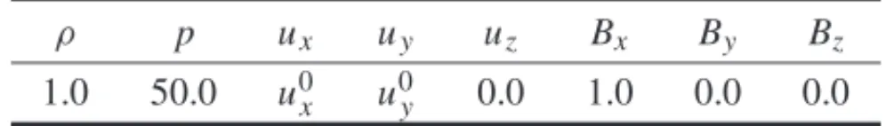
In fluids or plasmas, the Kelvin-Helmholtz instability is triggered by a velocity shear and cre-ates a vortex as discussed in [6]. That occurs in several phenomena in nature and space, in the clouds and magnetosphere, for instance [5]. In our simulations, we consider the initial conditions presented in Table 1, with
u0x =5(tanh(20(y+0.5))−(tanh(20(y−0.5))+1)),
u0y=0.25 sin(2πx)(exp[−100(y+0.5)2] −exp[−100(y−0.5)2]),
and periodic boundary conditions everywhere. The computational domain is = [0,1.0] × [−1.0,1.0] and the finest scale is L = 9. We also define as parameters the Courant number
ν = 0.4, γ = 1.4, and the physical timet = 0.5. The choice of resistivityη =0.02 is made according to astrophysics uses, as discussed in [5] and for the ideal case we considerη = 0. We have also tested other values ofη as [0.005,0.05]. We consider the threshold parameters
ǫ0 =0.1 and 0.01 both for the ideal and resistive cases. For the divergence-cleaning, we adopt
α=0.4, as discussed in [9].
Table 1: Kelvin-Helmholtz instability initial condition.
ρ p ux uy uz Bx By Bz
1.0 50.0 u0x u0y 0.0 1.0 0.0 0.0
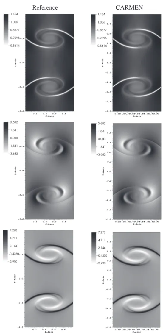
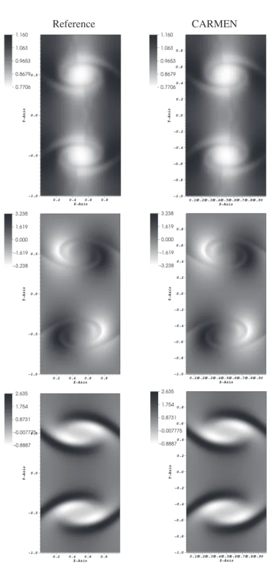
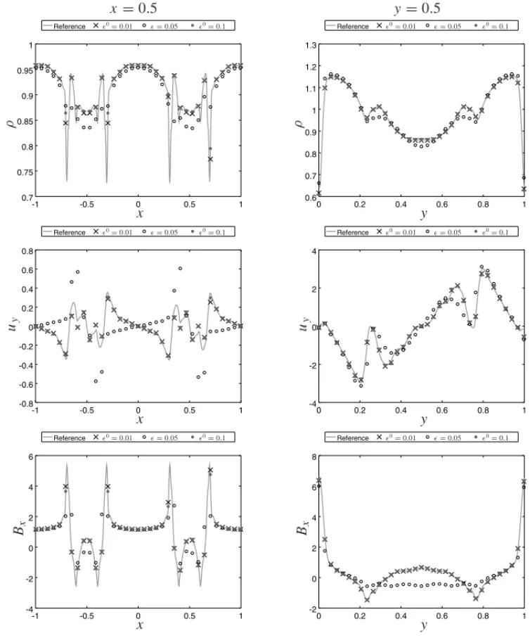
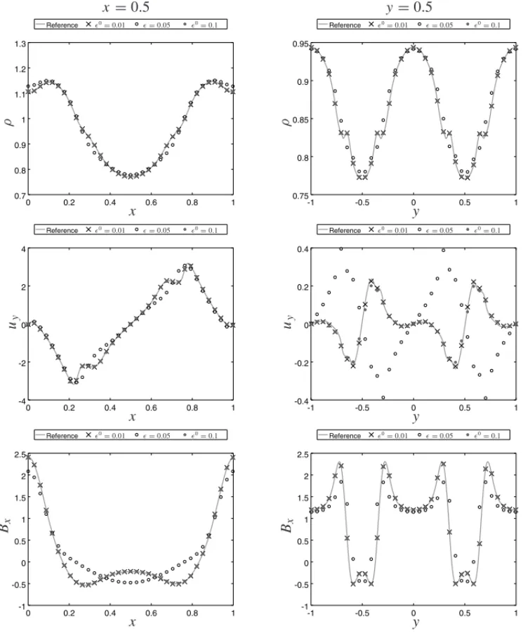
The reference (left) and CARMEN (right) code solutions for ideal and resistive MHD are pre-sented for the variables densityρ, velocityy-componentuy, and magnetic field x-component Bx in Figures 1 and 2. In both simulations the obtained results have the same maximum and minimum values. The larger gradients values in the solution are presented where the vortexes are located, near toy= −0.5 andy=0.5. For the variable density, for instance, it is possible to find gradients of one order of magnitude for the ideal case, and even not using the entire simulation mesh these structures are well captured. The resistive results are clearly more diffusive when compared to the ideal case, as expected, since it is the effect of the additional resistive terms. Figures 3 and 4 present the cuts for the variablesρ,uy, and Bx, in x = 0.5 and y = 0.5 at t =0.5, respectively, of reference and CARMEN code solutions for ideal and resistive MHD. These cuts are located where the most critical structures in solution are placed, due to many discontinuities, and they remain very close for each case with both codes.
Reference CARMEN
Reference CARMEN
the solution is not sufficient, which means that the number of cells used to represent the solution is not enough, thus it is important to find an acceptable threshold parameter in order to obtain a fair relation between CPU time, number of cells, and accuracy.
x =0.5 y=0.5
-1 -0.5 0 0.5 1 0.7 0.75 0.8 0.85 0.9 0.95 1 Reference ρ x
ǫ0=0.01 ǫ=0.05 ǫ0=0.1
0 0.2 0.4 0.6 0.8 1 0.6 0.7 0.8 0.9 1 1.1 1.2 1.3 Reference ρ y
ǫ0=0.01 ǫ=0.05 ǫ0=0.1
-1 -0.5 0 0.5 1 -0.8 -0.6 -0.4 -0.2 0 0.2 0.4 0.6 0.8 Reference uy x
ǫ0=0.01 ǫ=0.05 ǫ0=0.1
0 0.2 0.4 0.6 0.8 1 -4 -2 0 2 4 Reference uy y
ǫ0=0.01 ǫ=0.05 ǫ0=0.1
-1 -0.5 0 0.5 1 -4 -2 0 2 4 6 Reference Bx x
ǫ0=0.01 ǫ=0.05 ǫ0=0.1
0 0.2 0.4 0.6 0.8 1 -2 0 2 4 6 8 Reference Bx y
ǫ0=0.01 ǫ=0.05 ǫ0=0.1
To illustrate this situation, we can observe the cuts forǫ =0.05, which do not converge prop-erly to the reference solution when compared to the other two cases. However, this behavior is expected since the percentage of cells needed for those simulations are 11% and 5% for the ideal and resistive cases, respectively. This reinforces the importance of the choice of parameterǫ.
x=0.5 y=0.5
0 0.2 0.4 0.6 0.8 1 0.7 0.8 0.9 1 1.1 1.2 1.3 Reference ρ x
ǫ0=0.01 ǫ=0.05 ǫ0=0.1
-1 -0.5 0 0.5 1 0.75 0.8 0.85 0.9 0.95 Reference ρ y
ǫ0=0.01 ǫ=0.05 ǫ0=0.1
0 0.2 0.4 0.6 0.8 1 -4 -2 0 2 4 Reference uy x
ǫ0=0.01 ǫ=0.05 ǫ0=0.1
-1 -0.5 0 0.5 1 -0.4 -0.2 0 0.2 0.4 Reference uy y
ǫ0=0.01 ǫ=0.05 ǫ0=0.1
0 0.2 0.4 0.6 0.8 1 -1 -0.5 0 0.5 1 1.5 2 2.5 Reference Bx x
ǫ0=0.01 ǫ=0.05 ǫ0=0.1
-1 -0.5 0 0.5 1 -1 -0.5 0 0.5 1 1.5 2 2.5 Reference Bx y
ǫ0=0.01 ǫ=0.05 ǫ0=0.1
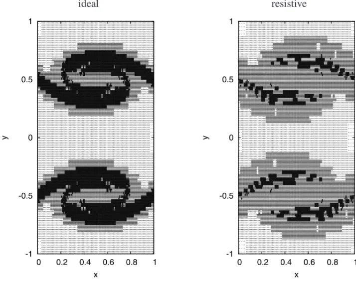
The adaptive meshes for the ideal and resistive cases at timet =0.5 are presented forǫ0 =0.1 in Figure 5. In this simulation the use of memory (percentage of cells) over time is 32% for the ideal case and 24% for the resistive case, when compared to a uniform mesh. The percentages of CPU time needed are 67% and 72% smaller for the ideal and resistive MHD, respectively. To quantitatively compare the presented results, Table 2 and 3 show theL1,L2, andL∞error values
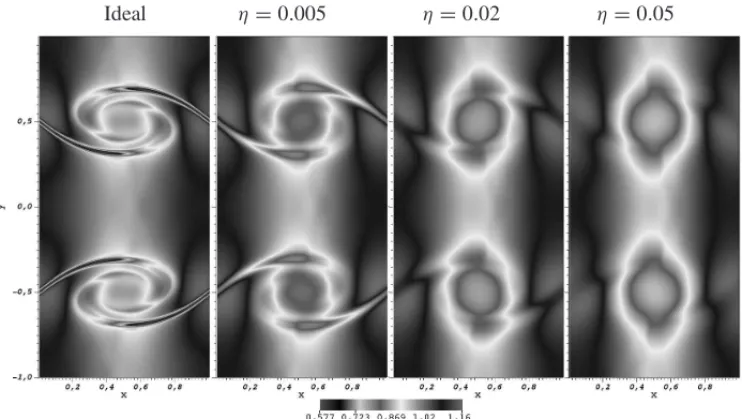
for every variable of the MHD model when the solution is compared with the reference results. The errors are computed for MR and FV CARMEN solutions and the reference solution. The values for the FV approach are slighty smaller when compared to the MR results. This result is expected since we need a full mesh in order to obtain them. The errors for the resistive case are even smaller when compared to the ideal case. That happens due to the diffusive behavior of the solution, since the greater values occur where the sharpest structures are located. In Figure 6, the diffusive behavior of the resistive terms of the MHD model is illustrated. We can observe how the topology of the solution of the variableρchanges according to the value ofη. In this case we chooseη=0 (ideal case),η=0.005,η=0.02 andη=0.05, and it shows that the solution becomes more diffusive asηis increased. As long as the local structures become more diffuse, the adaptive mesh for greater values ofηwill have less cells in the most refined level.
ideal resistive
-1 -0.5 0 0.5 1
0 0.2 0.4 0.6 0.8 1
y
x
-1 -0.5 0 0.5 1
0 0.2 0.4 0.6 0.8 1
y
x
Figure 5: Adaptive MR meshes att =0.5 obtained with CARMEN code withǫ0 =0.1 for the ideal and resistive cases.
Ideal η=0.005 η=0.02 η=0.05
Figure 6: Variable ρ obtained with CARMEN code at t = 0.5 for the ideal case and
η=0.005, η=0.02, η=0.05 (from left to right) andǫ0=0.1.
Table 2: Errors for the ideal Kelvin-Helmholtz simulation with MR (ǫ0=0.1) and FV compared with referece results.
CARMEN
Variables Errors
code L1(×10−2) L2(×10−4) L∞(×10−1)
FV
ρ 0.29 0.14 0.89
p 18.25 10.53 67.87
ux 6.57 4.32 22.86
uy 3.34 1.74 8.38
Bx 4.04 2.09 10.69
By 1.65 0.76 3.22
MR
ρ 0.30 0.14 1.00
p 18.38 9.10 60.11
ux 6.72 4.14 21.98
uy 3.82 1.83 8.43
Bx 4.08 1.81 8.63
By 1.91 0.80 3.37
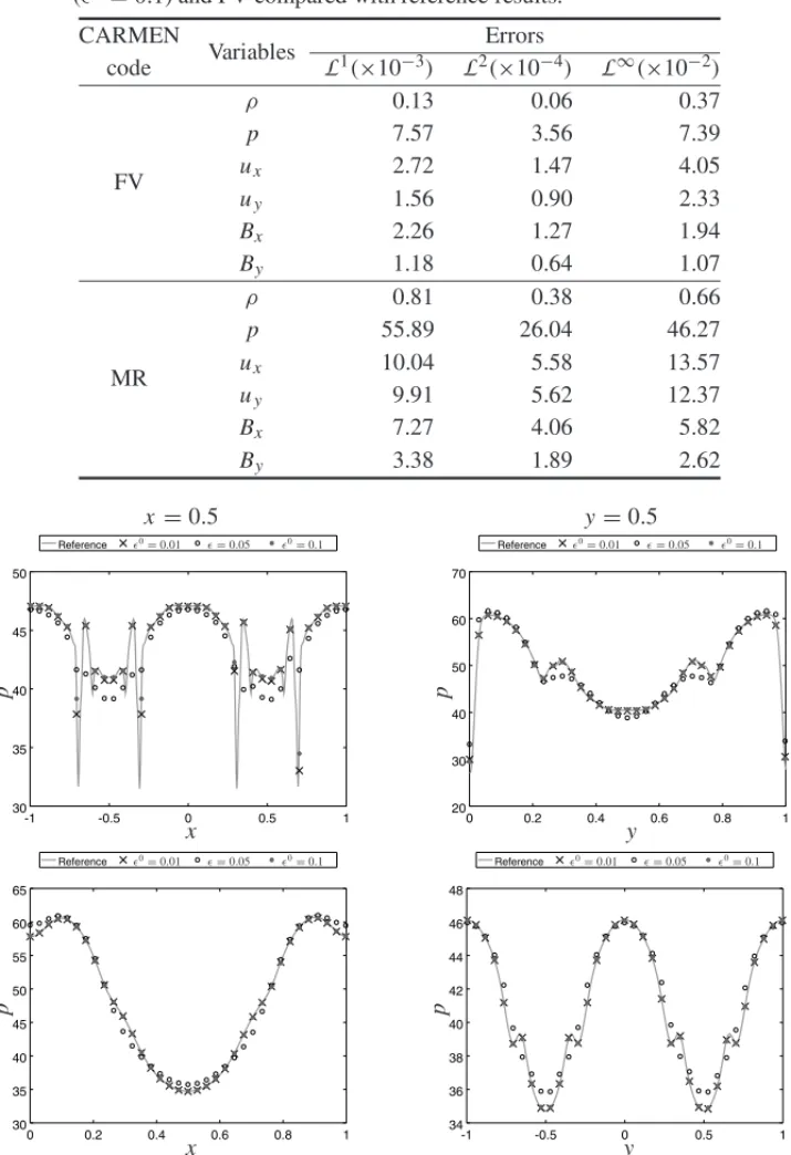
approximation errors of these variables accumulate in the pressure. In Figure 7 we observe that the solution of pis close to the reference solution on ideal (top) and resistive cases (bottom), for
Table 3: Errors for the resistive Kelvin-Helmholtz simulation with MR (ǫ0=0.1) and FV compared with reference results.
CARMEN
Variables Errors
code L1(×10−3) L2(×10−4) L∞(×10−2)
FV
ρ 0.13 0.06 0.37
p 7.57 3.56 7.39
ux 2.72 1.47 4.05
uy 1.56 0.90 2.33
Bx 2.26 1.27 1.94
By 1.18 0.64 1.07
MR
ρ 0.81 0.38 0.66
p 55.89 26.04 46.27
ux 10.04 5.58 13.57
uy 9.91 5.62 12.37
Bx 7.27 4.06 5.82
By 3.38 1.89 2.62
x=0.5 y=0.5
-1 -0.5 0 0.5 1 30 35 40 45 50 Reference p x
ǫ0=0.01 ǫ=0.05 ǫ0=0.1
0 0.2 0.4 0.6 0.8 1 20 30 40 50 60 70 Reference p y
ǫ0=0.01 ǫ=0.05 ǫ0=0.1
0 0.2 0.4 0.6 0.8 1 30 35 40 45 50 55 60 65 Reference p x
ǫ0=0.01 ǫ=0.05 ǫ0=0.1
-1 -0.5 0 0.5 1 34 36 38 40 42 44 46 48 Reference p y
ǫ0=0.01 ǫ=0.05 ǫ0=0.1
5 FINAL REMARKS
We have presented a wavelet based multiresolution approach to compute the Kelvin-Helmholtz instabilities for the ideal and resistive MHD system with parabolic-hyperbolic divergence clean-ing approach and compared its results to a reference solution obtained with FLASH code. New implementations of the resistive MHD model are done in CARMEN code for the MR and FV approaches. It is shown that the topology of the solution of the problem achieved with the adap-tive MR is very close to the reference solution and with the respecadap-tive cuts in the domain and the error values we ensure that it leads to the expected solution quantitatively. The adaptive method has proven to be efficient to keep the accuracy of the solution even decreasing the number of cells in the simulation. In our case we needed an average of 30% of cells for the simulations, which implied in a reduction of 67% of the CPU time (compared to the FV CARMEN code). We conclude that the presented MR methodology for the ideal and resistive MHD models is rel-evant in this instability context and it would be interesting to extend it to more complex space physics problems in future works.
ACKNOWLEDGEMENTS
M.O.D. and O.M. thankfully acknowledge financial support from MCTI/FINEP/INFRINPE-1 (grant 01.12.0527.00), CNPq (grants 30603-8/2015-3, 31224-6/2013-7) and FAPESP (grants 2015/50403-0, 2015/25624-2, 2016/50016-9). A.G. thankfully acknowledges financial support of MCTI/INPE-PCI and PhD scholarships from CNPq (grants 132045/2010-9, 312479/2012-3, 141741/2013-9). The software used in this work was in part developed by the DOE NNSA-ASC OASCR Flash Center at the University of Chicago. We thank Dr. Olivier Roussel for developing the original MR CARMEN code for hydrodynamics and Dr. Kai Schneider fruitful for scientific discussions. We also want to thank to Dr. Edgard Evangelista for his help with FLASH code and Eng. Varlei Menconi for the computational assistance.
RESUMO.Este trabalho refere-se `a simulac¸˜ao num´erica da instabilidade de
Kelvin-Helm-holtz usando um modelo magneto-hidrodinˆamico ideal e resistivo bidimensional no contexto de uma abordagem de multirresoluc¸ ˜ao adaptativa. As instabilidades de Kelvin-Helmholtz s˜ao
causada por uma velocidade de cisalhamento, e normalmente ´e esperada em uma camada
entre dois fluidos com diferentes velocidades. Devido `a sua complexidade, esse tipo de pro-blema ´e um teste bem conhecido para esquemas num´ericos, sendo importante para a
verifica-c¸˜ao do c ´odigo desenvolvido. O objetivo principal deste trabalho ´e verificar a implementaverifica-c¸˜ao
num´erica do modelo utilizando o conhecido c ´odigo FLASH, aplicado ao contexto das insta-bilidades de Kelvin-Helmholtz.
Palavras-chave:magneto-hidrodinˆamica, instabilidade de Kelvin-Helmholtz, an´alise
REFERENCES
[1] A. Dedner, F. Kemm, D. Kr¨oner, C.-D. Munz, T. Schnitzer & M. Wesenberg. Hyperbolic divergence cleaning for the MHD equations.Journal of Computational Physics,175(2002), 645–673.
[2] M.O. Domingues, S.M. Gomes, O. Roussel & K. Schneider. Adaptive multiresolution methods. ESAIM Proceedings,34(2011), 1–96.
[3] M.O. Domingues, A.K.F. Gomes, S.M. Gomes, O. Mendes, B. Di Pierro & K. Schneider. Extended generalized lagrangian multipliers for magnetohydrodynamics using adaptive multiresolution meth-ods.ESAIM Proceedings,43(2013), 95–107.
[4] R. Deiterding, M.O. Domingues, S.M. Gomes & K. Schneider. Comparison of adaptive multiresolu-tion and adaptive mesh refinement applied to simulamultiresolu-tions of the compressible euler equamultiresolu-tions.SIAM Journal on Scientific Computing,38(2016), S173–S193.
[5] E.F.D. Evangelista, M.O. Domingues, O. Mendes & O.D. Miranda. A brief study of instabilities in the context of space magnetohydrodynamic simulations.Revista Brasileira de Ensino de F´ısica,
38(1) (2016).
[6] A. Frank, T.W. Jones, D. Ryu & J.B. Gaalaas. The magnetohydrodynamic Kelvin-Helmholtz insta-bility: A two-dimensional numerical study.The Astrophysical Journal,460(1996), 777.
[7] B. Fryxell, K. Olson, P. Ricker, F.X. Timmes, M. Zingale, D.Q. Lamb, P. MacNeice, R. Rosner, J.W. Truran & H. Tufo. FLASH: An adaptive mesh hydrodynamics code for modeling astrophysical thermonuclear flashes.The Astrophysical Journal Supplement Series,131(2000), 273–334.
[8] A.K.F. Gomes. An´alise multirresoluc¸ ˜ao adaptativa no contexto da resoluc¸˜ao num´erica de um modelo de magnetohidrodinˆamica ideal. Master’s thesis, Instituto Nacional de Pesquisas Espaciais (INPE), S˜ao Jos´e dos Campos, (2012).
[9] A.K F. Gomes, M.O. Domingues, K. Schneider, O. Mendes & R. Deiterding. An adaptive multireso-lution method for ideal magnetohydrodynamics using divergence cleaning with parabolic–hyperbolic correction.Applied Numerical Mathematics,95(2015), 199–213.
[10] A. Harten. Multiresolution representation of data: a general framework.SIAM Journal of Numerical Analysis,33(3) (1996), 385–394.
[11] R.J. Hosking & R.L. Dewar. “Fundamental Fluid Mechanics and Magnetohydrodynamics”. Springer Singapore, (2016).
[12] T. Miyoshi & K. Kusano. A multi-state HLL approximate Riemann solver for ideal magnetohydro-dynamics.Journal of Computational Physics,208(2005), 315–344.
[13] A. Mignone & P. Tzeferacos. A second-order unsplit Godunov scheme for cell-centered MHD: The CTU-GLM scheme.Journal of Computational Physics,229(6) (2010), 2117–2138.
[14] K.G. Powell, P.L. Roe, T.J. Linde, T.I. Gombosi & D.L. De Zeeuw. A Solution-Adaptative Upwind Scheme for Ideal Magnetohydrodynamics.Journal of Computational Physics,154(1999), 284–309.
[15] O. Roussel, K. Schneider, A. Tsigulin & H. Bockhorn. A conservative fully adaptive multiresolution algorithm for parabolic{PDEs}.Journal of Computational Physics,188(2) (2003), 493–523.
[16] E.F. Toro. “Riemann Solvers and Numerical Methods for Fluid Dynamics: A Practical Introduction”.