Journal homepage:www.ijaamm.com
International Journal of Advances in Applied Mathematics and Mechanics
The effect of external source of disease on the epidemic model
Research Article
Ahmed Ali Mohsena,∗ Hanan Kasimb
aMinistry of Education, First Rusafa, Baghdad, Iraq
bDepartment of Mathematics, Baghdad University, College of Education Ibn al-Haytham of Pure Sciences, Baghdad, Iraq
Received 03 April 2015; accepted (in revised version) 28 May 2015
Abstract: In this paper a mathematical model that describes the flow of infectious disease in a population is proposed and stud-ied. It is assumed that the disease divided the population into three classes: susceptible individualsS, first infected individualsI and second infected individualsI∗. The main objective of this paper is to study the effect of external Source and treatment of behaviors of this model. The existence, uniqueness and boundedness of the solution of this model are investigated. The local and global dynamical behaviors of the model are studied. Finally, in order to confirm our obtained results and specify the effects of model’s parameters on the dynamical behavior, numerical simulation of this model is performed.
MSC: 92B05• 92B99
Keywords:Epidemic models •Stability •Treatment • External Source
© 2015 The Author(s). This is an open access article under the CC BY-NC-ND license(https://creativecommons.org/licenses/by-nc-nd/3.0/).
1. Introduction
The mathematical models have become important tools in analyzing the spread and control of infectious dis-eases. The development of such models is aimed at both understand observed epidemiological patterns and pre-dicting the consequences of the introduction of public health interventions to control the spread of diseases. Some diseases not confer immunity against the disease but other diseases confer immunity so recovered individuals gain immunity against disease. These types of disease can be modifications by SI and SIS where S susceptible and I infective respectively. Both epidemic models (SI and SIS) are one of the most basic and most important models in describing of many diseases. Therefore, it attached many authors attention and a number of papers have been published. For exam-ple Gao and Hethcote [1], considered an SIS model with a standard disease incidence and density-dependent demo-graphics. Li and Ma [2], studied an SIS model with vaccination and temporary immunity. Kermack and Mckendeick [3], proposed a simple SIS model with infective immigrants. X. Zhou [4], studied HBV infection disease. Muhammad A. [5], proposedSE I Repidemic model with non-linear saturated incidence and temporary immunity. In recent years, many papers found treatment function for example, Li et al [6] and Goodluck [7], proposed the SIS model with a lim-ited resource for treatment. Shurowq k. Shafeeq [8], studied the effect of treatment, immigrants and vaccinated on the dynamic of SIS epidemic model. In this paper we proposed and studied a mathematical model consisting of epidemic model with treatment, in which it is assumed that the disease transmitted by contact as well as external sources in the environment. The local as well as global stability analysis of this model is investigated.
∗ Corresponding author.
2. Model development
From a simple epidemiological model in which the total population ( say N(t)) at time t is divided into two sub classes the susceptible individuals S(t) and infected individualsI(t). Such model can be represented as follows:
d S
d t =Λ−β1SI−µS d I
d t =β1SI−µI
(1)
HereΛ>0 is the recruitment rate of the population,µ>0 is the natural death rate of the population,β1>0 is the
infected rate (incidence rate) of susceptible individuals due to directed contact with the infected individuals. Now, since there are many infectious disease for example (The flue., tube rculosis and cholera), spread in the environment by different factors including insects, contact or other vectors, therefore, we assumed that the disease in the a above model will transmitted between the population individuals by contact as well as external source of disease in the envi-ronment with an external source incidence rateβ◦≥0 . Also it is assumed that the nature recovery rate from infected individuals returns to be susceptible class with a constant rateα≥0 andψ≥0 is the rate of infected individuals from disease I into new diseaseI∗. Finallyθ>0,β2>0 the disease related death from second disease and the infected
rate by contact between the susceptible individuals and infected individuals of second disease respectively. Then if addition above assumption system (1) can be rewritten in the form:
d S
d t =Λ−(β◦+β1I+β2I
∗)S−µS+αI
d I
d t =(β◦+β1I)S−(α+µ+ψ)I d I∗
d t =β2SI
∗+ψI−(µ+θ)I∗
(2)
Keeping the above in view, in order to study the effect of treatment on the system (2) letT(I) represented the treatment function which given by [6]:
T(I)= (
r I∗ i f 0<I∗ÉI◦∗,
k i f I∗>I◦∗. (3)
Therefore, system (2) can be modified to:
d S
d t =Λ−(β◦+β1I+β2I
∗)S−µS+αI+T(I∗)
d I
d t =(β◦+β1I)S−(α+µ+ψ)I d I∗
d t =β2SI
∗+ψI−(µ+θ)I∗−T(I∗)
(4)
herk=r I◦∗this means that the treatment rate is proportional to the number of the infected individuals when the capacity of treatment is not reached, and otherwise takes the maximal capacity. Therefore at any point of time t the total number of population becomesN(t)=S(t)+I(t)+I∗(t). Obviously, due to the biological meaning of the variables
S(t),I(t) andI∗, system (4) has the domainR3+=©
(S,I,I∗)∈R3+,S≥0,I≥0,I∗≥0ª
which is positively in variant for system (4). Clearly, the interaction functions on the right hand said of system (4) are continuously differentiable. In fact they are Liptschizan function onR3+. Therefore, the solution of system (4) exits and unique. Further, all solutions of system (4) with non-negative initial conditions are uniformly bounded as shown in the following theorem.
Theorem 2.1.
All the solutions of system(1), which are initiate in R+3, are uniformly bounded.
Proof. Let¡
S(t),I(t),I∗(t)¢
be any solution of the system (4) with non-negative initial conditions¡
S(0),I(0),I∗(0)¢ . SinceN=S(t)+I(t)+I∗(t), then:
d N d t =
d S d t +
d I d t +
d I∗ d t
This gives:
d N
d t =Λ−µ ©¡
So,
d N
d t +µNÉΛ
Now, by using Gronwall Lemma [?], it obtains that:
N(t)≤Λ µ(1−e
−µt
)+N(0)e−µt
Therefore,N(t)≤Λ
µ,as→ ∞, hence all the solutions of system (4) that initiate inR 3
+are confined in the reign:
Γ= ½
(S,I,I∗)∈R+3:N≤Λ µ ¾
which complete the proof.
3. Existence of equilibrium point of system
(
4
)
The system (4) has at most three biologically feasible points, namelyEi =(Si,Ii,Ii∗),i =0, 1, 2. The existence conditions for each of these equilibrium points are discussed in the following:
1) If I =0 andI∗=0, then the system ((??) has an equilibrium point called a disease free equilibrium point and denoted byE0=(S0, 0, 0) where:
S0=Λ
µ (5)
2) IfI∗=0, then the system (4) has an equilibrium point called a second disease free equilibrium point and denoted byE1=(S1,I1, 0) whereS1andI1represented the positive solution of the following set of equations:
Λ−(β◦+β1I)S−µS+αI=0
(β◦+β1I)S−(α+µ)I=0 (6)
From Eq. (1) of above system we get:
S1= Λ+αI1
β◦+β◦I1+µ (7)
SubstitutingS1in Eq. (2) of system (6) we get:
I1=−D2 2D1−
1 2D1
q
D22−4D1D3 (8)
here
D1= −β1µ D2=Λ
©
β1−µ(β◦+α+µ) ª
D3=β◦Λ
Clearly, Eq. (8) has a unique positive root byI1and then (E2) exists uniquely in Int.R+3if and only ifD2>0.
3)If I6=0 andI∗6=0 then the system (4) has an equilibrium point called endemic equilibrium point and denoted byE2=(S2,I2,I2∗), where,S2,I2and I2∗represented the positive solution of the following set of equations in case
(0<I∗<I◦∗) of Eq. (3) (treatment function):
Λ−(β◦+β1I+β2I∗)S−µS+αI+r(I∗)=0 (β◦+β1I)S−(α+µ+ψ)I=0
β2SI∗+ψI−(µ+θ−r)I∗=0
(9)
Straightforward computation to solve the above system of equations and from Eqs. (2) and3of system (9) gives that:
S2=(µ+α+ψ)I2 β2+β1I2
I2∗=
−ψI2(β◦+β1I2
β2I2(µ+α+ψ)−(µ+θ+r)(β◦+β1I2) (11)
While,I2∗positive root if and only if
β2I2(µ+α+ψ)<(µ+θ+r)(β◦+β1I2)
Now, substitutingS2andI2∗in Eq. (1) of system (9) we get:
A1I23+A2I22+A3I2+A4=0 (12)
here
A1=β1 ©
(µ+α+ψ)£
β1(µ+θ+r)+αβ2 ¤
+β1ψr−[β2(µ+α+ψ)2+β2ψ(µ+α+ψ)+β1α(µ+θ+r)] ª
A2=©2β◦β1ψr+(µ+α+ψ) £
Λβ1β2+β◦β2α+β◦β1(µ+θ+r) ¤
− £
β2(µ+α+ψ) £
β◦ψ+(β◦+µ)(µ+α+ψ)¤
+β1(µ+θ+r) (Λβ1+2αβ◦) ¤ª
A3=©(µ+α+ψ)£
Λβ◦β2+(µ+θ+r) ¡
β2◦+β◦β1+β◦µ+β1µ ¢¤
+β2◦ψr−β◦(µ+θ+r)(2β1+αβ◦) ª
A4= −Λβ2◦(µ+θ+r)<0
A4= −Λβ2◦(µ+θ+r)<0
Clearly, Eq. (12) has a unique positive root byI2and then (E2) exists uniquely in IntR+3. if and only ifA1>0 then we have the following three cases:
Case (1):If the following conditions hold:
A2>0
A3>0 (13)
Case (2):If the following conditions hold:
A2<0
A3<0 (14)
Case (3):If the following conditions hold:
A2>0
A3<0 (15)
4. Local Stability of system
(
4
)
In this section, the local stability analysis of the equilibrium pointsEi,i =0, 1, 2 of the system (4) studied as shown in the following theorems.
Theorem 4.1.
The disease free equilibrium point E◦=(Λ
µ, 0, 0)of system(4)is locally asymptotically stable provided that:
α<β1Λ
µ <µ+α+ψ (16)
r<β2Λ
µ <µ+θ+r (17)
µ β1Λ
µ −α ¶ ·
β◦+2µ+α+ψ−β1Λ µ
¸
>ψ(r−β2Λ
Proof. The Jacobian matrix of system (4) atE◦that denoted byJ(E◦) and can be written as
J(E◦)=£ ai j¤3×3
where
a11= −(β◦+µ);a12=α−β1Λ
η ;a13=r− β2Λ
µ
a21=β◦;a22=β1Λ
µ −(µ+α+ψ);a23=a31=0
a32=ψ;a33=β2Λ
µ −(µ+θ+r)
Then the characteristic equation ofJ(E◦) is given by:
λ3+Ω1λ2+Ω2λ+Ω3=0 (19)
here
Ω1= −[a11+a22+a33]=(β◦+µ)− ¡
β1S0−(µ+α+ψ)¢
−¡β2S0−(µ+θ+r)¢ Ω2=a11a22−a12a21+a11a33+a22a33
Ω3=[a12a21a33−a11a22a33−a21a32a13] =£β◦¡
α−β1S0¢ ¡
β2S0−(µ+θ+r)¢
+¡β◦+µ¢ ¡
β1S0−(µ+α+ψ)¢ ¡
β2S0−(µ+θ+r)¢
−β◦ψ(r−β2S0)¤
Further
∆=Ω1Ω2−Ω3= −a211(a22+a33)−a 2
22(a11+a33)−a 2
33(a11+a22)−a11a22a33+a21[a12(a11+a22)+a32a13]
= −¡β◦+µ¢2£
β1S0−(µ+α+ψ)+β2S◦−(µ+θ+r)¤
−¡β1S0−(µ+α+ψ)¢2£
−(β◦+µ)+β2S◦−(µ+θ+r)¤
−¡β2S◦−(µ+θ+r)¢2£
−(β◦+µ)+β1S0−(µ+α+ψ)¤
+(β◦+µ)(β1S0−(µ+α+ψ)(β2S◦−(µ+θ+r)+β◦× £
(α−β1S0)¡
−(β◦+µ)+β1S0−(µ+α+ψ)¢
+ψ(r−β2S0¤
Now, according to (Routh-Hurwitz) criterion [10],E0will be locally asymptotically stable provided thatΩ1>0 and Ω3>0. Clearly, provided that conditions (16)-(17) hold. While,∆=Ω1Ω2−Ω3>0 Provided that conditions (16)-(18)
hold. Hence the proof is complete.
Theorem 4.2.
The second disease free equilibrium point(E1)of system(4)is locally asymptotically stable if the following sufficient conditions are satisfied:
µ>M ax.©
2(β1S1−α−ψ), 2(β2S1−r)−θª
(20)
Proof. The Jacobian matrix of system (4) at (E1) that denoted byJ(E1) can be written as:
J(E1)=£ bi j
¤ 3×3
Where
b11= −(β◦+β1I1+µ) ; b12=α−β1S1; b13=r−β2S1 b21=β◦+β1I1;b22=β1S1−(µ+α+ψ) ;b23=0 b31=0 ; b23=ψ;b33=β2S1−(µ+θ+r)
Now, according to Gersgorin theorem [11] if the following condition holds:
|bi i| >
3 X
i=1,i6=j ¯ ¯bi j
¯ ¯
Then all eigenvalues ofJ(E1) exists in the region:
℘= ∪ (
U∗∈C:¯ ¯U∗−bi i
¯ ¯<
3 X
i=1,i6=j ¯ ¯bi j
¯ ¯ )
Therefore, according to the given condition (20) all the eigenvalues ofJ(E1) exists in the left half plane and hence,E1
Theorem 4.3.
The endemic equilibrium point(E2)of system(4)is locally asymptotically stable if the following sufficient conditions are satisfied:
µ>M ax.©2(β1S2−α−ψ), 2(β2S2−r)−θª (21)
Proof. The Jacobian matrix of system (4) at (E2) that denoted byJ(E2) can be written as:
J(E2)=£ ci j
¤ 3×3
Where:
c11= −(β◦+β1I2+β2I2∗+µ) ; c12=α−β1S2; c13=r−β2S2 c21=β◦+β1I2; c22=β1S2−(µ+α+ψ) ; c23=0
c31=β2I2∗;c23=ψ;c33=β2S2−(µ+θ+r)
Now, according to Gersgorin theorem [8] if the following condition holds:
|ci i| >
3 X
i=1,i6=j ¯ ¯ci j
¯ ¯
Then all eigenvalues ofJ(E2) exists in the region:
ς= ∪ (
U∗∈C:¯¯U∗−ci i ¯ ¯<
3 X
i=1,i6=j ¯ ¯ci j
¯ ¯ )
Therefore, according to the given condition (21) all the eigenvalues ofJ(E2) exists in the left half plane and hence,E2
is locally asymptotically stable.
5. Globally stability of all equilibrium point
In this section, the global dynamics of system (4) is studied with the help of Lyapunov function as shown in the following theorems.
Theorem 5.1.
Assume that, the disease free equilibrium point E0of system(4)is locally asymptotically stable. Then the basin of attrac-tion of E0, say B(E0)⊂R+3, it is globally asymptotically stable if satisfy the following condition:
¡
β◦+β1I+β2I∗S¢<¡αI+r I∗¢ (22)
Proof. Consider the following positive definite function:
V1= µ
S−S0−S0l n S S0
¶ +I+I∗
Clearly,V1:R+3→Ris a continuously differentiable function such thatV1(S0, 0, 0)=0 andV1(S,I,I∗)>0,∀(S,I,I∗)6= (S0, 0, 0). Further we have:
dV1 d t =
µ S−S0
S 
d S d t +
d I d t +
d I∗ d t
By simplifying this equation we get:
dV1 d t = −
µ S(S−S0)
2 +
·
β◦+β1I+β2I∗−(αI+r I ∗)
S ¸
S0−µ(I+I∗)−θI∗
Obviously,dV1
Theorem 5.2.
Assume that, the second disease free equilibrium point E1of system(4)is locally asymptotically stable. Then the basin of attraction of E1, say B(E1)⊂R+3, it is globally asymptotically stable if satisfy the following conditions:
µ
β1S1I−(αI+β◦S+β1SI1 SI
¶2 <4
µ
µ+α+ψ−β1S I
¶ µ
β◦+µ+β1I S
(23)
¡ β2S1I∗¢
<¡r S1+(µ+θ)S¢
I∗ (24)
Proof. Consider the following positive definite function:
V2= µ
S−S1−S1l n S S1
¶ +
µ
I−I1−I1l n I I1
¶ +I∗
Clearly,V2:R+3→Ris a continuously differentiable function such thatV2(S1,I1, 0)=0 andV2(S,I,I∗)>0,∀(S,I,I∗)6= (S1,I1, 0). Further we have:
dV2 d t =
µ S−S1
S 
d S d t +
µ I−I1
I 
d I d t +
d I∗ d t
By simplifying this equation we get:
dV2
d t = −q11(S−S1) 2
−q12(S−S1)(I−I1)−q22(I−I1)2−(β2− r
S)(S−S1)I
∗+β2SI∗+ψI−(µ+θ+r)I∗
With:
q11=β◦+µ+β1I
S ;q22=
(µ+α+ψ)−β1S
I ;
q12=β1S1I−(αI+β◦S+β1SI1) SI
Therefore, according to (23) it is obtaining that:
dV2 d t É −
£p
q11(S−S1)+pq22(I−I1)¤2
+β2S1I∗+ψI−¡
r S1+(µ+θ)S¢ I∗
Obviously,dV2
d t <0 for every initial points satisfying condition (24) and thenV2is a Lyapunov function provided that
conditions (23)-(24)) hold. ThusE2is globally asymptotically stable in the interior ofB(E2), which means thatB(E2) is the basin of attraction and that complete the proof.
Theorem 5.3.
Let the endemic equilibrium point E2of system(4)is locally asymptotically stable. Then it is globally asymptotically stable provided that:
M ax. ½
µ+α+ψ β1
,µ+θ+r
β2 ¾
<S2 (25)
(β◦+β1I+α−β1S2)2<(β◦+µ+β1I+β2I∗)(µ+α+ψ−β1S2) (26)
(β2I∗+r−β2S2)2<(β◦+µ+β1I+β2I∗)(µ+θ+r−β2S2) (27)
Proof. Consider the following positive definite function:
V3=(S−S2) 2
2 +
(I−I2)2
2 +
(I∗−I2∗)2 2
Clearly,V3:R+3→Ris a continuously differentiable function such thatV3(S2,I2,I2∗)=0 andV3(S,I,I∗)>0,∀(S,I,I∗)6= (S2,I2,I2∗). Further we have:
dV3
d t =(S−S2) d S
d t +(I−I2) d I d t+(I
∗−I∗ 2)
d I∗ d t
By simplifying this equation we get:
dV3 d t = −
p11
2 (S−S2)
2
+p12(S−S2) (I−I2)−p22 2 (I−I2)
2 −p11
2 (S−S2)
2
+p13(S−S2)¡ I∗−I2∗¢
−p33 2
¡
I∗−I2∗¢2 −p22
2 (I−I2)
2
+p23(I−I2)¡ I∗−I2∗¢
−p33 2
¡
I∗−I2∗¢2
with
p11=¡β◦+µ+β1I+β2I∗¢
; p12=¡β◦+β1I+α−β1S2¢ p22=(µ+α+ψ)−β1S2; p13=¡β2I∗+r−β2S2¢ p33=(µ+θ+r)−β2S2; p23=ψ
Therefore, according to the conditions (25)-(28) we obtain that:
dV3 d t É −
·r p11
2 (S−S2)− r
p22
2 (I−I2) ¸2
− ·r
p11
2 (S−S2)+ r
p33
2 ¡
I∗−I2∗ ¢
¸2 −
·r p22
2 (I−I2)+ r
p33
2 ¡
I∗−I2∗ ¢
¸2
Obviously, dV3
d t <0, and thenV3is a Lyapunov function provided that conditions (25)-(28) hold. ThusE3is globally
asymptotically stable.
6. Numerical Simulation
In this section, the system (1) is solved numerically for different sets of hypothesis data and different sets of initial conditions, and then the time series for the trajectories of system (1) are confirm our obtained analytical results. By using (150, 100, 90), (250, 200, 150) and (350, 150, 200) as initial points and the numerical simulations are carried out in the following cases:
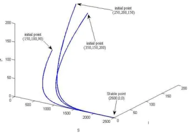
Case IFor the disease free equilibrium pointE0, we choose the following data:
Λ=500,β◦=0,β1=0.001,β2=0.001,µ=0.2,α=2,r=2,ψ=0.6,θ=0.4 (29)
Therefore, the disease free equilibrium pointE0of system (1) is globally asymptotically stable and then the trajectories of the system (1) is approaches to (2500,0,0) for any time. (SeeFig. 1)
Case IIFor the second equilibrium pointE1, we choose the following data and using (150, 100, 90), (250, 200, 150) and (350, 150, 200) as initial points:
Λ=500,β◦=0.1,β1=0.001,β2=0.001,µ=0.2,α=2,r=2,ψ=0,θ=0.4 (30)
Therefore, the second equilibrium pointE1of system (1) is globally asymptotically stable and then the trajectories of the system (1) is approaches to (1890,609,0) for any time. (SeeFig. 2)
Case IIIFor the endemic equilibrium pointE2, we choose the following data and using (150, 100, 90), (250, 200, 150) and (350, 150, 200) as initial points:
Λ=500,β◦=0.1,β1=0.001,β2=0.001,µ=0.2,α=2,r=2,ψ=0.6,θ=0.4 (31)
Therefore, the endemic equilibrium pointE2of system (1) is globally asymptotically stable and then the trajectories of the system (1) is approaches to (1845,193,153) for any time. (SeeFig. 3)
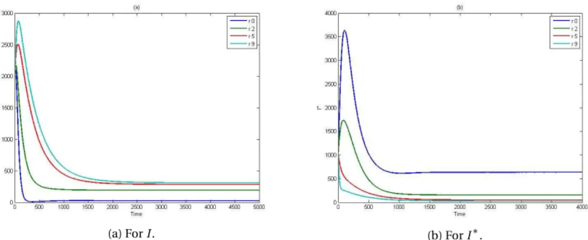
Case IVWe choose the incidence rate of disease resulting from external sourcesβ◦=0, 0.3, 0.6 respectively, keeping other parameters fixed as given in Eq. (31), we get the disease free equilibrium point of system (1) becomes unstable point and the trajectory of system (1) approaches asymptotically to the endemic equilibrium point. but the number of infected in first disease individuals and infected in second disease individuals increases. (SeeFigs. 4(a)-4(b)), Similar results are obtained, as those shown in case of increasingβ◦, in case of increasing the incidence rate of disease resulting by contact between susceptible and infected in first disease, that is means increasingβ1but increasing the
incidence rate of disease resulting by contact between susceptible and infected in second diseaseβ2and keeping
other parameters fixed as given in (31) we get the number of infected in first disease individuals decrease and infected in second disease individuals increase.
Fig. 1.Phase plot of system (1) starting from different initial points which show thatE0is globally asymptotically stable.
Fig. 2.Phase plot of system (1) starting from different initial points which show thatE1is globally asymptotically stable.
7. Conclusion and discussion
In this paper, we proposed and analyzed an epidemiological model that described the dynamical behavior of an epidemic model, where the infectious disease transmitted directly from external sources as well as through contact between them. The model included fore non-linear autonomous differential equations that describe the dynamics of three different populations namely susceptible individuals (S) infected individuals for first disease (I) and infected individuals for second disease (evolution of first disease) (I∗). The boundedness of system (1) has been discussed. The conditions for existence, stability for each equilibrium points are obtained. Further, it is observed that the disease free equilibrium pointE0exists whenI =0 and locally stable if the conditions are hold (16)-(18) and it is globally stable if and only if the condition (22) holds. The second disease free equilibrium pointE1exists if (D2>0) holds and locally stable if the conditions (20) are hold while it is globally stable if and only if the conditions (21)-(23)) hold. The endemic equilibrium pointE2exists if (A1>0) and one of three conditions is hold (13)-(15), and locally stable if the conditions (21) hold more than it is globally stable if and only if the conditions (25)-(28) hold. Finally, to understand the effect of varying each parameter on the global system (1) and confirm our above analytical results, the system (1) has been solved numerically for different sets of initial points and different sets of parameters given by Eq. (29), and the following observations are made:
Fig. 3.Phase plot of system (1) starting from different initial points which show thatE2is globally asymptotically stable.
(a) ForI. (b) ForI∗.
Fig. 4.Time series of the trajectories of system (1).
2. As the incidence rate of disease (external incidence rateβ◦orβ1contact incidence rate) increase, the asymptotic
behavior of the systems (1) approaching to endemic equilibrium point. In fact areβi,i = ◦, 1 increase it are observed that the number of (S) decrease and the number of (I) andI∗increase.
3. As the incidence rate of disease (contact incidence rateβ2) increase, the asymptotic behavior of the systems (1)
approaching to endemic equilibrium point. In fact asβ2increase it is observed that the number of (S) and (I)
(a) ForI. (b) ForI∗.
Fig. 5.Time series of the trajectories of system (4).
Acknowledgment
I would like to thank Dr. Raid K. Naji for to help me to finish this my paper
References
[1] L.Q. Gao, H.W. Hethcote, Disease models of with density-dependent demographics, J. Math. Biol. 50 (1995), 17– 31.
[2] J. Li, Z. Ma, Qualitative analysis of SIS epidemic model with vaccination and varying total population size, Math. Comput. Model 20(43) (2002) 12–35.
[3] W.O. Kermack, A.G. Mckendrick, Contributions to mathematical theoryof epidemics, Proc. R. Soc. Lond. A. 115 (1927) 700–721.
[4] Xueyong Zhou, Stability analysis of a fractional-order HBV infection model, Int. J. Adv. Appl. Math. and Mech. 2 (2014) 1–6.
[5] A. Kh. Muhammad , W. Abdul, Saeed I., Ilyas Kh., Sharidan Sh., Stability analysis of an SEIR epidemic model with non-linear saturated incidence and temporary immunity, Int. J. Adv. Appl. Math. and Mech. 3(2015) 1–14. [6] X.Z. Li. et. al., Stability and bifurcation of an SIS epidemic model with treatment, J. Chaos, Solution and Fractals,
42 (2009) 2822–2832.
[7] Goodluck, L. Livingstone, K. Dmitry, S. Francis, Optimal treatment and vaccination control strategies for the dynamics of pulmonary tuberculosis, Int. J. Adv. Appl. Math. and Mech. 3 (2015) 196-207.
[8] Shurowq k. Shafeeq, The effect of treatment, immigrants and vaccinated on the dynamic of SIS epidemic model. M.Sc. thesis. Department of Mathematics, College of Science, University of Baghdad. Baghdad, Iraq, 2011. [9] M. W. Hirsch, S. Smale, Differential Equation, Dynamical System, and Linear Algebra. Academic Press, Inc., New
York. (1974) 169-170.