Determination of the kinematic viscosity
by the liquid rise in a capillary tube
(Determina¸c˜ao da viscosidade cin´etica atrav´es da subida de um l´ıquido num tubo capilar)
J.L.G. Santander
1, G. Castellano
Departamento de Ciencais Experimentales y Matem´aticas, Universidad Cat´olica de Valencia, Valencia, Spain Recebido em 16/10/2012; Aceito em 14/3/2013; Publicado em 19/9/2013
We discuss first the valid time interval of a formula found in the literature which gives the theoretical dis-tance run by a liquid which rises along a capillary tube as a function of time. A non-linear least square fitting of experimental data to this theoretical curve allows the measurement of the kinematic viscosity of the liquid. The goodness of the fitting for three different sets of experimental data given in the literature is above 99%.
Keywords: viscosity, kinematic viscosity.
Discutimos inicialmente a validade do intervalo de tempo fornecido por uma f´ormula encontrada na literatura, que d´a a distˆancia percorrida em fun¸c˜ao do tempo para um l´ıquido que sobe num tubo capilar. Um ajuste n˜ao linear de m´ınimos quadrados dos dados experimentais com essa f´ormula permite a medida da viscosidade cin´etica do fluido. A qualidade do ajuste para dois conjuntos de dados experimentais daliteraura ´e acima de 99%. Palavras-chave: viscosidade, viscosidade cin´etica.
1. Introduction
The rise rate of a liquid in a capillary tube depends on its viscosity. However, the familiar laboratory exper-iments involving the rise of liquids in capillary tubes ignores this fact and the attention is focused on the sta-tionary regime. Despite it is described in the literature a very simple method for the experimental determina-tion of the kinematic viscosity using a capillary tube [1], this method does not take into account the effect of surface tension and does not give a statistical proce-dure for the determination of the experimental error. The falling sphere viscosimeter, based on the Stokes’ law, allows the determination of the kinematic viscos-ity from the measurement of the terminal velocviscos-ity of a sphere falling into a liquid [2, Eq. (4.9.20)], but we need to assure that the Reynolds number is small enough to apply the Stokes’ law and to know how much time is needed for the falling sphere to reach the stationary regime. Other classical experimental setups for the de-termination of the kinematic viscosity are principally based on the liquid motion into a capillary [3], or the friction that exerts a liquid over a rotating cylinder [4]. Nevertheless, all these classical methods assume implic-itly a stationary regime in the motion of the liquid, but there is a lack of discussion over this point.
In this work, we offer a method for the
experimen-tal determination of the kinematic viscosity of a liquid which is rising through a capillary tube, taking into ac-count the transient regime. In order to perform this measurement, firstly we discuss the valid time interval of the theoretical distance run by the liquid along the capillary as a function of time [5, 6] and its approxima-tion to the Lucas-Washburn equaapproxima-tion [7, 8]. Secondly, the theoretical curve for the liquid rise allows us to per-form a non-linear least square fitting to experimental data, so that we may determine the kinematic viscosity of the liquid. The goodness of the non-linear fitting for three different sets of experimental data given in the literature is above 99%.
2.
Time-dependent theoretical rise
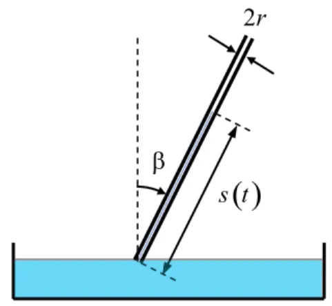
Let us consider a liquid of constant densityρ which is rising through a capillary tube of radiusr inclined an angle β with respect to the vertical, as shows Fig. 1. The forceF that the liquid experiments along the cap-illary is due to the surface tensionγ upwards, and the weight of the liquid downwards, so that
F= 2πrγcosθ−ρgπr2cosβ s(t), (1) 1E-mail: [email protected].
( )
s t
β
2
r
Figure 1 - Liquid rising through a capillary tube of radius r in-clined an angleβwith respect to the vertical.
where θ is the contact angle between the liquid and the capillary, ands(t) is the distance run by the liquid along the capillary as a function of timet.
Therefore, according to Eq. (1), there is a pressure difference which makes the liquid rise along the capil-lary
∆P = F
πr2 =
2γcosθ
r −ρgcosβ s(t). (2)
Poiseuille’s law [9, Eq. (17.10)] gives an expression for the volume discharge Qof a liquid of dynamic viscos-ity η flowing in laminar regime through a pipe of cir-cular cross section of radius r and length s, in which extrema we apply a pressure difference ∆P. Applying Poiseuille’s law, according to Eq. (2), we have
Q= πr 4∆P 8ηs =
πr3 4η
(γcosθ
s(t) −
ρgrcosβ
2
)
. (3)
Since most liquids in usual conditions are incompress-ible, the volume dischargeQis
Q=πr2 s′
(t). (4)
Equating Eq. (3) with Eq. (4), we have the following ODE,
s′
(t) = r 4η
(γcosθ
s(t) −
ρgrcosβ
2
)
. (5)
We may find Eq. (5) in Ref. [10] for a contact an in-clination angles both null, θ =β = 0. Assuming that the lower end of the capillary is initially just beneath the surface of the liquid, we have to take in Eq. (5) as initial condition,
s(0) = 0. (6)
In the stationary regime, the liquid does not rise any more, so that the distance covered by it is maximum,
s=smax, and the velocity of the liquid is null, s′ (t) = 0. Thus, according to Eq. (5), we have,
smax= 2γcosθ
ρgrcosβ. (7)
Equation (7) is known as Jurin’s law [11]. If we neglect the gravity term in Eq. (5), we have
γcosθ s(t) ≫
ρgrcosβ
2 ,
so, according to Eq. (7),
s(t)≪ ρgr2γcoscosθβ =smax, (8)
and Eq. (5) becomes
1 2
d dt
[
s2(t)]
=s(t)s′
(t)≈γr4cosη θ. (9)
Taking into account the initial condition (6) we may solve Eq. (9), arriving to
s(t)≈ √
γrcosθ
2η t, (10)
which is known as Lucas-Washburn equation [7,8]. No-tice that Eq. (10) is a good approximation when Eq. (8) is satisfied, that is, at the first stage of the liquid rise. Therefore, substituting Eq. (10) in Eq. (8), Lucas-Washburn equation is a good approximation when
t≪τ0:=
8ηγcosθ
ρ2g2r3cos2β. (11) In the literature [5,6], we may find the explicit solution of Eq. (5)
s(t) =smax
{
1 + W
[ −exp
(
−1−gr
2cosβ 8νsmax
t
)]}
,
(12) whereν is the kinematic viscosity,
ν:= η
ρ.
and the Lambert W function is the inverse function of
zez
[12]. Straightforward from the Lambert W function definition, we have W(
−e−1)
=−1 and W (0) = 0 [12], so Eq. (12) satisfies the initial condition (6)
s(0) =smax[1 + W(−e−1)]= 0, and the stationary regime (7)
lim
t→∞s(t) =smax [
1 + W(
−e−∞)]
=smax.
There is a very simple connection between Eq. (10) and Eq. (12) that, as far as we know, it is absent in the literature. If we define the functionα(t) as the height proportion reached at timet,
α(t) := s(t)
smax
and the parameter
κ:=gr 2cosβ
8νsmax , (14)
we may rewrite Eq. (12) as
α(t, κ) = 1 + W(
−e−1−κt)
. (15) Remembering the definition of the Lambert W function as the inverse function of zez
, we may invert Eq. (15) obtaining
t(α) =−1
κ[α+ log (1−α)]. (16)
In the first stage of the liquid rise, we have α≈0, so we may take the following approximation in Eq. (16) log (1−α)≈ −α−α2/2, thus,
t(α)≈α
2
2κ. (17)
Inverting in Eq. (17) and taking into account Eq. (13), we arrive to
s(t)≈smax
√
2κt, t&0. (18)
Substituting now Eq. (7) and Eq. (14) in Eq. (18), we recover the Lucas-Washburn equation (10).
In order to know the valid time range for Lucas-Washburn equation, notice that from Eq. (12) we can define the following characteristic time for the liquid rise,
t0:= 1
κ=
8νsmax
gr2cosβ =
16ηγcosθ
ρ2g2r3cos2β, (19) so, according to Eq. (12), the proportion of distance covered with respect to smax at the relaxation timet0 is
α(t0) = 1 + W( −e−2)
≈84.14%.
Therefore, the relaxation time t0 defined in Eq. (19) gives us an idea of how rapid is the liquid rise within the capillary tube. Comparing Eq. (11) with Eq. (19), we may rewrite Eq. (11) as
t≪t0= 2τ0,
that is, Lucas-Washburn equation is a good approxima-tion when is much lesser than the characteristic time for the liquid rise, as we have considered before.
2.1. Limitations of the model
Notice that we have assumed Poiseuille’s law during the whole rise of the liquid along the capillary. In fact, there is a transient regime for the liquid, which is initially at rest
s′
(0) = 0, (20)
and the steady flow regime given by Poiseuille’s law. Moreover, the model described by the differential equa-tion (5) does not work at t= 0 since the substitution
of the initial condition (6) in Eq. (5) does not give Eq. (20) but
lim
t→0s ′
(t) =∞. (21)
For a more detailed discussion about the ill-posedness of the model see Ref. [13]. Therefore, at the beginning of the liquid rise, there is a transient regime whose char-acteristic time is given by [2, Eq. (4.3.19)],
t∗ = r
2
νλ2 1
, (22)
whereλ1 ≈2.41 is the first positive root of the Bessel function of the first kind of order zero J0. Therefore, in our results we must check out ift0≫t∗, in order to be consistent in the use of Eq. (12).
It is worth noting as well that we have made the implicit assumption that the contact angleθ given in Eq. (7) for equilibrium (static contact angle) is equal to the contact angle during the liquid rise given in Eq. (5) (dynamic contact angle). In fact, this is not full satis-fied, as it is could be found in the literature [14].
3.
Curve fitting
Let us rewrite Eq. (16) as
y= log (1−α) +α=−κt. (23) We may perform a linear fitting using Eq. (23) in or-der to obtainκ,and thereforeν according to Eq. (14). However, the linearization performed in Eq. (23) is not always advisable because violates the implicit as-sumption that the distribution of errors is normal [15]. Therefore, we may determine the parameter κ mini-mizing the quadratic residuals between the theoretical curve α(t, κ) Eq. (15), and the experimental data αi
Eq. (13),
F(κ) :=
n
∑
i=1
[α(ti, κ)−αi]2,
so that
F′
(κfit) = 0. (24)
Equation (24) may be solved numerically, using as starting iteration the result obtained in the linear fit-ting. The uncertainty in κmay be obtained from the residual standard deviation of the functionα(t, κ)
∆α=
v u u t
1
n
n
∑
i=1
[α(ti, κfit)−αi]2,
If we consider that the variability ofαis mainly due to the variability ofκ
∆α=
∂α ∂κ
we have
∆κfit = ∆α
∂α ∂κ
−1 fit
, (25)
where we can take the average of all the experimental pointsti,
∂α ∂κ
fit = 1
n
n
∑
i=1
∂α(ti, κfit)
∂κ
.
From Eq. (14), we may give an experimental measure of the kinematic viscosity,νexp±∆νexp, where
νexp=
g r2cosβ 8κfit sexpmax
, (26)
and
∆νexp=
dνexp
dκ
∆κfit =
g r2cosβ 8κ2
fit s exp
max ∆κfit. (27) beingsexp
maxthe experimental maximum distance run by the liquid. Notice that by using sexp
max, we avoid using an experimental contact angle (7), because it is quite easier to measuresexp
max than the contact angle between the liquid and the capillary.
4.
Experimental method
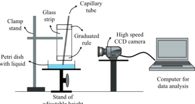
Figure 2 depicts the experimental setup that can be used for an undergraduate laboratory experience. The experimental procedure is as follows. First, assure that the glass strip attached to the clamp stand is vertical. Then, fix a capillary tube to the glass strip with plas-ticine. Take a tampered capillary tube, disinfect and pre-wet it. Knowing the glass strip length and using the graduated rules at both ends of it, measure the inclination angle β of the capillary. Prepare the liq-uid in a petri dish and put it on a stand of adjustable height. Align a high speed CCD camera and focus it on the base of the capillary tube. In order to preserve the initial condition (6), begin recording with the CCD camera, and then rise the Petri dish very slowly until the liquid starts rising into the capillary tube. In order to have enough experimental data points (n≈20), ad-just the camera speed (frames per second) and extract stills from the recorded movies (1 frame out of every 20 up to 100) depending on the liquid speed. Analyze the stills with some commercial software, converting pixel distances into mm. For this purpose it can be used as a reference the graduated rule recorded during the liquid rise. To find the inner radius of the capillary, remove the capillary from the glass strip and cut it at where it was the meniscus. Use a caliber to measure the ex-ternal radius of the capillary. Place it horizontally and zoom the camera to focus the cut end of the capillary. The image of the cross section of the capillary is then analyzed converting pixel distances into mm, with ref-erence to the external radius of the capillary previously measured.
High speed CCD camera
Stand of adjustable height
Graduated rule Glass
strip Clamp
stand
Capillary tube
Petri dish with liquid
Computer for data analysis
Figure 2 - Experimental setup for observing the liquid rise in a capillary tube.
5.
Experimental evidence
Figure 3 shows the experimental data (n = 10) of a 55% sugar solution at 25 ◦
C rising through a vertical capillary tube of radiusr= 10−4 m [10], and the error band within the theoretical curvesα(t, κfit+ ∆κfit) and
α(t, κfit−∆κfit). The experimental maximum height obtained wassexpmax = 0.123 m.According to Eqs. (24) and (25)
κfit = 5.352×10⁻³ s−1, ∆κfit = 2.859×10
−4 s−1.
According to Eqs. (26) and (27), the experimental kine-matic viscosity is
νexp±∆νexp= (1.862±0.099)×10
−5 m2s−1,
which agrees with the value given by Ref. [10], ν = 1.984×10⁻⁵ m2s−1. The adjusted coefficient of deter-mination for the non-linear fitting is [16, Eq. (3.18)]
¯
R= 0.999625,
which indicates that the fitting is quite good. The char-acteristic time for the liquid rise (19) is
texp0 = 8νexps exp max
gr2 = 188.2 s,
which is much more greater than the characteristic time for Poiseuille’s law (22),
t∗ exp=
r2
νexpλ21
50 100 150 200 250 300 t [s] 0.2
0.4 0.6 0.8
α
Figure 3 - Non-linear regression for experimental data given by [10].
Figure 4 shows the experimental data (n = 16) of water rising through a capillary tube of radius
r = 1.777 × 10⁻⁴ m, inclined an angle β = 45◦ [17], and the error band within the theoretical curves
α(t, κfit+ ∆κfit) and α(t, κfit−∆κfit). The experi-mental maximum height obtained was sexp
max = 0.1217 m.According to Eqs. (24) and (25)
κfit = 1.802×10 −1s−1, ∆κfit = 2.064×10⁻²s−1.
According to Eqs. (26) and (27), the experimental kine-matic viscosity is
νexp±∆νexp= (1.247±0.143)×10−6 m2s−1, which agrees with the value given by Ref. [18] within 10 ◦
C and 20 ◦
C (ν = 1.307×10⁻⁶ m2s−1 for 10 ◦ C and ν= 1.004×10⁻⁶ m2s−1 for 20◦
C). The adjusted coefficient of determination for the non-linear fitting is
¯
R= 0.997866,
5 10 15 20 t [s]
0.2 0.4 0.6 0.8 1.0
α
Figure 4 - Non-linear regression for experimental data given by [17].
which indicates that the fitting is also good. The char-acteristic time for the liquid rise (19) is
texp0 = 5.63 s,
which is much more greater than the characteristic time for Poiseuille’s law (22)
t∗
exp= 4.31×10 −3 s.
Figure 5 shows the experimental data (n = 22) of silicone fluid rising through a vertical capillary tube of radius r = 8.8×10⁻⁵ m, inclined an angle
β= 57.7◦
[19], and the error band within the theoretical curvesα(t, κfit+ ∆κfit) andα(t, κfit−∆κfit).The ex-perimental maximum height obtained wassexp
max= 9.25 cm. According to Eqs. (24) and (25)
κfit = 4.18×10⁻² s−1, ∆κfit = 3.90×10⁻³ s−1.
According to Eqs. (26) and (27), the experimental kine-matic viscosity is
νexp±∆νexp= (1.31±0.12)×10−6m2s−1. (28) The value given by [19] isν = 10−6 m2s−1 at 25 ◦
C. This discrepancy could be explained because of the vari-ation of viscosity with temperature. Let us assume that dynamic viscosity varies with temperature according to Andrade-Guzman equation [20, Eq. (4.15)]
η(T) =η∞exp (T
0
T
)
, (29)
where T is the absolute temperature and η∞ and T0 are parameters which depend on the liquid considered. Knowing that at T1 = 25 ◦C and at T2 = 0 ◦C the density of the silicone fluid used in the experiment is
ρ(T1) = 816 kg m−3 and ρ(T2) = 840 kg m−3, and the kinematic viscosity is ν(T1) = 10−6 m2s−1 and
ν(T2) = 1.68×10⁻⁶m2s−1 [21], then
10 20 30 40 50 60t [s]
0.2 0.4 0.6 0.8 1.0
α
η(T1) = 8.16×10⁻⁴ Pa s, (30)
η(T2) = 1.41×10⁻³ Pa s. (31) Therefore, from Eqs. (30) and (31) we may calculate the parameters of Eq. (29)
T0 = 1786 K, (32)
η∞ = 2.04×10
−6 Pa s. (33)
Performing a linear interpolation of the density between
T1andT2and taking into account Eq. (29) with the pa-rameters found in Eq. (32) and Eq. (33), we may evalu-ate numerically the temperature at which the kinematic viscosity should be Eq. (28), obtaining a temperature for the experiment ofTexp= (11.6±4.5)◦C.
The adjusted coefficient of determination for the non-linear fitting is
¯
R= 0.997757,
which indicates that the fitting is good. The character-istic time for the liquid rise (19) is
texp0 = 23.9 s,
which is much more greater than the characteristic time for Poiseuille’s law (22)
t∗
exp = 1.02×10 −3 s.
References
[1] M.G.C. Peiris and K. Tennakone, Am. J. Phys.48, 497 (1980).
[2] G.K. Batchelor, An Introduction to Fluid Dynamics (Cambridge Univ. Press, Cambridge, 1967).
[3] A.A. Elkarim, Am. J. Phys.16, 489 (1948).
[4] F.H. Hibberd, Am. J. Phys.20, 134 (1952).
[5] D.A. Barry, J.Y. Parlange, G.C. Sander and M. Siva-plan, Journal of Hydrology142, 29 (1993).
[6] N. Fries and M. Dreyer, Journal of Colloid and Inter-face Science320, 259 (2008).
[7] R. Lucas, Kolloid-Zeitschrift23, 15 (1918). [8] E.W. Washburn, Physical Review17, 273 (1921). [9] L.D. Landau and E.M. Lifshitz,Fluid Mechanics
(Perg-amon Press, Oxford, 1987).
[10] M.G.C. Peiris and K. Tenmakone, Am. J. Phys. 48, 415 (1980).
[11] J. Jurin, Philosophical Transactions of the Royal Soci-ety30, 739 (1717-1719).
[12] R.M. Corless, G.H. Gonnet, D.E.G. Hare, D.J. Jeffrey and D.E. Knuth, Advances in Computational Mathe-matics5, 329 (1996).
[13] R. Fazio and A. Jannelli, Applied and Industrial Math-ematics in Italy III82, 353 (2010).
[14] A. Siebold, M. Nardin, J. Schultz, A. Walliser and M. Oppliger, Colloids and Surfaces A161, 81 (2000). [15] E.W. Weisstein, http://mathworld.wolfram.com/
LeastSquaresFitting.html.
[16] S. Chatterjee, A. Hadi and B. Price,Regression Anal-ysis by Example (Wiley, New York, 2000).
[17] W.E. Brittin, Appl. Phys.17, 37 (1946).
[18] D.R. Lide, Handbook of Chemistry and Physics (CRC Press, Florida, 2013), 94th
ed.
[19] M. Stange,Dynamik von Kapillarstr¨omungen in Zylin-drischen Rohren (Cuvillier, G¨ottingen, 2004).
[20] D.S. Viswanath, T.K. Ghosh, D.H.L. Prasad, N.V.K. Dutt and K.Y. Rani,Viscosity of Liquids. Theory, Es-timation, Experiment, and Data(Springer, Dordrecht, 2007).
![Figure 4 shows the experimental data (n = 16) of water rising through a capillary tube of radius r = 1.777 × 10 − 4 m, inclined an angle β = 45 ◦ [17], and the error band within the theoretical curves α (t, κ fit + ∆κ fit ) and α (t, κ fit − ∆κ fit )](https://thumb-eu.123doks.com/thumbv2/123dok_br/18933991.439834/5.892.94.842.814.1079/figure-experimental-rising-capillary-radius-inclined-theoretical-curves.webp)
