An Analytical Closed-Form Lower-Bound on
Ergodic Capacity of Correlated Rayleigh-Fading
MIMO Channels
Antonio Alisson P. Guimarães and Charles Casimiro Cavalcante
Wireless Telecommunication Research Group (GTEL)Federal University of Ceará (UFC)
Campus do Pici, Bl. 722, C.P. 6005, CEP 60.455-900, Fortaleza-CE, Brazil E-mail: {alisson,charles}@gtel.ufc.br
Phone/Fax: +55-85-33669470
Abstract—In this paper, the ergodic capacity of multiple an-tenna systems over spatially correlated Rayleigh-fading channels is investigated under the assumption that the channel state information (CSI) is unknown at the transmitter and perfectly known at the receiver. We derive a lower-bound expression, in closed form, for the ergodic capacity through the use of majorization theory and the probability density function (PDF) of the sum of Gamma random variables, which is represented by an infinite series. Furthermore, we also obtain other lower-bounds from the truncation of such series, and we associate truncation errors. Finally, the proposal of the paper is compared with a lower-bound reported in the literature.
I. INTRODUCTION
In recent years, the ergodic capacity of single-user multiple-input multiple-output (MIMO) communications over flat-fading wireless channels have been exhaustively explored under different fading conditions and distinct types of spatial correlation [1]–[10]. However, to obtain analytical closed-form expressions for the ergodic capacity, especially in cor-related MIMO fading channels, is still a great challenge due to difficulty in manipulating the non-Gaussian joint channel statistics. Thus, one resorts to bounding techniques, whose bounds (lower or upper) should be as close as possible to the empirical ergodic capacity obtained through Monte Carlo methods. In particular, Zhong et al. [9], [10], by virtue of some results of majorization theory [11], have obtained upper and lower capacity bounds for Nakagami-m MIMO fading channels.
Rayleigh distribution is a fading model, which is frequently used to model the short-term behaviour of mobile-radio sig-nals [12]. In other words, the envelope of the received complex low-pass signal can be modeled as a random variable with a Rayleigh distribution for non-light-of-sight (NLoS) propa-gation. Several works, operating in Rayleigh-fading MIMO systems, have been published about analytical closed-form expressions for lower-bounds to the ergodic capacity. In [3], a lower-bound for independent and identically distributed (i.i.d.)
The authors would like to thank CAPES, CNPq (Grant No. 30677/2011-9), BNB and PRONEX/FUNCAP for the partial financial support.
flat-fading channels was derived, while [4] has been analyzing the frequency-selective fading case. In [6], tight upper and lower bounds on the ergodic capacity for spatially correlated channels were provided. The spatial double-sided correlation with keyhole has been examined in [5]. Newly, tight bounds for spatially correlated Rician MIMO channels were proposed by [7], [8] at any signal-to-noise ratio (SNR) and for any number of receive and transmit antennas. Moreover, these ref-erences devote a significant part to the study of the Rayleigh-fading channels as a particular case.
In this paper, capitalizing on the technique of [9], we analyze the ergodic capacity of spatially correlated Rayleigh-fading MIMO channels based on the Unitary-Independent-Unitary (UIU) formalism [13], [14]. Specifically, through the use of majorization theory and the distribution of the sum of Gamma random variables [15], we derive an analytical closed-form lower-bound for the ergodic capacity assuming that the channel state information (CSI) is available only at the receiver. It is important to mention that our proposal distinguishes from previous results, on Rayleigh-fading MIMO channels, due to the use of majorization theory on the Unitary-Independent-Unitary formulation applied to Kronecker chan-nel model.
The remaining parts of this paper are organized as follows. Section II presents briefly the Rayleigh and Gamma distribu-tions. Furthermore, we list some results on majorization theory. In Section III, we introduce the Rayleigh-fading MIMO chan-nel model. We derive an analytical lower-bound to the ergodic capacity in Section IV. The theoretical and the simulation results are discussed in Section V. Finally, we conclude the paper in Section VI.
The notations used throughout this paper are as follows. All matrices and vectors will be represented by bold uppercase and lowercase letters, respectively. We useIorIp for the identity
matrix of dimensionp×p,Cm×n indicates them×ncomplex
vector space and diag (·) represents a diagonal matrix. The
superscripts(·)T and(·)H denote the transpose and Hermitian
transpose, respectively. The subscript(·)i is the i-th element
operators⊙,≺andE{·}denote the Schur-Hadamard product, majorization relation, and statistical expectation, respectively. The operator det(·) stands for the determinant of a square matrix. Finally, the vectors d(·) and λ(·) denote the main
diagonal elements and eigenvalues of a Hermitian matrix, respectively.
II. PRELIMINARIES
This section presents the basic notion of majorization theory. There is an extensive list of properties involving the majoriza-tion theory, which can be found in the classical reference [11]. However, we selected some important results, which will be used in Section IV. Additionally, in this section, we provide a brief review of the statistical distributions Rayleigh and Gamma, and we present the sum of independent Gamma variables with different parameters.
A. Majorization theory
Definition 1 ( [11, 1.A.1]): For any vectors x and y in Rn×1,xis said majorized byy, denoted by,x≺y, if
k X
i=1
x[i] ≤
k X
i=1
y[i], 1≤k≤n−1 (1)
n X
i=1
x[i] =
n X
i=1
y[i]. (2)
where x[i] and y[i] denote the i-th largest components of x
andy, respectively.
Lemma 1 ( [10, Example 2]): Let x= (x1, x2, · · · , xn)
and s= (S, 0, · · · , 0) be vectors in Rn. IfS =Pn
i=1xi,
thenx≺s.
Definition 2 ( [11, 3.A.1]): A real-valued functionφ(·)on Rn×1 is said to be Schur-concave if φ(x) ≥ φ(y) for any x≺y.
Lemma 2 ( [11, 3.C.1]): Letφ(·)be a real-valued function on Rn×1. If g : R → R is concave, then φ(·) defined by
φ(x) = Pni=1g(xi)is Schur-concave.
Example 1 ( [10, Appendix II]): The real-valued function on Rn×1 φ(·), defined byφ(x) =Pn
i=1log2(1 +αxi), with α >0, is a Schur-concave function.
B. The Rayleigh and Gamma distributions
Definition 3 ( [16]): Consider X and Y two independent
zero mean Gaussian random variables with same varianceσ2.
The envelopeR=√X2+Y2is Rayleigh distributed, and the
probability density function (PDF) is given by
pR(r) = r σ2exp
− r
2
2σ2
u(r), (3)
where u(·) is the unit step function. We will use the short-hand notationR∼Rayleigh(σ2), to denote thatRis Rayleigh
distributed with parameterσ2.
Definition 4 ( [16]): A random variable X follows a
Gamma distribution with parameters α > 0 and β > 0, denoted byX ∼ γ(α, β), if the PDF ofX is given by
pX(x) =
xα−1exp (−x/β)
βαΓ(α) u(x), (4)
whereΓ(·)stands for the gamma function.
Lemma 3: IfX∼Rayleigh(σ2), then the random variable
Y =kX2 has a Gamma distribution with parameters α= 1
andβ= 2kσ2, i.e., Y ∼γ(1,2kσ2).
Now, we present the distribution of the sum ofm indepen-dent Gamma variables with parametersαmandβm. Proposed
by Moschopoulos [15], this result is expressed by an infinite series, as it will be shown in the sequel.
Lemma 4 ( [15]): Let{Xi}mi=1 be a set ofmindependent
Gamma random variables such asXm∼γ(αm, βm), then the
PDF ofY =Pmi=1Xi is given by
pY(y) =η
∞
X
k=0
δk yµ+k−1exp (−y/β∗)
Γ(µ+k)β∗µ+k
u(y), (5)
whereβ∗= min
1≤k≤m{βk},η = m Y
k=1
β
∗
βk αk
andµ=
m X
k=1
αk.
In addition, the coefficientsδi can be obtained recursively by
δ0= 1,
δk+1= 1
k+ 1
k+1
X
l=1
m X
j=1
αj
1−ββ∗ j
l δk+1−l
(6)
wherek= 0,1,2,· · ·.
III. SYSTEMMODEL ANDCHANNELCAPACITY We focus our study on single-user MIMO communications over flat-fading wireless channels withnT transmit antennas,
and nR receive antennas. The input-output relationship is
given by
y=Hx+n, (7)
where y ∈ CnR×1 and x ∈ CnT×1 are the received and transmitted signal vectors, respectively, while n∈CnR×1 is the complex additive white Gaussian noise (AWGN) vector with zero mean and covariance matrixEnnH =N
0I. We
assume that the transmitted signal vector satisfies the power constraint ExHx ≤ PT. In addition, H ∈ CnR×nT is
the MIMO channel matrix, whose elements hij represent the
complex fading parameter between thej-th transmit and i-th receive antenna.
The channel gain is considered to undergo Rayleigh-fading with spatial correlation occurring at both ends of the MIMO link, and we also assume that the channel matrix H is modeled according to the Kronecker model [17] to describe the correlation between the elements. Thus
H=R1R/2 xHw(R
1/2
Tx)
H,
(8)
where the entries of the matrixHw= [ehij]are i.i.d. complex
Gaussian random variables with zero mean and unit variance. The matricesRRx ∈C
nR×nRandR
Tx ∈C
nT×nT denote the
receive and transmit correlation matrices and their respective eigen-decomposition can be given by
RRx=URxΛRxU
H
Rx and RTx=UTxΛTxU
where URx and UTx are deterministic unitary matrices. In turn, ΛRx
△
= diag (λR
x)andΛTx
△
= diag (λT
x)are diagonal matrices containing the non-zero eigenvalues of RRx and RTx, respectively, where
λR x
△
=
λRx
1
λRx
2
.. .
λRx
nR
and λTx
△
=
λTx
1
λTx
2
.. .
λTx
nT
. (10)
A. Unitary-Independent-Unitary model
Substituting the eigenvalues decomposition for RRx and RTx (see Eq. (9)) in Eq. (8), can to express the MIMO channel matrix Husing the UIU-model [13], [14], [18] as follows
H=URx(G⊙Hw)U
H
Tx, (11)
where G is a given (deterministic) matrix coupling matrix, and the operator ⊙ is the element-wise Schur-Hadamard multiplication. Therefore, for the Kronecker channel model described in Eq. (8), the coupling matrixGis given by
G=λ1/2 Rx
λ1/2
Tx
T
, (12)
where the vectorsλ1/2 Rx andλ
1/2
Tx are the element-wise square root ofλR
x andλTx, respectively.
B. MIMO Channel Capacity
In the sequel, we consider that the receiver has perfect channel state information (CSI), and an equal-power allocation across the transmit antennas. In this situation, the ergodic capacity can be expressed as [8]
C=E
log2
det
I+ ρ
nT
Γ
, (13)
whereρ=△ PT
N0 is the received signal-to-noise (SNR) ratio and Γ is the Wishart matrix, which is defined as
Γ=
(
HHH, nR≤nT
HHH, nR> nT.
(14)
Now, we definer= min{nR, nT}andt= max{nR, nT}.
Hence,Γis always a square matrix of orderr×r. Moreover, we also assume that the number of receive antennas does not exceed the number of transmit antennas. Thus, the identity det (I+AB) = det (I+BA)ensures that all results on the ergodic capacity can be extended to the casenR> nT. Finally,
based on these assumptions, we conclude that the MIMO channel capacity in Eq. (13) can be expressed as
C=E
log2
det
InR+ ρ nT(
G⊙Hw)(G⊙Hw)H
(15)
IV. LOWER-BOUND ONERGODICCAPACITY In this section, we derive a closed-form expression, in terms of the Meijer G-function [19, Eq. (9.301)], for the lower-bound on the ergodic capacity using some results of majorization theory and the distribution of the sum of independent Gamma random variables. The details are presented in the following theorem.
Theorem 1: The ergodic capacity of spatially correlated Rayleigh MIMO channels is lower bounded by
C ≥ln 2η
∞
X
k=0
δk
Γ(rt+k)G 1,3 3,2
ρβ∗
nT
1−rt−k,1,1
1,0
, (16)
whereρis the SNR, the constantβ∗= min
n λRx
i λ
Tx
j o
and
Gm,np,q (· | ·)is the Meijer G-function. Moreover, the constant η is given by
η =
r Y
i=1
t Y
j=1
β∗
λRx
i λ
Tx
j
, (17)
and the coefficientsδk is obtained recursively by
δ0= 1,
δk+1 = 1
k+ 1
kX+1
l=1
δk+1−l
r X
i=1
t X
j=1
1− β∗ λRx
i λ
Tx
j !l
(18) wherek= 0,1,2,· · ·.
Proof: Firstly, for convenience, we define the matrix W=△ G⊙Hw and the following vectors inRr×1:
dWWH= (△ d1, d2, · · · , dr), (19a)
λWWH= (△ λ1, λ2, · · · , λr) and (19b)
Λ=△
r X
i=1
λi, 0, · · ·, 0 !
, (19c)
where di corresponds to the i-th diagonal element of the
Hermitian matrix WWH, and λi represents the respective
eigenvalue. Now, let be the real-valued functionφ(·)onRr×1
defined by
φ(x) =
r X
i=1 log2
1 + ρ
nT xi
. (20)
From Lemma 1, we have that the vector Λ majorizes
λWWH, i.e., λWWH ≺Λ. Since φ(·) is a Schur-concave function (see Example 1), we obtain the following nu-merical inequality:φλWWH≥φ(Λ). Now, applying the expectation operatorE{·}, in this inequality, and observing that the ergodic capacity presented in Eq. (15) is equal to EnφλWWH o, that is,
C=E
( r X
i=1 log2
1 + ρ
nT λi
)
we obtain a lower-bound to the ergodic capacity as shown below:
C ≥ Clo=E
log2
1 + ρ
nT r X
j=i λi
. (22)
According to the singular value decomposition (SVD) of the matrixWWH, we ensure thatPri=1λi=Pri=1di. Thus, the
lower-boundClo can be equivalently written as
Clo= 1 ln 2
Z ∞
0
G12,,22
ρ nT
s1,1
1,0
pS(s)ds, (23)
wherepS(·)is the PDF of the random variable S △
=Pri=1di
andln (1 +ks)is equal toG12,,22
ks1,1
1,0
[10]. Now, note that
S=
r X
i=1
t X
j=1
λRx
i λ
Tx
j |ehij|2. (24)
In other words, the variableSis a sum of independent Gamma variables. Specifically,λRx
i λ
Tx
j |ehij|2∼γ
1, λRx
i λ
Tx
j
. Thus, based on Lemma 4, the PDFpS(·) is given by
pS(s) =η
∞
X
k=0
δk srt+k−1exp (−s/β∗)
Γ(rt+j)β∗rt+j
u(s), (25)
whereβ∗= min
n λRx
i λ
Tx
j o
and the parametersη andδi are
described in Eq. (17) and (18), respectively. Now, substituting the PDFpS(·)into Eq. (23) and using the fact [19, Eq.
(7.813-1)], [10]
Z ∞
0
x−ρexp (
−βx)Gm,n p,q
αxa
1,a2,···,ap
b1,b2,···,bq
dx=
βρ−1Gm,n+1
p+1,q α
β
ρ,a1,a2,···,ap
b1,b2,···,bq
, (26)
we conclude, after some algebra, that the lower-bound Clo is given by Eq. (16). This completes the proof.
Though the lower-bound obtained can be expressed in an analytical closed-form expression, and can be evaluated very efficiently using standard softwares like MAPLE and MATHEMATICA, for practical numerical evaluations, we con-sider a truncated version of the infinite series in Eq. (25), and we associate it an approximation error of the area under the PDF pS(·). Specifically, we define the truncated version
of the infinite series in Eq. (25), with an arbitrary truncation parameterL, as follows:
pS(s, L) =η L X
k=0
δk srt+k−1exp (−s/β∗)
Γ(rt+j)β∗rt+j
u(s). (27)
Then, repeating the procedures given in Theorem 1, we have the following lower-bound to the ergodic capacity:
Clo(L) = η ln 2
L X
k=0
δk
Γ(rt+k)G 1,3 3,2
ρβ
∗
nT
1−rt−k,1,1
1,0
. (28)
Now, in order to find a criterion that allows to identify the values of L, which provides a good truncation factor of the
infinite series described in (25), we analyze the approximation error of the area under the PDF pS(·) from the following
functionE(·):
E(L)=△
Z ∞
0
pS(s)ds− Z ∞
0
pS(s, L)ds. (29)
Note that,
E(L) = 1−η L X
k=0
δk
Γ(rt+k)β∗rt+k
× Z ∞
0
srt+k−1exp (
−s/β∗)u(s)ds. (30)
Applying the integration result [19, Eq. (8.312-2)] in Eq. (30)
Z ∞
0
tz−1exp (−kt)dt= Γ(z)
kz , (31)
we obtain
E(L) = 1−η L X
k=0
δk. (32)
Hence, we conclude that, if the approximation error E(·) is sufficiently small, then the area under the curve given by
Clo(·)is sufficiently close to the area under lower-boundClo. Consequently, we obtain a good approximation to the ergodic capacity. The numerical details about truncation factorLand the approximation errorE(·)are described in Section V.
V. NUMERICALRESULTS
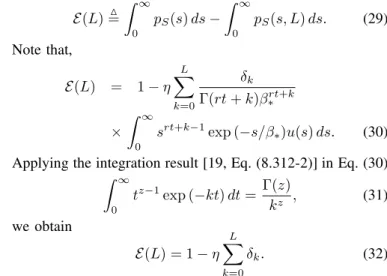
In order to illustrate the theory described in Section IV, we evaluate in this section the ergodic capacity lower-bounds for a number of different cases, assuming the exponential correlation model [8] with receive and transmit correlation coefficients equal to δRx = 0.3 andδTx = 0.5, respectively. Moreover, we compare our lower-bound with McKay and Collings [7, Section IV] whose reference investigates the Rayleigh-fading channels as a particular case of Rice-fading channels.
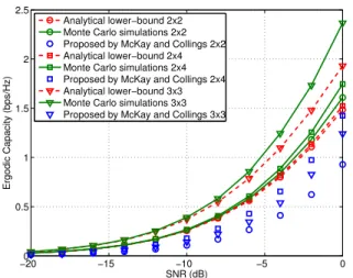
Fig. 1 gives the truncation errors of the area under the PDF
pS(·) obtained in Eq. (25). Consequently, the convergence
speed of the simulated curves. Thus, from the choice of a specific error factor, we have an effective criterion for determination of the associated truncation factor. Thus, for an errorE = 1−10−3, we obtain different truncation factors as
summarized in Table I.
TABLE I
TRUNCATION FACTORS FOR DIFFERENT SCENARIOS Channel 1×1 1×2 1×4 2×2 2×4 3×3
0 20 40 60 80 100 0
0.1 0.2 0.3 0.4 0.5 0.6 0.7 0.8 0.9 1
Truncation factor (L)
Approximation error of the area under PDF p
S
(.)
Channel 1x1 Channel 1x2 Channel 1x4 Channel 2x2 Channel 2x4 Channel 3x3
Fig. 1. Approximation error of the area under the PDFpS(·).
−200 −15 −10 −5 0 5 10 15 20
1 2 3 4 5 6 7
SNR (dB)
Ergodic Capacity (bps/Hz)
Analytical lower−bound 1x1 Monte Carlo simulations 1x1 Proposed by McKay and Collings 1x1 Analytical lower−bound 1x2 Monte Carlo simulations 1x2 Proposed by McKay and Collings 1x2 Analytical lower−bound 1x4 Monte Carlo simulations 1x4 Proposed by McKay and Collings 1x4
Fig. 2. Comparison of the empirical ergodic capacity and analytical lower-bounds to the ergodic capacity for1×1,1×2and1×4correlated
Rayleigh-fading channels.
−200 −15 −10 −5 0
0.5 1 1.5 2 2.5
SNR (dB)
Ergodic Capacity (bps/Hz)
Analytical lower−bound 2x2 Monte Carlo simulations 2x2 Proposed by McKay and Collings 2x2 Analytical lower−bound 2x4 Monte Carlo simulations 2x4 Proposed by McKay and Collings 2x4 Analytical lower−bound 3x3 Monte Carlo simulations 3x3 Proposed by McKay and Collings 3x3
Fig. 3. Comparison of the empirical ergodic capacity and analytical lower-bounds to the ergodic capacity for2×2,2×4and3×3correlated
Rayleigh-fading channels.
VI. CONCLUSIONS
We have investigated the ergodic capacity of MIMO sys-tems operating on spatially correlated Rayleigh-fading chan-nels, assuming the UIU-decomposition. From some results on majorization theory, we have derived an analytical closed-form lower-bound to ergodic capacity. Additionally, we have derived other lower-bounds from the truncated version of the infinite series described by the PDF of the sum of Gamma random variables. In addition, from the analytical lower-bound obtained, we have associated an approximation error in terms of the area under of such PDF. Finally, we have verified that our lower-bound is tighter than previously known analytical lower-bound, in the low-SNRs, while for MISO systems, all results are equally tight.
REFERENCES
[1] I. E. Telatar, “Capacity of multi-antenna Gaussian channels,” Europ. Trans. Telecommun., vol. 10, no. 6, pp. 585–595, Nov. 1999. [2] G. J. Foschini and M. J. Gans, “On limits of wireless communications
in a fading environment when using multiple antennas,” Wireless Pers. Commun., vol. 6, pp. 311–335, 1998.
[3] A. Grant, “Rayleigh fading multi-antenna channels,” EURASIP Journ. Wireless Commun. and Networking, vol. 3, pp. 316–329, 2002. [4] O. Oyman, R. Nabar, H. Bölcskei, and A. Paulraj, “Tight Lower Bounds
on the Ergodic Capacity of Rayleigh Fading MIMO Channels,” inProc. of IEEE Global Telecommunications Conference (GLOBECOM), Nov. 2002, vol. 2, pp. 1172–1176.
[5] X.W. Cui and Z.M. Feng, “Lower Capacity Bound for MIMO Correlated Fading Channels with Keyhole,”Communications Letters, IEEE, vol. 8, no. 8, pp. 500 – 502, aug. 2004.
[6] Q.T. Zhang, X.W. Cui, and X.M. Li, “Very Tight Capacity Bounds for MIMO-Correlated Rayleigh-Fading Channels,” IEEE Trans. Wireless Commun., vol. 4, no. 2, pp. 681–688, Mar. 2005.
[7] M. R. McKay and I. B. Collings, “General Capacity Bounds for Spatially Correlated Rician MIMO Channels,” IEEE Trans. Inform. Theory, vol. 51, no. 9, pp. 3121–3145, Sept. 2005.
[8] S. Jin, X. Gao, and X. You, “On the Ergodic Capacity of Rank-1 Ricean-Fading MIMO Channels,” IEEE Trans. Inform. Theory, vol. 53, no. 2, pp. 502–517, Feb. 2007.
[9] C. Zhong, K-K. Wong, and S. Jin, “On the Ergodic Capacity of MIMO Nakagami-Fading Channels,” in IEEE Int. Symp. on Inform. Theory (ISIT), July 2008, pp. 131 –135.
[10] C. Zhong, K-K. Wong, and S. Jin, “Capacity Bounds for MIMO Nakagami-m Fading Channels,” IEEE Trans. Signal Processing, vol.
57, no. 9, pp. 3613–3623, Sept. 2009.
[11] A. W. Marshall and I. Olkin, Theory of Majorization and Its Applica-tions, Academic Press, 1979.
[12] W. C. Lee, Mobile Communications Engineering, McGraw-Hill, 2 edition, 2008.
[13] W. Weichselberger, M. Herdin, H. Ozcelik, and E. Bonek, “A Stochastic MIMO Channel Model With Joint Correlation of Both Link Ends,”IEEE Trans. Wireless Commun., vol. 5, no. 1, pp. 90 – 100, Jan. 2006. [14] A.M. Tulino, A. Lozano, and S. Verdu, “Impact of antenna correlation
on the capacity of multiantenna channels,” IEEE Trans. Inform. Theory, vol. 51, no. 7, pp. 2491–2509, July 2005.
[15] P. G. Moschopoulos, “The distribution of the sum of independent gamma random variables,”Annals of the Institue of Statistical Mathematics, vol. 37, pp. 541–544, 1985.
[16] V. Krishnan, Probability and random processes, John Wiley & Sons, Inc., 2006.
[17] V. Raghavan, J.H. Kotecha, and A.M. Sayeed, “Why Does the Kronecker Model Result in Misleading Capacity Estimates?,” IEEE Trans. Inform. Theory, vol. 56, no. 10, pp. 4843 –4864, Oct. 2010.
[18] G. Rafiq., V. Kontorovich, and M. Patzold, “On the Statistical Properties of the Capacity of Spatially Correlated Nakagami-mMIMO Channels,”
inIEEE Veh. Technol. Conference, May 2008, pp. 500–506.