Maria Cecilia Goi Porto AlvesI
Nilza Nunes da SilvaII
I Instituto de Saúde. Secretaria de Estado da Saúde de São Paulo. São Paulo, SP, Brasil
II Departamento de Epidemiologia. Faculdade de Saúde
Pública. Universidade de São Paulo. São Paulo, Brasil Correspondence:
Maria Cecilia Goi Porto Alves R. Santo Antônio, 590 – 5º. Andar 01314-000 São Paulo, Brasil E-mail: [email protected] Received: 3/9/2007
Approved: 7/30/2007
Variance estimation methods in
samples from household surveys
ABSTRACT
OBJECTIVE: Knowledge of sampling errors is essential for correctly
interpreting the results from household surveys and evaluating their sampling designs. The composition of household samples used in surveys gives rise to situations of complex estimation. In this light, the study was conducted with the aim of evaluating the performance of the variance estimators in surveys carried out among urban populations in Brazil.
METHODS: The reference population was the sample drawn by the Fundação
Sistema Estadual de Análise de Dados Estatísticos (SEADE – State Statistical Data Analysis System Foundation) for carrying out an employment and unemployment survey in the metropolitan region of São Paulo. Three techniques were used for estimating variance: Taylor linearization and Jackknife and BRR replication. Repeated samples were selected from the reference population, using stratifi ed cluster sampling in two stages (census tracts and households). Three different designs were used and 2,000 samples were drawn within each design. To obtain an estimator ratio, the accuracy of the variance estimators was evaluated by means of the mean square error and the confi dence interval coverage.
RESULTS: According to the mean square error, the three techniques provided
similar accuracy. The bias ratios were approximately 0.10, for the smaller samples. The confi dence interval coverage indicated that the confi dence levels observed were lower than what was set (95%), and were around 90% for the smaller samples.
CONCLUSIONS: The variance estimators showed similar performance
with regard to accuracy and confi dence interval coverage. The bias was irrelevant in relation to the magnitude of the standard error. Although the real confi dence levels were lower than the nominal levels for normal distribution, the changes did not prevent construction of interval estimates with reasonable confi dence.
KEY WORDS: Estimation techniques. Data collection. Stratifi ed sampling. Cluster sampling. Taylor series linearization. Complex sample design.
INTRODUCTION
Knowledge of sampling errors is essential for correctly interpreting the results from household surveys and evaluating their sampling designs.16 However,
the composition of household samples with multi-stage cluster draws makes estimation complex. In such cases, the ordinary approach of using variance estimation methods based on simple random sampling (SRS) can be regarded as inappropriate.9
in the sample, yi is the value of these elements and
is its mean.8
In household surveys, because the population elements are scattered over wide geographic areas, it becomes necessary to use cluster sampling in order to reduce the cost of data collection. By using clusters with differing sizes and self-weighted sampling procedures, the num-ber of sample memnum-bers becomes a random variable, which transforms the mean into a ratio of variables, with consequences for estimating the sampling error. In this context, the majority of fi rst-order estimators are nonlinear, and because there are no exact expressions for calculating their variances, it becomes necessary to use approximations adjusted to the complex nature of the sampling design and the estimation procedure. Nowadays, the most frequently used methods for estimating variance in complex sampling designs are Taylor-series linearization and replication. The fi rst pro-vides a linear approximation for the nonlinear estimator of interest, by means of the Taylor series, to which the usual linear estimator formulas are applied. In order to obtain an adequate approximation for the variance of the ratio estimator by means of a Taylor series, the sample size (the denominator of the ratio) should not be subject to great variation, which would however be the case when the clusters have widely different sizes. The diffi culty in keeping the denominator variability under control increases if the estimation is directed to-wards subclasses, since it is then impossible to control the number of units belonging to each subclass. This is especially true for phenomena that are rare and/or unevenly distributed throughout the clusters.
For the ratio estimator, , the variance estimator expression obtained by using the Taylor linearization method has been widely used in sampling, and it is as
follows: .8
In spite of being frequently presented in the literature on statistics, this expression cannot be regarded as simple from a computational standpoint, since it requires the numerator variance, var(y), the denominator variance, var(x) and their covariance, cov(x,y).
Replication techniques were developed as a simplifying alternative approach towards the variance estimation procedure. They consist of obtaining subsets from the full sample (replicate samples), repeating the estima-tion procedure for each subsample and calculating the variance from these estimates. Therefore if θis the parameter of interest and its estimator, K replicates are formed and estimates are obtained for each replicate
using . The variance estimator for is given by: , where c is a constant associated with the replication method adopted.17
This construction follows the simplicity of variance estimation found in SRS, which uses the deviations of each observation from the mean. The basic concept was developed by Mahalanobis in studies in 1944 and 1946, in which the use of replicate samples called “interpen-etrating samples” was proposed to make it easier to es-timate sampling errors and to investigate non-sampling errors such as bias related to interviewers.7
The most common replication techniques are “Bal-anced Repeated Replication” (BRR) and “Jackknife”. BRR was developed as an estimation alternative for designs that, for effi ciency reasons, use a large number of strata and consequently the least possible number of primary sampling units for each stratum, i.e. two units. It originated from the pseudo-replication scheme known as “half-sample replication”, which was proposed by the United States Bureau of the Census and later adapted and modifi ed by experts from the National Center of Health Statistics. In 1966, McCarthy12 introduced the balancing
referred to in the name of the technique. The replicates are composed of one sampling units from each stratum. In the Jackknife technique, each replicate is obtained by successively omitting one sampling unit from each stratum. Jackknife estimation procedures were origi-nally developed by Quenouille, in 1949, with the pur-pose of reducing the bias of the correlation coeffi cient estimator in time series. Tukey15 suggested that the individual estimators from the subsamples created by this technique could be seen as independent and identi-cally distributed random variables, thereby yielding a very simple variance estimator. He named it Jackknife in reference to the multipurpose tool of the same name. Its use in the context of fi nite populations seems to have been considered for the fi rst time by Durbin, in 1959, in connection with the ratio estimator.18
Besides providing simpler variance expressions than those obtained by the Taylor linearization method, one attractive feature of replication techniques is that, for a given design, the same analysis procedure is used for almost all statistics, regardless of their complex-ity. Another property of replication techniques is that they enable users of secondary survey data to estimate sampling errors without knowing the detailed sample design. The replicates created by the investigators in-volved in the survey can simply be used and included in the data fi le. This is especially useful when there are confi dentiality issues involving the sample units and it is necessary to avoid dissemination of any information identifying the sample units.14,*
Present-day electronic processing capabilities make it possible to apply any of these techniques for estimat-ing samplestimat-ing errors in surveys designed with cluster sampling. The comparative studies available are based on empirical results obtained in various countries under different designs.1,3,4,9,10,13
The present study had the objective of showing the performance of the Jackknife, BRR and Taylor linear-ization techniques for variance estimation, in samples that refl ect the sociodemographic structure of the metro-politan region of São Paulo. With this aim, census tract samples (which form the geographic units most used in household surveys in Brazil) were used to compare the accuracy of variance estimators. Through this, the intention was to contribute towards the knowledge and dissemination of the alternatives for sampling error estimation that exist, and thus to stimulate the use of adequate techniques for making statistical inferences from household surveys.
METHODS
The reference population for developing the study was a sample drawn by the Fundação Sistema Estadual de Análise de Dados Estatísticos (SEADE - State Statis-tical Data Analysis System Foundation) for carrying out an employment and unemployment survey in the metropolitan region of São Paulo.6
Repeated samples were taken from this population, using stratifi ed cluster sampling in two stages. The census tracts constituted the primary sampling units (PSUs) and the households were the secondary units. From each stratum, two census tracts were drawn with probability proportional to the number of households. From each of these census tracts, fi ve households were drawn, thus totaling ten households per stratum. The sampling fraction for stratum h was given by: , where Mh is the number of households in stratum h and Mhα is the number of households in census tract α of stratum h.
In order to evaluate the accuracy of the variance estima-tors in relation to increases in the number of primary sampling units, three designs were defi ned, without
changing the general model presented previously. For the fi rst, second and third designs, the population was organized into 8, 16 and 32 strata respectively. After drawing two census tracts per stratum, the numbers of tracts included in the samples were 16, 32 and 64. Also taking into account that fi ve households were drawn in each tract, the fi nal sample sizes in the three designs were 80, 160 and 240 households.
A total of 2,000 total of samples were drawn under each design.
The estimated mean family income was for each sample, by using the following expression: ,
where yhαβis the family income of the household β, belonging to census tract α, in stratum h; xhaβ =1, for households with income and xhaβ =0 for those with no response; wh =1/ƒh , the weight of each household, is given by the inverse of the sampling fraction of the stratum that the household belongs to, ƒh =10/Mh. From the frequency distribution, the population variance
was calculated for each design:
where E(r) is the expected value of r corresponding to
the mean of its sampling distribution, , and
ri is the mean income calculated for the i-th sample. Variance estimates using the Jackknife and BRR techniques were calculated using the WesVar soft-ware, version 4.0,17 according to the expression:
, where r is an estimate based on all the primary units; r(g) is an estimate based on the g-th replicate; G is the number of replicates and c is a constant that depends on the replication technique, (c=G for BRR; c=1 for Jackknife).
where ah =2 , i.e. the number of primary sampling units;
wha is the weight of household α in stratum h; yha is the value of the study variable in household α in stratum h; xhα=1 if there is information on the household and
xhα=0 if not.
Considering that the accuracy refers to small total errors, including bias and sampling variability, the accuracy of the estimators was evaluated by means of the mean square error: MSE[var(r)] = Var[var(r)+Bias2[var(r)] and by
means of its relative measure: .9
The sampling distribution variance was expressed by:
, and E[var(r)], i.e. the expected value for the variance of r, was
calcu-lated as follows: .1
The bias of the estimators, measured as the dis-tance between the means of the sampling distri-bution and of the population, was expressed by:
Bias[var(r)] = E[var(r)] – S2, for which the terms were
presented earlier. The effect of the bias on the accu-racy of the estimators was evaluated by the bias ratio, which measures the bias in standard deviation units:
.9
The distribution of the standardized ratio was studied with a view to checking the real confi dence level of the constructed intervals. Using Student’s t distribution values for 8, 16 and 24 degrees of freedom, the following intervals were respectively constructed: [-2.306;+2.306], [-2.120;+2.120] and [-2.064;+2.064]. Next, the proportion of times that the standardized ra-tio was within the above intervals was calculated and checked for its closeness to 0.95. Because the exact distribution of the standardized ratio is unknown for complex estimators, calculation of the coverage and checking its pertinence to predetermined intervals makes it possible to evaluate the applicability of the confi dence intervals.1
RESULTS
The sampling distributions for the estimator r were constructed for each of the three designs that were defi ned, assuming that the shape of the distribution of 2,000 estimates was stable enough to be regarded as a sampling distribution. The variance of these distri-butions was taken to be the real variance of r for the fi xed design, as done by Bean and Kish & Frankel in their studies.1,9
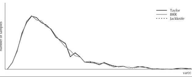
Likewise, the sampling distributions of the variance estimators for the BRR, Jackknife and Taylor tech-niques were constructed and are shown in Figures 1 to 3. Each fi gure refers to one of the sampling designs. The means and standard errors of the distributions are indicated on each fi gure.
It can be noted by overlaying the curves that the results regarding the precision and bias of the estimators were very similar. These results are shown in Table 1. According to the relative mean square error, the BRR, Jackknife and Taylor techniques provide similar ac-curacy. The differences between the measurements are only in the third decimal places, except for Jackknife in the design with 16 primary sampling units.
In the fi rst design, with 16 census tracts, the bias ratios were approximately 0.10, which means that the bias cor-responded to 10% of the standard error of the variance. The ratios decreased to approximately 0.04 and 0.06 in the designs with 32 and 48 census tracts, respectively. Table 2 shows the results regarding the inclusion of the population parameters within the calculated confi dence intervals. The observed confi dence levels were lower than the predetermined values (95%), ranging from around 90% for the samples with 16 primary sampling units to around 94% for the larger samples. The results for the three techniques were very similar.
DISCUSSION
From the sampling distributions of the variance esti-mators, a pattern was seen in relation to the standard error and bias, which were indicators of the precision, reliability and validity of the results obtained. There were small differences among the estimators, with very similar results for BRR and Taylor and slightly inferior performance by the Jackknife technique. The differences were more accentuated for the results with smaller degrees of freedom, while they ceased to ex-ist or became much smaller as the number of primary sampling units increased.
With regard to accuracy, the differences were so small that they would not have been detected had the mean square error been calculated to only two decimal places. Thus, it is hard to speak of greater accuracy for one estimator or another. Data from other studies corrobo-rate the observed similarity of the results relating to the different estimators.
Bean1 carried out an empirical investigation on the
that the latter showed slightly lower mean square errors. Kish & Frankell9 studied BRR, Jackknife and Taylor
estimators, using the data from the Current Population Survey carried out by the U. S. Bureau of the Census. The authors concluded that the variability of the Tay-lor method was the lowest, although the differences in relation to the other estimators were quite small, especially when ratio estimators were used. In terms of precision, Taylor was followed by Jackknife. Kovar et al10 compared the Taylor, BRR, Jackknife and bootstrap
estimators in a simulation study based on hypotheti-cal populations that were constructed to resemble the population in the National Assessment of Educational Progress. With regard to the precision of the variance estimates of the ratio estimator, the authors concluded that the best performances were obtained by Taylor and Jackknife, which had equal results.
By means of the bias ratio, it was noted that, for all the techniques, the bias is irrelevant when compared to the magnitude of the standard error of the variance estimates. This leads to the conclusion that, under the conditions prevailing in this study, the accuracy prob-lems of the estimators are more intensely associated with precision problems than with bias.
These results coincide with those obtained by Kish & Frankel9 and Bean,1 who concluded that there is
no consistent pattern of lower bias for any particular estimator. Rather, the bias is small and acceptable for all estimators under evaluation. Kovar et al.10 came
to the same conclusion when evaluating the bias in different situations. For designs in which two primary sampling units per stratum were drawn, they took coeffi cients of variation for the mean denominator of the r ratio that were either less than or equal to, or greater than 10%. They found that, for low coeffi cients of variation, the bias of the variance estimators was irrelevant. However, when the coeffi cient of variation for the mean denominator became greater than 10%, BRR showed considerable positive bias, whereas Jackknife and Taylor tended to slightly underestimate the real variance.
With regard to the coverage of the confi dence inter-vals, the results indicated similar performances by the three techniques, as had previously been concluded in
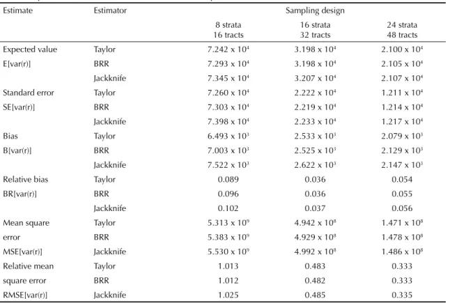
Table 1. Expected values, standard errors, bias and mean square errors of var(r).
Estimate Estimator Sampling design
8 strata 16 tracts
16 strata 32 tracts
24 strata 48 tracts
Expected value Taylor 7.242 x 10⁴ 3.198 x 10⁴ 2.100 x 10⁴
E[var(r)] BRR 7.293 x 10⁴ 3.198 x 10⁴ 2.105 x 10⁴
Jackknife 7.345 x 10⁴ 3.207 x 10⁴ 2.107 x 10⁴
Standard error Taylor 7.260 x 10⁴ 2.222 x 10⁴ 1.211 x 10⁴
SE[var(r)] BRR 7.303 x 10⁴ 2.219 x 10⁴ 1.214 x 10⁴
Jackknife 7.398 x 10⁴ 2.233 x 10⁴ 1.217 x 10⁴
Bias Taylor 6.493 x 10³ 2.533 x 10³ 2.079 x 10³
B[var(r)] BRR 7.003 x 10³ 2.525 x 10³ 2.129 x 10³
Jackknife 7.522 x 10³ 2.622 x 10³ 2.147 x 10³
Relative bias Taylor 0.089 0.036 0.054
BR[var(r)] BRR 0.096 0.036 0.055
Jackknife 0.102 0.037 0.056
Mean square Taylor 5.313 x 10⁹ 4.942 x 10⁸ 1.471 x 10⁸
error BRR 5.383 x 10⁹ 4.929 x 10⁸ 1.478 x 10⁸
MSE[var(r)] Jackknife 5.530 x 10⁹ 4.992 x 10⁸ 1.486 x 10⁸
Relative mean Taylor 1.013 0.483 0.333
square error BRR 1.012 0.482 0.333
RMSE[var(r)] Jackknife 1.025 0.485 0.335
Table 2. Coverage of the confi dence intervals constructed over 2,000 samples with Student’s t values, according to estimation method and sampling design.
Estimator Sampling design
8 strata 16 tracts
16 strata 32 tracts
24 strata 48 tracts
Taylor 90.20 93.90 94.10
BRR 90.10 93.85 93.95
Figure 1. Sampling distribution of the variance of the ratio estimator (mean 1353.955 and standard error 256.750), for the sampling design with 8 strata and 16 primary sampling units, according to variance estimation technique.
var(r)
number of samples
Taylor BRR Jackknife
Figure 2. Sampling distribution of the variance of the ratio estimator (mean 1353.767 and standard error 171.616), for the sampling design with 16 strata and 32 primary sampling units, according to variance estimation technique.
var(r)
number of samples
Taylor BRR Jackknife
Figure 3. Sampling distribution of the variance of the ratio estimator (mean 1353.107 and standard error 137.564), for the sampling design with 24 strata and 48 primary sampling units, according to variance estimation technique.
var(r)
number of samples
other studies. Although the observed confi dence levels were lower than the predetermined ones, they were always higher than 90%, even for the design that only included 16 census tracts. These changes in the confi -dence level can be regarded as tolerable.1,9 However,
for inference purposes, researchers should be aware of their existence.
Other empirical studies that evaluated the applicability of confi dence intervals to different populations, using different estimators and designs, have also found that the real confi dence levels were lower than the nominal levels of normal distribution. The authors of those studies considered that the changes did not prevent the interval estimates from being made with reasonable confi dence. In his study, Bean1 noted coverage greater
than 90% for the BRR and Taylor estimators, with results closer to 95% for the fi rst of these. For the ratio estimator, Kish & Frankel9 also found that the coverage
was best with BRR (ranging from 90.4 to 94.4%), fol-lowed by Jackknife (from 89.4 to 94.3%) and lastly by Taylor (from 88.8 to 94.0%). Kovar et al10 considered
BRR and Jackknife to be equivalent.
The results from the present study showed that the inferences were valid even for the design in which only eight census tracts were drawn. Even in surveys carried out with many primary sampling units, it may be of interest to study population subgroups that are restricted to some of these clusters. This often occurs in health surveys and it gives rise to the need to obtain interval estimates with a much lower number of pri-mary units than in the overall design. In a study on the performance of the Jackknife estimator for systematic sampling with two to 30 primary sampling units, Burke & Rust3 showed that valid inferences could be made
with samples from at least six primary units.
Taking into consideration that the methods evaluated showed equivalent results with regard to precision and bias, decisions on which estimation methods to use in health surveys will depend heavily on operational issues. Furthermore, the availability of software to calculate variance estimates under complex designs is a relevant criterion in this choice.
Various software possibilities have been developed over recent decades. Specifi c software for variance estimates using one or both of these methods has been created.5,11
Moreover, widely used data analysis software such as SAS, STATA and SPSS, has become capable of han-dling variance estimation in complex study designs, thus expanding the range of alternatives available for analyzing the data coming from household surveys.2
Efforts need to be made by the researchers responsible for conducting these surveys such that information re-lating to the sampling designs is always included in the data fi les. The basic information needed is the primary sampling units and the strata to which the study units belong, and their weights, if any.
ACKNOWLEDGEMENTS
1. Bean JA. Distribution and properties of variance estimators for complex multistage probability samples. An empirical distribution. Vital Health Stat 2. 1975;(65): i-iv,1-46.
2. Brogan D. Sampling error estimation for survey data. In: Household sample surveys in developing and transition countries. New York: United Nations Publication; 2005. p.447-90.
3. Burke J, Rust K. On the performance of Jackknife variance estimation for systematic samples with small numbers of primary sampling units. In: Proceedings of the Survey Research Methods Section, American Statistical Association. Alexandria (VA): ASA; 1995. p. 321-7.
4. Campbell C, Meyer M. Some properties of T Confi dence Intervals for Survey Data. In: Proceedings of the American Statistical Association, Survey Research Methods Section; 1978. p. 437-42.
5. Carlson BL. Software for statistical analysis of sample survey data. In: Armitage P, Colton T, editores. Encyclopedia of biostatistics. Cambridge: Harvard University; 1998 [Acesso em 15/10/2007]. Disponível em: http://www.fas.harvard.edu/~stats/survey-soft/ blveob.html
6. Fundação Sistema Estadual de Análise de Dados. Pesquisa de Emprego e Desemprego – Conceitos, Metodologia e Operacionalização. São Paulo; 1995.
7. Kalton G. Practical methods for estimating surveys sampling errors. Bull Int Statist Inst. 1977;47(3):495-514.
8. Kish, L. Survey sampling. New York: John Wiley & Sons; 1965.
9. Kish L, Frankel MR. Inference from complex samples. J
R Stat Soc Ser B Methodol. 1974;36(1):1-37.
10. Kovar JG, Rao JNK, Wu CFJ. Bootstrap and other methods to measure errors in survey estimates. Canad J
Statist. 1998;16(Supl):25-45.
11. Lepkowski J, Bowles J. Sampling error software for personal computers. Surv Stat [periódico na internet].1996[Acesso em 15/10/2007](35):10-7. Disponível em: <http://www.fas.harvard.edu/~stats/ survey-soft/iass.html>.[informar link correto]
12. McCarthy PJ. Replication: an approach to the analysis of data from complex surveys. Vital Health Stat 2. 1966;(14):1-38.
13. Mulry MH, Wolter KM. The effect of Fisher’s z-transformation on confi dence intervals for the correlation coeffi cient. In:Proceedings of the Survey Research Methods Section of the American Statistical Association; 1981. p. 601-6.
14. Skinner CJ, Holt D, Smith TMF. Analysis of complex surveys. Chichester: John Wiley & Sons; 1989.
15. Tukey JW. Bias and confi dence in not-quite large samples. Abstract. Ann Math Statist 1958;29:614.
16. United Nations. Sampling errors in household surveys. New York; 1993.
17. Westat. WesVarTM 4.0 User’s guide. Rockville: Westat;
2000.
18. Wolter KM. Introduction to variance estimation. New York:Springer-Velag; 1985.
REFERENCES
Article based on the doctorate thesis by MCGP Alves, presented to the Epidemiology Department of Faculdade de Saúde Pública of Universidade de São Paulo.