PARAFAC-Based Unified Tensor Modeling
for Wireless Communication Systems with
Application to Blind Multiuser Equalization
Andr´
e L. F. de Almeida
a,∗
G´
erard Favier
a,∗
Jo˜
ao Cesar M. Mota
baLaboratoire I3S, CNRS/UNSA
2000 Route des Lucioles, BP 121, 06903 Sophia Antipolis Cedex, France Tel: +33 4 92 94 27 36; Fax: +33 4 92 94 28 96
bWireless Telecom Research Group (GTEL), DETI/UFC
Campus do Pici, CP 6005, 60455-970, Fortaleza, Cear´a, Brazil
Abstract
In some antenna array based wireless communication systems the received signal is multidimensional and can be treated as a tensor (3D array) instead of a matrix (2D array). In this paper, we make use of a tensor decomposition known as PARAFAC (parallel factors) and propose a tensor (3D) model for the signal received by three types of wireless communication systems. The considered wireless communication systems are multiuser systems subject to frequency-selective multipath and employ-ing multiple receiver antennas together with i) oversamplemploy-ing or ii) direct-sequence spreading or iii) multicarrier modulation. The proposed modeling approach aims at unifying the received signal model of these systems into a single PARAFAC model. We show that the proposed model has a constrained structure, where model con-straints and associated dimensions depend on each particular system. The proposed PARAFAC model is demonstrated by expanding the tensor using Kronecker prod-ucts of canonical vectors. As an application of this model to tensor signal processing, a new tensor-based receiver is proposed for blind multiuser equalization, which com-bines PARAFAC-based modeling with a subspace method. Simulation results are presented to illustrate the performance of the proposed blind receiver.
Key words: Alternating least squares, antenna arrays, blind equalization,
direct-sequence spreading, frequency-selective multipath, multicarrier modulation, oversampling, parallel factor analysis, subspace, tensor modeling, wireless
communications.
∗ Corresponding authors
Email addresses:
[email protected] (Andr´e L. F. de Almeida), [email protected] (G´erard
1 Introduction
Most of existing array signal processing approaches rely on matrix (2D arrays) models for the received signal. In wireless communication systems, array signal processing is generally used at the receiver to mitigate multiuser (co-channel) interference, inter-symbol interference as well as to benefit from spatial di-versity available in the wireless channel. Usually considered signal processing dimensions arespace andtimedimensions. In space-time matrix models, space dimension usually varies along the rows of the received signal matrix while time dimension varies along the columns. However, the main limitation of working with a matrix model for the received signal is its lack of inherent uniqueness. Regarding the blind recovery of information, blind algorithms generally take special (problem-specific) structural properties of the transmitted signals into account such as orthogonality, finite-alphabet, constant-modulus or cyclosta-tionarity in order to overcome the non-uniqueness of matrix decompositions and successfully perform multiuser signal separation and equalization [1–3].
Unlike 2D (matrix) models, the use of 3D (tensor) received signal models in array signal processing problems result from the incorporation of a third “axis”, also called dimension or mode, in addition to the usually considered
space andtime dimensions. For example, when temporal oversampling is used at the antenna array receiver, oversampling can be interpreted as the third dimension of the received signal. In a direct-sequence code division multiple access (DS/CDMA) system, spreading is the third dimension while in an or-thogonal frequency division multiplexing (OFDM),frequency plays the role of this additional dimension. From a signal processing perspective, treating the received signal as a 3D tensor makes possible to simultaneously exploit the multiple forms of “diversity” inherent to it for a signal recovery purpose.
One of the most studied decompositions of 3D (or higher dimensional) tensors is called PARAFAC (parallel factor) analysis. PARAFAC was independently developed by Caroll and Chang [5] and Harshman [6] as a data analysis tool in psychometrics. It has also been widely studied in the context of chemomet-rics [7]. Several contributions bringing PARAFAC to the context of wireless communications have been carried out by Sidiropoulos and his co-workers (see [8] and the several references therein). In [9], the PARAFAC model has first appeared as a generalization of the ESPRIT method [10] for high-resolution direction finding. It has also been applied to the problem of multiuser detec-tion for DS/CDMA systems in several works [11–14]. In [15], a PARAFAC receiver was also proposed for blind channel estimation in OFDM systems.
In this work, we present a new PARAFAC model for the received signal that is
Favier),
valid for some multiuser wireless communication systems subject to frequency-selective multipath fading. The proposed model unifies the received signal model of three systems: i) a temporally-oversampled system, ii) a DS/CDMA system [16] and iii) an OFDM system [17]. For all these systems an antenna ar-ray is assumed at the receiver front-end. The proposed tensor model assumes specular multipath propagation, where each user in the system contributes with a finite number of multipaths to the received signal. We show that the proposed model is subject to structural constraints in some of its compo-nent matrices, and that the same “general” PARAFAC model is shared by the three considered systems. For each particular system, the model can be obtained from the general model by making appropriate choices in the struc-ture/dimension of its matrix components. For the DS/CDMA system, our tensor modeling approach generalizes those of [12] and [13], which consider a special propagation model with a single path per user. It also covers the tensor model proposed in [18] as a special case, which assumes multiple paths per user but does not consider a frequency-selective channel model.
This paper is summarized as follows. In Section 2, the standard PARAFAC decomposition is briefly introduced. The proposed tensor decomposition is also described in this section. In Section 3, the general system model and assumptions are presented. In Section 4, the proposed tensor decomposition is used to model the received signal associated with temporally-oversampled, DS/CDMA and OFDM systems. Both scalar (multi-indexed) and matrix-slice notations are used to model the received signal in this section. In Section 5, we formalize the unified PARAFAC-based model for temporally-oversampled, DS/CDMA and OFDM systems. An application of the PARAFAC model to blind multiuser equalization is presented in Section 6, and a new blind receiver algorithm that combines PARAFAC-based modeling with a subspace method is proposed. In Section 7, simulation results are presented to illustrate the per-formance of this PARAFAC-based receiver for different propagation scenarios. Finally, Section 8 concludes this paper.
Notation and Properties: Some notations and properties are now recalled.
AT,A−1 and A† stand for transpose, inverse and pseudo-inverse ofA,
respec-tively. The operator Diag(a) forms a diagonal matrix from its vector argu-ment; BlockDiag(A1· · ·AN) constructs a block-diagonal matrix of N blocks
from its argument matrices; Di(A) forms a diagonal matrix holding the i-th
row of A on its main diagonal; vec(·) stacks the columns of its matrix argu-ment in a vector;⊗ and ⋄denote the Knonecker product and the Khatri-Rao product, respectively:
A⋄B= [a1⊗b1, . . . ,aR⊗bR]∈CIJ×R,
B ∈CJ×S, C
∈CR×P and D
∈CS×P, we have:
(A⊗B)(C⊗D) = AC⊗BD. (1)
2 Background on Parallel Factor (PARAFAC) decompositions
2.1 Standard PARAFAC decomposition
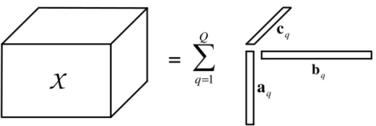
For anI1×I2×I3 third-order tensor X, its Q-component PARAFAC decom-position is given by:
xi1,i2,i3 =
Q
X
q=1 a(iq1)b
(q)
i2 c
(q)
i3 . (2)
The standard PARAFAC model for a three-way (3D) array expresses the orig-inal tensor as a sum of rank-one three-way factors, each one of which being an outer product of three vectors. Figure (1) illustrates the PARAFAC decompo-sition of tensor X. By analogy with the definition of matrix rank, the rank of a third-order tensor is defined as the minimum number of rank-one three-way components needed to decompose X [4].
The PARAFAC decomposition can also be represented in matrix notation. Define an I1 ×Q matrix A, I2 × Q matrix B and I3 ×Q matrix C with respective elements a(i1q) = [A]i1,q, b
(q)
i2 = [B]i2,q and c
(q)
i3 = [C]i3,q. Define also
a set of I2 ×I3 matrices Xi1··, i1 = 1,· · · , I1, a set of I3 ×I1 matrices X·i2·,
i2 = 1,· · · , I2 and a set ofI1×I2 matricesX··i3,i3 = 1,· · · , I3. Based on these
definitions, the model (2) can be written in three different ways:
Xi1··=
Q
X
q=1 a(i1q)b
(q)c(q)T
=BDi1(A)C
T
, i1 = 1,· · · , I1,
X·i2·=
Q
X
q=1 b(i2q)c
(q)a(q)T =CD
i2(B)A
T, i2 = 1,
· · · , I2,
X··i3=
Q
X
q=1 c(i3q)a
(q)b(q)T
=ADi3(C)B
T
, i3 = 1,· · · , I3,
where a(q), b(q) and c(q) are the q-th column of matrices A, B and C
re-spectively, and the operator Di1(A) forms a diagonal matrix with the i1-th
row of A. The matrices Xi1··, i1 = 1,· · · , I1, X·i2·, i2 = 1,· · · , I2, and X··i3,
i3 = 1,· · · , I3 can be interpreted as slices of the tensor along the first,
=
∑ = Q q 1 q a q b q cX
Fig. 1.Q-factor PARAFAC decomposition of a 3D tensor.
X··i3, i3 = 1,· · ·, I3 into a I3I1×I2 matrix, we get the unfolded matrixX1:
X1 =
X··1
...
X··I3 =
AD1(C) ...
ADi3(C)
BT = (C⋄A)BT (3)
Similarly, for the two other modes, we have:
X2 =
X·1·
...
X·I2· =
CD1(B) ...
CDI2(B)
AT = (B⋄C)AT, (4)
X3 =
X1··
...
XI1·· =
BD1(A) ...
BDI1(A)
CT = (A
⋄B)CT, (5)
whereX2 andX3are of dimensionsI2I3×I1 andI1I2×I3respectively.
Unique-ness of the PARAFAC decomposition was firstly studied in [6,19], and more recently in [20,21]. The first formal proof was provided by Kruskal [4]. This proof has been recently revisited and clarified in [21]. In [22], the uniqueness condition was extended to the complex case while [23] further generalized this condition to tensors of an arbitrary order.
2.2 PAFAFAC-based decomposition with constrained structure
Let X ∈ CI1×I2×I3
be a third-order tensor and define two sets of matrices
{A(1), . . . ,A(Q)} ∈ CI1×R1 and
{B(1), . . . ,B(Q)} ∈ CI2×R2 with typical
ele-ments a(i1q,r)1 = [A
(q)]
i1,r1, b
(q)
i2,r2 = [B
(q)]
i2,r2, and a set ofQ third-order tensors
{C(1), . . . ,C(Q)} ∈ CR1×R2×I3
de-composition in scalar form is given by:
xi1,i2,i3 =
Q
X
q=1
R1 X
r1=1
R2 X
r2=1
a(i1q,r)1b
(q)
i2,r2c
(q)
r1,r2,i3. (6)
This decomposition expresses the tensorxi1,i2,i3 as a sum ofQtrilinear blocks,
each one of them being given by the sum ofR1R2 triple products. Define a set
of Q matrices {C(1), . . . ,C(Q)} ∈CI3×R1R2 in the following way:
[C(q)]
i3,(r1−1)R2+r2 =c
(q)
r1,r2,i3, q= 1, . . . , Q,
where the matrix C(q) is linked to tensor C(q) by:
C(q) = [vec(C··(q1)T)· · ·vec(C (q)T
··I3 )]
T
,
C(··qi)3 ∈C
R1×R2 being thei3-th matrix slice of
C(q), i3 = 1, . . . , I3.
Let us define the block-matrices A = [A(1)· · ·A(Q)] ∈ CI1×QR1, B =
[B(1)· · ·B(Q)] ∈ CI2×QR2
and C = [C(1)· · ·C(Q)] ∈ CI3×QR1R2
, and block-diagonal constraint matrices Ψ = IQ ⊗ (IR1 ⊗ 1
T
R2) = IQ ⊗ Ψ and Φ = IQ⊗(1TR1 ⊗IR2) = IQ⊗Φ, of dimensions QR1 ×QR1R2 and QR2 ×QR1R2
respectively. By analogy with (3), (4) and (5), the unfolded matrices X1, X2
and X3 are given by:
X1= (C⋄AΨ)Φ
T
BT,
X2= (BΦ⋄C)Ψ
T
AT, (7)
X3= (AΨ⋄BΦ)CT.
The demonstration of (7) is provided in the Appendix, considering the un-folded matrix X3. By comparing (7) with (3)-(5), we deduce the following
correspondences: A → AΨ, B→ BΦ and C→ C. Therefore, X··i3 ∈ C
I1×I2
of X can be expressed as:
X··i3 =
Q
X
q=1
A(q)ΨDi3(C
(q))(B(q)Φ)T
. (8)
A more compact notation for (8) is the following:
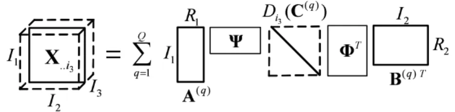
X··i3 =AΨDi3(C)(BΦ)
T
. (9)
An illustration of this decomposition is shown in Fig. 2.
✁
✂ ✄
☎ ✆ ✞ ✟
✠
✡ ☛
✆
✝
✟
☞
✌
✍
✌
✟
✆
✝
✎
✏
✂
✁
✑
=
✒
✓
✓✕✔
X ∑
=
✖
✟
✁
✁
✑
✏
✑
✁
✑
✏
✑
✗
✑
Fig. 2. Illustration of a PARAFAC decomposition with constrained structure.
(PARALlel profiles with LINear Dependencies), although the modeling ap-proach here is more general. The model proposed here, is a sort of “Block-PARAFAC” model composed ofQtensor blocks, where interactions involving factors of different modes are confined to each block. In [29] and [30], we pro-pose a more general formulation of this model, considering that the interaction pattern may differ from block to block. In the context of this work, allowing different interaction patterns per block is equivalent to assume users with different number of multipaths as well as with different multipath structure [30].
2.2.1 Uniqueness
Consider the set of matrix-slicesX··i3,i3 = 1, . . . , I3, given in (8). Assume that
the component matrices A(q) ∈ CI1×R1
, B(q) ∈ CI2×R2
and C(q) ∈ CI3×R1R2
are full-column rank. If every set {A(1), . . . ,A(Q)}, {B(1), . . . ,B(Q)} and {C(1), . . . ,C(Q)} is linear independent, a necessary condition for the
sepa-ration/resolution of the Qblocks is:
min
µ
⌊R1R2I1I2 ⌋,⌊I1I3 R2 ⌋,⌊
I2I3 R1 ⌋
¶
≥Q, (10)
where ⌊·⌋ stands for the greatest integer number that is smaller than its argument. In this case, there are non-singular block-diagonal matrices Ta
∈ CR1Q×R1Q
, Tb ∈ CR2Q×R2Q and Tc ∈ CR1R2Q×R1R2Q, with diagonal blocks
T(q)
a ,T
(q)
b and T(cq) satisfying
(T(q)
a ⊗T
(q)
b )
−1
=T(q)T
c , q= 1, . . . , Q,
so that
c
A=A(Π⊗IR1)Ta, Bb =B(Π⊗IR2)Tb, Cb =C(Π⊗IR1R2)Tc (11)
give rise to the same X··i3, i3 = 1, . . . , I3, where Π ∈ C
Q×Q is a
block-permutation matrix. Permutation of theR1 columns of A(q), the R2 columns
of B(q) and R
1R2 columns of C(q), q = 1, . . . , Q, are considered unimportant
✘
θ
✙
θ
✚
θ ∆
1
✛
a
n
te
n
n
a
a
rr
a
y
✜
θ
∆
✢
✣
Cluster 1
Cluster L
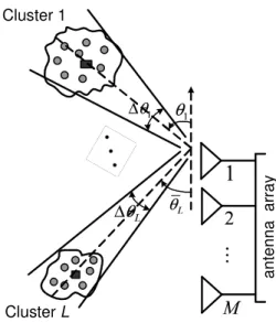
Fig. 3. Schematic representation of the multipath propagation scenario.
3 Channel and System Models
Let us consider a linear and uniformly-spaced array ofM antennas receiving signals from Q co-channel users. Assume that the signal transmitted by each user is subject to multipath propagation and arrives at the receiver via L
effective specular paths1. The propagation channel is assumed to be
time-dispersive and it is considered that multipath delay spread exceeds the inverse of the coherence bandwidth of the system, so that fading is frequency-selective. Following [24–26], we assume that there areLsignificant scatterer clusters (see Fig. 3) and that each of the multipaths emanating from the same scatterer cluster has the same delay. Each clustered multipath has a mean angle of arrival θl and an angle spread ∆θl. The adopted model is valid in practice,
provided that the receive antenna array, generally located in a base transceiver station, is sufficiently high so that it is unobstructed and no local scattering occurs. These assumptions on the propagation scenario are typical for cellular suburban deployments [27], where the base transceiver station is on a tower or on the roof of a building.
The channel impulse response is assumed to span K symbols. The discrete-time base-band representation of the signal received at them-th antenna of a linear and uniformly-spaced array at the n-th symbol interval is given by:
xm(n) = Q
X
q=1
L
X
l=1
βl(q)am(θlq) K
X
k=1
g(k−1−τlq)s(q)(n−k+ 1) +vm(n),
where βl(q) is the fading envelope of the l-th path of the q-th user. The term
1 In this model we have assumed that all users have the same number of multipaths
am(θlq) is the response of the m-th antenna to the l-th path of the q-th user,
θlq being the associated angle of arrival. Similarly, the term τlq is the
propa-gation delay (normalized by the symbol periodT) and the term g(k−1−τlq)
represents thek-th component of the pulse-shaping filter response. The chan-nel impulse response has finite duration and is assumed to be zero outside the interval [0,(K −1)T). Finally, s(q)(n) is the symbol transmitted by the q-th user at the n-th symbol interval and vm(n) is the measurement noise at
them-th antenna at then-th symbol interval. The received signal vectorx(n)
∈CM is given by:
x(n) =
Q
X
q=1
L
X
l=1 βl(q)a
(q)
l g
(q)T l s(
q)(n) +v(n),
where
a(lq)= [a1(θlq)· · ·aM(θlq)]T ∈CM
g(lq) = [g(−τlq)· · ·g(K −1−τlq)]T ∈RK
s(q)(n) = [s(q)(n)· · ·s(q)(n−K+ 1)]T ∈CK,
are the array steering vector, the pulse-shaping filter response vector and a symbol vector respectively, with q = 1, . . . , Q and l = 1, . . . , L. For the q-th user, let us define:
A(q) = [a(1q)· · ·a (q)
L ]∈C M×L
b(q) = [β(q) 1 · · ·β
(q)
L ] T
∈CL×1
G(q) = [g(q) 1 · · ·g
(q)
L ]T ∈RL×K
H(q)=Diag(b(q))G(q)
∈CL×K
S(q) = [s(q)(1)· · ·s(q)(N)]T ∈CN×K,
where A(q),b(q) and G(q) assemble L array responses, path gains and pulse
shape responses respectively. H(q) is the overall temporal channel response
matrix associated with the q-th user, i.e. the pulse-shaping filter response matrix scaled by the multipath gains andS(q)is Toeplitz, with the first row and
column defined ass(q)
row = [s(q)(1) 0 · · ·0] ands
(q)
col = [s(q)(1)s(q)(2) · · · s(q)(N)]T
respectively.
Assuming that the wireless channel is invariant during N consecutive symbol intervals, the received signal can be expressed as a matrix X ∈ CM×N that
can be decomposed in the following form:
X= [x(1)· · ·x(N)] =
Q
X
q=1
Now, defining:
A= [A(1)· · ·A(Q)]∈CM×QL
B=Diag([b(1)T · · ·b(Q)T])∈CQL×QL
G=BlockDiag(G(1)· · ·G(Q))
∈RQL×QK
S= [S(1)· · ·S(Q)]
∈CN×QK,
the received signal matrix (12) can be rewritten in a more compact block-matrix form as:
X=AHS+V, (13)
with H=BG ∈CQL×QK.
Model (13) serves as a reference model for the development of the new 3D PARAFAC-based model unifying the received signal model of temporally-oversampled, DS/CDMA and OFDM systems. In other words, the basicspace
andtime dimensions of the received signal (13) that are represented by matri-ces A and S, will be similarly defined when considering the proposed tensor model, the main difference being in the incorporation of a third dimension to the received signal as a consequence of oversampling, spreading or multicarrier modulation.
4 Tensor Modeling of the Received Signal
The key step to obtain a 3D PARAFAC model is linked to an appropriate definition of theoverall channel response matrixHfor each considered system. Thus, in the same way that A and S model the space and time dimensions of the 2D received signal model (13), H models the third dimension for the proposed 3D tensor model. This additional dimension can be anoversampling
dimension, a spreading dimension or afrequency dimension depending on the considered system. In the following, we define the concept of overall channel response for each one of the considered systems. Then, the tensor notation is introduced to model the received signal of each system as a 3D PARAFAC-based tensor model.
4.1 Temporally-Oversampled System
At the output of each receiver antenna, the signal is sampled at a rate that is
in the temporal resolution can be interpreted as an incorporation of a third axis (or dimension) to the received signal, called theoversampling dimension. We define the p-th oversample associated with the k-th component of the pulse-shaping filter response to the (l, q)-th path as the following third-order tensor:
gl,k,p(q) =g(k−1 + (p−1)/P −τlq), p= 1, . . . , P.
The overall channel response, array response and symbols are defined as:
h(l,k,pq) =βl(q)gl,k,p(q) , a(m,lq) =am(θlq), s( q)
n,k =sq(n−k+ 1).
The received signal can be interpreted as a 3D tensor X ∈ CM×N×P. Its
(m, n, p)-th scalar component can be decomposed as:
xm,n,p = Q
X
q=1
L
X
l=1 a(m,lq)
K
X
k=1
h(l,k,pq) s(n,kq) +vm,n,p. (14)
By comparing with (6), we have the following correspondences:
(I1, I2, I3, R1, R2,A,B,C)→(M, N, P, L, K,A,S,H) (15)
Equation (14) is thescalar notation for the received signal tensor. It expresses the received signal in the form of summations and products involving three factors a(m,lq), hl,k,p(q) and s(n,kq) associated with space, oversampling and time di-mensions of the received signal, respectively. (14) can be alternatively written in matrix-slice form. Let us define a pulse-shape response matrixG(lq) ∈RP×K
as:
Gl(q) = [g(l,q1)gl,(q2) · · ·g(l,Kq)],
where g(l,kq) = [g
(q)
l,k,1g (q)
l,k,2· · ·g (q)
l,k,p]T ∈ RP collects the P oversamples associated
with the k-th component of the (l, q)-th pulse-shape response. Define also
G(q) = [G(q) 1 · · ·G
(q)
L ] ∈ RP×LK as a matrix concatenating the L pulse-shape
response vectors associated with the q-th user. The overall temporal channel response matrix H(q) can be expressed as:
H(q) =G(q)(Diag(b(q))⊗IK) ∈CP×LK. (16)
Fixing the oversampling dimension, and using the analogy with (8) and the correspondences (15), the space-time sliceX. . p∈CM×N,p= 1, . . . , P, can be
factored as:
X. . p= Q
X
q=1
A(q)ΨDp(H(q))(S(q)Φ)T +V. . p, p= 1, . . . , P, (17)
whereΨ=IL⊗1TK andΦ=1TL⊗IK are the constraint matrices of the tensor
4.2 DS/CDMA System
At the transmitter, each symbol is spread by a signature (spreading code) sequence of length J with period Tc = T /J, where T is the symbol period.
The spreading sequence associated with the q-th user is denoted by c(q) =
[c(1q)c(2q)· · ·c(Jq)]T ∈CJ. As a result of spreading operation, each symbol to be
transmitted is converted intoJ chips. The chip-sampled pulse-shape response to the (l, q)-th path is defined in scalar form as:
gl,k,j(q) =g(k−1 + (j−1)/J −τlq), j = 1, . . . , J.
A scalar component of the overall channel response, i.e. including path gains, is defined as h(l,k,jq) =βl(q)g(l,k,jq) . The received signal can be interpreted as a 3D tensor X ∈ CM×N×J and its (m, n, j)-th scalar component has the following
factorization:
xm,n,j = Q
X
q=1
L
X
l=1 a(m,lq)
K
X
k=1
J
X
j′=1
h(l,k,jq) −j′c
(q)
j′ s
(q)
n,k+vm,n,j. (18)
Equation (18) decomposes the received signal in the form of summations and products involving four scalar factors a(m,lq), h
(q)
j,l,k,c
(q)
j and s
(q)
n,k. Defining
u(l,k,jq) = J
X
j′=1
h(l,k,jq) −j′c
(q)
j′
as the convolution between the spreading sequence and the overall channel response, we can rewrite (18) as:
xm,n,j = Q
X
q=1
L
X
l=1 a(m,lq)
K
X
k=1
u(l,k,jq) s
(q)
n,k+vm,n,j. (19)
Note that (19) is equivalent to (14), where u(l,k,jq) plays the role of h
(q)
l,k,p and
J →P. Therefore, by fixing the spreading dimension and slicing the received signal tensor X ∈ CM×N×J along the third-dimension, its j-th slice X
. . j ∈
CM×N, j = 1, . . . , J, is given by:
X. . j = Q
X
q=1
A(q)ΨDj(U(q))(S(q)Φ)T +V. . j, j = 1, . . . , J, (20)
where U(q) is defined as:
U(q) =C(q)H(q)
C(q) ∈ CJ×J being a Toeplitz matrix with first row and column defined as
c(q)
row = [c(q)(1) 0 · · · 0] and c
(q)
col = [c(q)(1)c(q)(2) · · · c(q)(J)]T respectively, and
H(q) being analogous to that defined in (16), where J replacesP.
4.3 OFDM System
In an OFDM system, the symbol sequence to be transmitted is organized into blocks of F symbols (serial-to-parallel conversion). Multicarrier modulation consists in linearly combining the F symbols using an inverse N ×N Fast Fourier Transform (IFFT) matrix. After the IFFT stage, a cyclic prefix (CP) of lengthK is inserted to each OFDM block 2, before transmission. Due to the insertion of CP, the resulting OFDM block has lengthF +K. At the receiver inverse processing is done. The CP is removed and each received OFDM block is linearly combined using an N ×N Fast Fourier Transform (FFT) matrix. Thanks to the use of IFFT/FFT together with insertion/removal of the CP, it can be shown [17] that the length-K convolutive channel is converted into a set of F scalar channels, i.e. the overall channel at each subcarrier is frequency-flat. This means that the overall channel matrix has a diagonal frequency response.
Let us define h(l,fq) = βl(q)g(l,fq) as a scalar component of the overall frequency channel response at the f-th subcarrier, associated with the (l, q)-th path. The scalar s(n,fq) denotes the f-th symbol of the n-th OFDM block associated with theq-th user. The received signal is also a 3D tensor and its (m, n, f)-th scalar component can be decomposed as:
xm,n,f = Q
X
q=1
L
X
l=1
a(m,lq) h(l,fq)s(n,fq) +vm,n,f. (22)
As it has been done for the previous systems, we are interested in representing the received signal tensor in matrix- slice notation. Let us define the vector
s(q)
n = [s
(q) 1,ns
(q) 2,n · · · s
(q)
F,n]T ∈CF collecting the symbols associated with then-th
OFDM block, n = 1, . . . , N. We define ˘Gl(q) ∈ RF×F as a circulant channel
matrix built up from the (l, q)-th pulse-shape responseg(lq) = [gl,(q1)gl,(q2)· · ·gl,K(q)]T
∈RK. Let
Ωcp =
0K×(F−K) IK
IF
, Ωcp= [0F×K IF],
be the matrices that represent the insertion and removal of the CP, of dimen-sions (F+K)×F andF×(F+K) respectively, and define a (F+K)×(F+K)
2 The CP is used to avoid interference between adjacent OFDM blocks. Its length
Toeplitz matrix ˜G(lq) = T oeplitz[g
(q)
l ]. The (l, q)-th circulant matrix ˘G
(q)
l is
given by:
˘
G(lq)= ΩcpG˜
(q)
l Ωcp.
Note that the circulant structure of ˘G(lq) ∈ CF×F is an equivalent
represen-tation of the convolution matrix ˜G(lq), when it is pre- and post-multiplied by
the matrices that represent the removal and insertion of the CP, respectively. For further details on this construction, please see [17].
Define ˘G(q) = [ ˘G(q) 1 · · ·G˘
(q)
L ] ∈RF×LF as a block-circulant matrix
concatenat-ing theLcirculant channel matrices associated with theq-th user. By analogy with (16), the overall circulant channel matrix H˘(q) can be written as:
˘
H(q)= ˘G(q)³Diag(b(q)) ⊗IF
´
∈CF×LF.
Taking IFFT/FFT transformations at the transmitter/receiver into account, the q-th user overall frequency response channel matrix Λ(q) = [Λ(q)
1 · · ·Λ (q)
L ]
∈CF×LF, can be expressed as:
Λ(q) =ΓH˘(q)(I
L⊗Γ)H, (23)
where Γ ∈ CF×F is a FFT matrix the (i, k)-th entry of which is given by
γi,k = (1/
√
F)·exp(−j2πik/N), i, k = 0,1, . . . , N −1. Note that Λ(lq) is a
diagonal matrix holding the vectorh(lq) = [h(1q,l)h2(q,l) · · ·h(F,lq)]T, on its diagonal,
l= 1, . . . , L, i.e., Λ(lq) =Diag(h
(q)
l ).
Now, collect N symbol blocks in S(q) = [s(q) 1 · · ·s
(q)
N ] ∈ CF×N. Taking these
definitions into account, the f-th slice X. . f ∈ CM×N, f = 1, . . . , F, of the
received signal tensor X ∈CM×N×F can be decomposed as:
X. . f = Q
X
q=1
A(q)ΨD
f(Λ(q))(S(q)Φ)T +V. . f, f = 1, . . . , F. (24)
5 Unified PARAFAC model
In this section we formalize the unified PARAFAC model for the temporally-oversampled, DS/CDMA and OFDM systems. The proposed PARAFAC model brings together the tensor modeling of the received signal for these systems in a single model using a unified mathematical notation. The pro-posal of a unique model is based on the observation that the received signal for the three considered systems can be formulated as 3D tensors following fundamentally the same PARAFAC decomposition.
For convenience, we rewrite the scalar representations for the received signal given by (14), (19) and (22) for the temporally-oversampled, DS/CDMA and OFDM systems respectively, in the following way:
xm,n,p= Q
X
q=1
L
X
l=1
K
X
k=1 a(m,lq) s
(q)
n,kh
(q)
l,k,p+vm,n,p,
xm,n,j= Q
X
q=1
L
X
l=1
K
X
k=1
a(m,lq) s(n,kq)u(l,k,jq) +vm,n,j, u( q)
l,k,p =h
(q)
l,k,j ∗c
(q)
j , (25)
xm,n,f= Q
X
q=1
L
X
l=1
F
X
f′=1
a(m,lq) s
(q)
n,f′h
(q)
l,f′,f+vm,n,f, h
(q)
l,f′,f =h
(q)
l,fδf′f.
The three tensor models are quite similar. Note that the basic difference is on the definition of the term associated with the third-dimension of the equivalent PARAFAC model, which ish(l,k,pq) for oversampled case,u
(q)
l,k,j for the DS/CDMA
case and h(l,fq)′,f for the OFDM case. Another difference is on the structure of
the component matrix S(q), which is not Toeplitz in the OFDM model.
In order to link the unified tensor model to (6), we defineI3as the length of the third dimension of the received signal tensor. For the temporally-oversampled system (I3, R2) = (P, K), for the DS/CDMA system (I3, R2) = (J, K) and for the OFDM system (I3, R2) = (F, F). The other parameters, which are common for all the systems are I1 = M, I2 = N, R1 = L. In its general
form, the tensor modeling of the three systems can be unified in the following expression:
X. . i3 =
Q
X
q=1
A(q)ΨD
i3(W
(q))(S(q)Φ)T +V
. . i3, i3 = 1,· · ·, I3,
where
Ψ=IL⊗1TR2 ∈C
L×LR2
, Φ=1T
L⊗IR2 ∈C
LR2×R2
,
and W(q) is either H(q) (c.f. (16)), or U(q) (c.f. (21)) or Λ(q) (c.f. (23)),
Finally, concatenatingI3 space-time slices X. . i3, i3 = 1, . . . , I3 and using (7),
we get:
X1 = (W⋄AΨ)(SΦ)T, (26)
whereΨ=IQ⊗ΨandΦ=IQ⊗Φ. The factorization ofX2 = [XT.1.· · ·XT. N .]T
∈CI3N×M and X
3 = [XT1. .· · ·XM . .T ]T ∈CN M×I3 follows (4) and (5).
Compar-ing (26) and (7) we deduce the followCompar-ing correspondences: A → A, B → ST
and C → W. The link of the general PARAFAC model (7) to the tensor model of each considered system is provided in Table 1 for comparison.
Oversampled DS/CDMA OFDM
(I3) oversampling(P) spreading(J) frequency(F)
(R2) delay(K) delay(K) frequency(F)
W H= [H(1)· · ·H(Q)] U= [U(1)· · ·U(Q)] Λ= [Λ(1)· · ·Λ(Q)]
dimensions P ×QLK J ×QLK F ×QLF
structure no structure no structure diagonal blocks MatrixS S= [S(1)T · · ·S(Q)T]T S= [S(1)T · · ·S(Q)T]T S= [S(1)T · · ·S(Q)T]T
dimensions QK ×N QK×N QF ×N
structure block-Toeplitz block-Toeplitz no structure
Table 1. Link of the PARAFAC model for each communication system
6 Application to Blind Multiuser Equalization
The blind multiuser equalization problem consists in recovering the informa-tion sequence from several users under the assumpinforma-tion of frequency-selective fading. In other words, a blind multiuser equalizer performs the tasks of signal separation and equalization. In this paper, we propose a PARAFAC-based receiver performing user separation and equalization iteratively. For the temporally-oversampled system, multiuser signal separation is carried out in the 3D tensor space, exploiting oversampling, time and space dimensions of the received signal.
component matrices from which the PARAFAC model parameters can be de-termined. In turn, the goal of the subspace+FA stage is to solve the partial rotation ambiguity problem that is inherent to the proposed model as well as to estimate the transmitted symbols in the 2D space, exploiting the FA prop-erty. The FA-projected symbols are in turn used as an input to the PARAFAC stage to refine the multiuser signal separation in the 3D space. In the following, we describe the proposed algorithm.
6.1 Iterative PARAFAC-Subspace Receiver
For the received signal tensor X (M×N ×P), multiuser signal separation is carried out in the 3D tensor space using the ALS algorithm, which consists in estimating in an alternating way three matrices Zb1 ∈ CN×KQ, Zb2 ∈ CM×LQ
and Zb3 ∈ CP×KLQ from the matrix representations Xi=1,2,3 of the received
signal tensor. The multiuser signal separation problem is formulated as a set of three independent nonlinear least squares problems:
b
Z1=argmin
Z1
kX1−(Z3⋄Z2Ψ)(Z1Φ)Tk2F,
b
Z2=argmin
Z2
kX2−(Z1Φ⋄Z3)(Z2Ψ)Tk2F, (27)
b
Z3=argmin
Z3
kX3−(Z2Ψ⋄Z1Φ)ZT3k2F.
Thus, one iteration of the multiuser signal separation stage has three steps. At each step one component matrix is updated while the others are fixed to the values obtained at the previous step. By analogy with (26), we have Z1 →S,
Z2 →AandZ3 →W. Uniqueness ofAandWis not important in the present
context since we are interested in recovering the user symbol sequences (which is the final goal in the blind multiuser equalization problem) that should be extracted fromS. From (11), and ignoring the trivial permutation ambiguity, we have:
b
S(1) =T(1)S(1) , . . . , Sb(Q) =T(Q)S(Q),
where T(q), q = 1, . . . , Q are non-singular (ambiguity) matrices to be
de-termined. The determination of T(q) and Sb(q) can be viewed as an
equiva-lent single-input multiple-output (SIMO) blind channel identification prob-lem, whereT(q),q = 1, . . . , Qplay the role of virtual length-K SIMO channels
withK outputs. The subspace+FA stage of the proposed receiver aims at de-termining T(q), q = 1, . . . , Q, by the following steps. Matrices Tb(1),· · · ,Tb(Q)
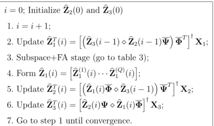
i= 0; Initialize Zb2(0) and Zb3(0)
1.i=i+ 1; 2. Update ZbT
1(i) =
h³ b
Z3(i−1)⋄Zb2(i−1)Ψ
´
ΦTi†X1;
3. Subspace+FA stage (go to table 3); 4. FormZb1(i) =
h b
Z(1)1 (i)· · ·Zb (Q) 1 (i)
i
; 5. Update ZbT
2(i) =
h³ b
Z1(i)Φ⋄Zb3(i−1)
´
ΨTi†X2;
6. Update ZbT
3(i) =
h b
Z2(i)Ψ⋄Zb1(i)Φ
i†
X3;
7. Go to step 1 until convergence.
Table 2. Pseudo-code for the iterative PARAFAC-Subspace algorithm
for q = 1 toQ, – PartitionZb1(i) =
h b
Z1(1)(i)· · ·Zb1(Q)(i)i; – Determine T(q)(i) from Zb(q)
1 (i) (subspace method);
– Sb(q)(i) = [Tb(q)(i)]−1Zb(q) 1 (i);
– bs(q)(i) =Average over the columns of Sb(q)(i);
– es(q)(i) =Proj[bs(q)(i)];
– Zb(1q)(i) = Toeplitz [es(q)(i)];
endq
Table 3. Pseudo-code for the subspace + FA projection stage
can be estimated (up to permutation) by pseudo-inversion. An estimation of user symbol sequences bs(q) ∈ CN is obtained by properly averaging over the
columns of Sb(q) followed by a FA-projection. We assume that the first symbol
of each user sequence is known and equal to 1. This allows us to eliminate scaling ambiguity by normalizing each estimated symbol sequence es(q)(i) by
its first element. An updated (post-equalized) version of Zb1 is then formed
and used as an input to the PARAFAC stage to refine user signal separation in the 3D space. At the end of the algorithm, the permutation ambiguity is resolved using a greedy least squares (S(q),Sb(q))-column matching algorithm
[11].
received signal tensor can be obtained from the following equation:
ei =
° °
°X1−
³ b
Z3(i)⋄Zb2(i)Ψ
´
(Zb1(i)Φ)T
° °
°F. (28)
We declare convergence at thei-th iteration when |ei−ei−1| ≤10−5.
7 Simulation results
In this section, the performance of the proposed PARAFAC-based blind mul-tiuser receiver is evaluated through computer simulations. Each obtained re-sult is an average overR= 1000 independent Monte Carlo runs. For each run, multipath fading gains are generated from an i.i.d. Rayleigh generator while the user symbols are generated from an i.i.d. distribution and are modulated using binary-phase shift keying (BPSK). Perfect synchronization is assumed at the receiver. In all cases, a block of N = 100 received samples is used in the blind estimation process. The channel impulse response follows a raised cosine pulse shape with roll-off factor 0.35. We consider K = 2 channel taps,
Q = 2 users and a fixed oversampling factor P = 8. At the beginning of the algorithm Zb(0)2 and Zb
(0)
3 are randomly initialized. More sophisticated
initial-ization strategies exist, which are based on Tucker3 compression [11] or on eigenanalysis [12], but they are beyond the scope of this work. We have ob-served however that convergence of the estimates is rapidly achieved (within 10 ALS iterations in most of cases), and this is attributed to the use of the FA property within the ALS loops.
7.1 BER calculation
We adopt the following criterion for the Bit-Error-Rate (BER) calculation. 1% of the total number of runs are discarded, corresponding to inevitable bad runs that reach a local minimum. The criterion for selecting the bad runs is based on the observation of the steady state estimation error, i.e., the error between the received tensor and the tensor constructed from estimated components matrices after convergence. The runs with the highest non-convergent error values are discarded from the BER averaging process. For the bit-error-rate (BER)versus signal-to-noise ratio (SNR) results, the BER shown is the BER averaged over both users and R independent runs, i.e.:
BER = 1
R
R
X
r=1
BER1(r) + BER2(r)
2 ,
0 2 4 6 8 10 12 14 16 18 20 10−4
10−3 10−2 10−1 100 101
Number of Iterations
Normalized estimation error
SNR=5
SNR=10
SNR=15
SNR=20
SNR=25
SNR=30
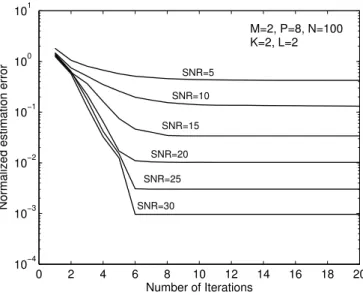
M=2, P=8, N=100 K=2, L=2
Fig. 4. Convergence of the PARAFAC-Subspace receiver. First propagation scenario.
7.2 Propagation scenarios
We adopt the multipath propagation model described in Section 3 and consider
L= 2 effective multipaths per user, each path being associated with a different cluster of scatterers. Cluster angle spreads are the same for both users and are given by (∆θ1q,∆θ2q) = (0◦,5◦), q = 1,2. Concerning the mean angle
of arrival, we consider two propagation scenarios. In the first one, we have (θ11, θ21) = (0◦,20◦) for the first user and (θ12, θ22) = (−10◦,10◦) for the
second one. The second propagation scenario is more challenging. The mean angle of arrival of the first (zero-delayed) path of both users is identical, and we have θ11 = θ12 = 0◦, while the other multipaths have the same angles as
those of the first scenario. Unless otherwise stated, all multipaths have the same average power E[βlqβlq∗] = 1, l = 1, . . . , L, q = 1, . . . , Q.
7.3 Performance results
We begin by evaluating the convergence of the proposed PARAFAC-Subspace algorithm. Figure 4 shows typical convergence curves, considering the first propagation scenario. The median values of the normalized errore2
i/(M P N),
where ei is given in 28, are plotted as a function of the iterations for various
SNR values. It can be seen from Fig. 4 that the algorithm rapidly converges, usually within 10 iterations. We have observed that convergence is actually accelerated due to the use of FA property within the ALS loops.
0 5 10 15 20 25 30 35 10−5
10−4 10−3 10−2 10−1
SNR (dB)
BER
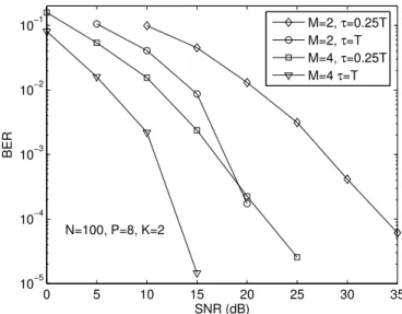
M=2, τ=0.25T M=2, τ=T M=4, τ=0.25T M=4 τ=T
N=100, P=8, K=2
Fig. 5. BER versus SNR results. First propagation scenario.
the multipath delay spread, we consider two cases. In the first one (τ1q, τ2q) =
(0, τ) = (0, T), while in the second one (τ1q, τ2q) = (0, τ) = (0,0.25T),q = 1,2.
The results are shown in Figure 5, for M = 2 and 4 receive antennas. It can be seen that the BER performance of the proposed receiver is remarkable, even withM = 2 receive antennas. A significant performance gain is observed when the number of receive antennas is increased from 2 to 4, since more degrees of freedom are available in the space domain to separate the two user signals. Improved performance is obtained when τ = T, i.e., when the delay of the second multipath (for both users) coincides with one symbol period. Multipath combination is more effective when τ = T, since the multipaths are better distinguished in the time domain. Moreover, whenτ = 0.25T, some multipath energy is spread beyond K = 2 symbol periods and this is ignored in our tensor model.
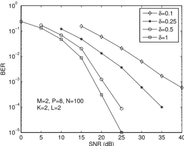
We now consider the second propagation scenario, where the first path of both users have identical angles of arrival. We want to illustrate that in this type of scenario, path diversity becomes important and frequency-selectivity indeed helps the separability of the user signals in the time domain. In order to evaluate this, the average power of the second (one-symbol delayed) path of each user is varied. We define δ as the average ratio between the gain of the second and first multipaths, which are assumed equal for both users. We considerδ= 0.1,0.25,0.5 and 1. According to Figure 6, improved performance is obtained when the first and second paths have the same average power, i.e.,
0 5 10 15 20 25 30 35 40 10−5
10−4 10−3 10−2 10−1 100
SNR (dB)
BER
δ=0.1
δ=0.25
δ=0.5
δ=1
M=2, P=8, N=100 K=2, L=2
Fig. 6. BER versus SNR results. Second propagation scenario.
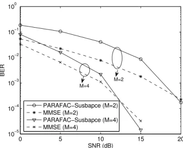
In order to provide a performance reference for the proposed PARAFAC-Subspace receiver, we also evaluate the performance of the Minimum Mean Square Error (MMSE) receiver. In contrast to our blind iterative PARAFAC-Subspace receiver, the MMSE one assumes perfect knowledge of all channel parameters as well as the knowledge of the SNR. We consider M = 2 and 4 receive antennas. Figure 7 shows that the PARAFAC-Subspace receiver has nearly the same BER vs. SNR improvement than that of MMSE with perfect channel knowledge. The gap between both receivers is smaller forM = 4. For example, considering a target BER of 10−2, the proposed receiver provides a
loss in performance of 5dB forM = 2 and 3dB forM = 4, with respect to the MMSE receiver.
8 Conclusions and Perspectives
0 5 10 15 20 10−5
10−4 10−3 10−2 10−1 100
SNR (dB)
BER
PARAFAC−Susbapce (M=2) MMSE (M=2)
PARAFAC−Susbapce (M=4) MMSE (M=4)
M=2 M=4
Fig. 7. Blind PARAFAC-Subspace receiver versus MMSE receiver with perfect chan-nel knowledge.
blind multiuser equalization. The proposed algorithm combines PARAFAC and a subspace method together with the use of the FA property in order to perform user signal separation and equalization iteratively. According to our simulation results, the performance of the iterative PARAFAC-Subspace is remarkable and not so far from the MMSE solution with perfect knowledge of propagation parameters.
Appendix
Here, we provide a demonstration of (7). This is done by expanding the tensor
xi1,i2,i3 in (6) using Kronecker products of canonical vectors [32]:
xi1,i2,i3 =
Q
X
q=1
R1 X
r1=1
R2 X
r2=1
a(i1q,r)1b
(q)
i2,r2c
(q)
r1,r2,i3. (29)
Consider the canonical bases E(I1) =
{e(I1)
1 ,e (I1)
2 , . . . ,e (I1)
I1 }, E
(I2) =
{e(I2)
1 ,e (I2)
2 , . . . ,e (I2)
I2 }and E
(I3)
={e(I3)
1 ,e (I3)
2 , . . . ,e (I3)
I3 }associated with vector
spacesRI1
,RI2
,RI3
, respectively. The unfolded matrix X3 ∈CI1I2×I3, defined
as xi1,i2,i3 = [X3](i1−1)I2+i2,i3, can be expanded in terms of these canonical
vectors in the following manner:
X3 =
I1 X
i1=1
I2 X
i2=1
I3 X
i3=1
xi1,i2,i3(e
(I1)
i1 ⊗e
(I2)
i2 )e
(I3)T
i3 . (30)
Substituting (29) into (30) we have:
X3=
I1 X
i1=1
I2 X
i2=1
I3 X
i3=1
Q
X
q=1
R1 X
r1=1
R2 X
r2=1
a(i1q),r1b
(q)
i2,r2c
(q)
r1,r2,i3(e
(I1)
i1 ⊗e
(I2)
i2 )e
(I3)T
i3 = Q X q=1 R1 X
r1=1
R2 X
r2=1
I1 X
i1=1 e(I1)
i1 a
(q)
i1,r1 ⊗ I2 X
i2=1 e(I2)
i2 b
(q)
i2,r2 I3 X
i3=1 e(I3)
i3 c
(q)
r1,r2,i3
T
.
Define a(q)
r1 as the r1-th column of A
(q) ∈ CI1×R1, b(q)
r2 as the r2-th column of B(q) ∈CI2×R2 andc(q)
r1,r2 as the [(r1−1)R2+r2]-th column ofC
(q) ∈CI3×R1R2,
and observe that:
I1 X
i1=1 e(I1)
i1 a
(q)
i1,r1 =a
(q)
r1 ,
I2 X
i2=1 e(I2)
i2 b
(q)
i2,r2 =b
(q)
r2 ,
I3 X
i3=1 e(I3)
i3 c
(q)
r1,r2,i3 =c
(q)
r1,r2,
we have:
X3 =
Q
X
q=1
R1 X
r1=1
R2 X
r2=1
(a(q)
r1 ⊗b
(q)
r2 )c
(q)T
r1,r2. (31)
Define the set of canonical vectors e(R2)
r2 , r2 = 1, . . . , R2. Inserting
(e(R2)
r2 )
Te(R2)
r2 = 1 into (31) gives:
X3 =
Q
X
q=1
R1 X
r1=1
R2 X
r2=1 h
(a(q)
r1 ⊗b
(q)
r2 )e
(R2)T
r2 i h
e(R2)
r2 c
(q)T r1,r2
i
. (32)
Considering the following property:
(a⊗b)cT =a1T nc⋄bc
with a∈Cna
,b ∈Cnb
, c ∈Cnc
and 1nc ∈C
nc
, we can rewrite (32) as:
X3=
Q
X
q=1
R1 X
r1=1
R2 X
r2=1 h
a(rq1)1
T R2 ⋄b
(q)
r2 e
(R2)T
r2 i h
e(R2)
r2 c
(q)T r1,r2
i = Q X q=1 R1 X
r1=1
R2 X
r2=1 R2 X i=1 ³ a(rq1)e
(R2)T
i ⋄b( q)
r2 e
(R2)T
r2
´
he(R2)
r2 c
(q)T r1,r2
i
. (33)
Since the summation overi= 1, . . . , R2 in brackets is null for everyi6=r2, we can rewrite (33) as:
X3 =
Q
X
q=1
R1 X
r1=1
R2 X
r2=1 h
a(q)
r1 e
(R2)T
r2 ⋄b
(q)
r2 e
(R2)T
r2 i h
e(R2)
r2 c
(q)T r1,r2
i
. (34)
Due to the presence of the unit vectore(R2)
r2 , we can rewrite (34) as:
X3=
Q
X
q=1
R1 X
r1=1
R2 X
r2=1 a(rq1)e
(R2)T
r2 ⋄
R2 X
r2=1 b(rq2)e
(R2)T
r2 R2 X
r2=1 e(R2)
r2 c
(q)T r1,r2
= Q X q=1 R1 X
r1=1 h
(a(q)
r1 ⊗1
T R2)⋄B
(q)iC(q)T
r1 , (35)
with C(q)
r1 =
R2 P
r2=1 c(q)
r1,r2e
(R2)T
r2 ∈C
I3×R2.
Now, consider the set of canonical vectors e(R1)
r1 , r1 = 1, . . . , R1. Inserting e(R1)T
r1 e
(R1)
r1 = 1 into (35) and using property (1), it follows that:
X3=
Q
X
q=1
R1 X
r1=1 e(R1)T
r1 e
(R1)
r1 ⊗ h
(a(rq1)⊗1
T R2)⋄B
(q)iC(q)T r1 = Q X q=1 R1 X
r1=1 h
e(R1)T
r1 ⊗ h
(a(q)
r1 ⊗1
T R2)⋄B
(q)ii
·he(R1)
r1 ⊗C
(q)T r1
i
. (36)
Note that:
e(R1)T
r1 ⊗ h
(a(q)
r1 ⊗1
T R2)⋄B
(q)i=he(R1)T
r1 ⊗(a
(q)
r1 ⊗1
T R2)
i
⋄he(R1)T
r1 ⊗B
(q)i,
which allows us to express (36) in the following form:
X3 =
Q
X
q=1
R1 X
r1=1 hh
e(R1)T
r1 ⊗(a
(q)
r1 ⊗1
T R2)
i
⋄he(R1)T
r1 ⊗B
(q)ii ·he(R1)
r1 ⊗C
(q)T r1
i
Due to the block structure with zeros introduced by the factor e(R1)
r1 , we can
rewrite (37) as:
X3 =
Q X q=1 R1 X
r1=1 e(R1)T
r1 ⊗(a
(q)
r1 ⊗1
T R2)
⋄ R1 X
r1=1 e(R1)T
r1 ⊗B
(q)
· R1 X
r1=1 e(R1)
r1 ⊗C
(q)T r1
(38) which leads to:
X3 =
Q
X
q=1
h
(A(q)⊗1TR2)⋄(1
T R1 ⊗B
(q))i
·C(q)T. (39)
Now, using the property (1) of the Kronecker product, we have:
A(q)⊗1TR2 = (A
(q)
⊗1)(IR1 ⊗1
T
R2) = A
(q)(I
R1 ⊗1
T R2
| {z }
Ψ
) = A(q)Ψ,
and
1T R1 ⊗B
(q)= (1
⊗B(q))(1T
R1 ⊗IR2) =B
(q)(1T
R1 ⊗IR2
| {z }
Φ
) =B(q)Φ,
and (39) can be expressed as:
X3 =
Q
X
q=1
(A(q)Ψ
⋄B(q)Φ)C(q)T. (40)
Defining A = [A(1)· · ·A(Q)] ∈ CI1×QR1
, B = [B(1)· · ·B(Q)] ∈ CI2×QR2
and
C = [C(1)· · ·C(Q)] ∈ CI3×QR1R2, and Ψ = I
Q⊗Ψ and Φ = IQ⊗Φ, we can
equivalently write (40) as:
X3 = (AΨ⋄BΦ)CT,
and the demonstration of (7) is finished.
References
[1] A. J. Paulraj, C. B. Papadias, “Space-time processing for wireless communications,”IEEE Sig. Proc. Mag., vol. 14, pp. 49–83, 1997.
[2] S. Talwar, M. Viberg, A. J. Paulraj, “Blind separation of synchronous co-channel digital signals using an antenna array–Part I: Algorithms,”IEEE Trans. on Sig. Proc., vol. 44, pp. 1184–1197, 1996.
[4] J. B. Kruskal, “Three-way arrays: Rank and uniqueness of trilinear decompositions with applications to arithmetic complexity and statistics,” Linear Algebra Applicat., vol. 18, pp. 95–138, 1977.
[5] J. D. Carroll, J. Chang,“Analysis of individual differences in multidimensional scaling via an n-way generalization of “Eckart-Young” decomposition,” Psychometrika, vol. 35, no. 3, pp. 283–319, 1970.
[6] R. A. Harshman, “Foundations of the PARAFAC procedure: Model and conditions for an “explanatory” multi-mode factor analysis,” UCLA Working papers in phonetics, vol. 16, no. 1, pp. 1–84, 1970.
[7] R. Bro, Multi-way analysis in the food industry: models, algorithms and applications, Ph.D. thesis, University of Amsterdam (NL), 1998.
[8] N. D. Sidiropoulos, “Low-rank decomposition of multi-way arrays: A signal processing perspective,”SAM 2004, Barcelona, Spain, July 2004.
[9] N. D. Sidiropoulos, G. B. Giannakis, R. Bro, “Parallel factor analysis in sensor array processing,” IEEE Trans. on Sig. Proc., vol. 48, no. 8, pp. 2377–2388, 2000.
[10] R. Roy, T. Kailath, “ESPRIT–Estimation of signal parameters via rotational invriance techniques,”IEEE Trans. on Acoustics Speech and Sig. Proc., vol. 37, pp. 984–995, 1989.
[11] N. D. Sidiropoulos, R. Bro, G. B. Giannakis, “Blind PARAFAC receivers for DS/CDMA systems,” IEEE Trans. on Sig. Proc., vol. 48, no. 3, pp. 810–823, 2000.
[12] N. D. Sidiropoulos, G. Z. Dimic, “Blind multiuser detection in WCDMA systems with large delay spread,”IEEE Signal Processing Letters, vol. 8, no. 3, pp. 87– 89, 2001.
[13] A. de Baynast and L. De Lathauwer,“D´etection autodidacte pour des syst`emes `a acc`es multiple bas´ee sur l’analyse PARAFAC,”Proc. of XIX GRETSI Symp. Sig. Image Proc., Paris, France, September 2003.
[14] A. de Baynast, L. De Lathauwer, B. Aazhang, “Blind PARAFAC receivers for multiple access-multiple antenna systems,” inProc. of VTC Fall 2003, Orlando, USA, October 2003.
[15] T. Jiang, N. D. Sidiropoulos, “A direct semi-blind receiver for SIMO and MIMO OFDM systems subject to frequency offset,” inProc. of SPAWC 2003, Rome, Italy, June 2003.
[16] J. G. Proakis, Digital Communications, 4th Edition, McGraw-Hill, New York, 2001.
[18] N. D. Sidiropoulos and X. Liu, “Identifiability results for blind beamforming in incoherent multipath with small delay spread,”IEEE Trans. Sig. Proc., vol. 49, n. 1, pp.228–236, January 2001.
[19] R. A. Harshman, “Determination and proof of minimum uniqueness conditions for PARAFAC1,UCLA Working Papers in Phonetics, n. 22, pp. 111–117, 1972.
[20] J. M. F. ten Berge, N. D. Sidiropoulos, “On uniqueness in CANDECOMP/PARAFAC,” Psychometrika, vol. 67, pp. 399– 409, 2002.
[21] T. Jiang, N. D. Sidiropoulos, “Kruskal’s permutation lemma and the identification of CANDECOMP/PARAFAC and bilinear models with constant modulus constraints,” IEEE Trans. on Sig. Proc., vol. 52, n. 9, pp. 2625–2636, 2004.
[22] N. D. Sidiropoulos, R. Bro, “On the uniqueness of multilinear decomposition of N-way arrays,” Journal of Chemometrics, vol. 14, pp. 229–239, 2000.
[23] X. Liu, N. D. Sidiropoulos, “Cramer-Rao bounds for low-rank decomposition of multidimensional arrays,”IEEE Trans. on Sig. Proc., vol. 49, no. 9, pp. 2074– 2086, 2001.
[24] D. Ast`ely, “On Antenna Arrays in Mobile Communication Systems: Fast Fading and GSM Base Station Receiver Algorithms,” Royal Institute of Technology, Stockholm, Sweden, IR-S3-SB-9611, 1996.
[25] J. Fuhl, A. F. Molisch, E. Bonek, “Unified channel model for mobile radio systems with smart antennas,” in Proc. Inst. Elect. Eng., vol. 145, pp. 32-41, Feb. 1998.
[26] H. Bolcskei, Fuhl, D. Gesbert, A. J. Paulraj, “On the Capacity of OFDM-Based Spatial Multiplexing Systems,”IEEE Trans. on Commun., vol. 50, n. 2, pp. 225–234, Feb. 2002.
[27] R. B. Ertel, P. Cardieri, K. W. Sowerby, T. S. Rappaport, J. H. Reed, “Overview of spatial channel models for antenna array communication systems,” IEEE Personal Commun., vol. 5, n. 1, pp. 10-22, Feb. 1998.
[28] R. Bro, R. A. Harshman, N. D. Sidiropoulos, “Modeling Multi-way data with linearly dependent loadings,” technical report, KVL, Copenhagen, Denmark, 2005.
[29] A. L. F. de Almeida, G. Favier, and J. C. M. Mota, “Generalized PARAFAC model for multidimensional wireless communications with application to blind multiuser equalization,” in Proc. 39th ASILOMAR Conf. on Sig. Syst. and Comp., Pacific Grove, California, 2005.
[31] E. Moulines, P. Duhamel, J.-F. Cardoso, S. Mayrargue, “Subspace methods for blind identification of multichannel FIR filters,” IEEE Trans. on Sig. Proc., vol. 43, no. 2, pp. 516–525, 1995.