A Work Project, presented as part of the requirements for the Award of a Master Degree in Finance from the NOVA – School of Business and Economics.
LOCAL VERSUS GLOBAL FACTOR MODELS: TIME-SERIES VERSUS
CROSS-SECTIONAL EVIDENCE
GIULIA DEGLI AGOSTINI 2361
A Project carried out on the Master in Finance Program, under the supervision of: Martijn Boons
Abstract
Many studies agree on the fact that during the late 1980s and 1990s financial market integration
increased substantially. Under an efficient and integrated financial market, a set of global risk factors should price international stock returns. However, despite the perception that currently financial markets are highly integrated, many researches proved that empirical local factor
models outperform global factor models.
We investigate the performance of global factors respect with local factors through a time series
and a cross sectional analysis.
Table of Contents
1. Introduction ... 4
2. Literature Review ... 6
3. Data ... 9
4. Methodology ... 9
4.1 Three Empirical Models ... 9
4.2 Time series analysis ... 10
4.3 Cross sectional Analysis... 12
5. Empirical Results ... 14
5.1 Time series Performance ... 14
5.2 Cross-sectional Results ... 16
5. Conclusion ... 19
6. Bibliography ... 21
1.
Introduction
According to Baele et al. (2004), an integrated financial market for a given set of financial
instruments is a market where “all potential market participants with the same relevant characteristics (1) face a single set of rules when they decide to deal with financial instruments and/or services, (2) have equal access to the above-mentioned set of financial instruments and/or services, (3) are treated equally when they are active in the market”.
Many studies agree on the fact that during the late 1980s and 1990s financial market integration
increased considerably. The opportunity to diversify risk internationally and the increased globalization of investment seeking higher risk-adjusted rates of return, are some of the major drivers that lead to financial integration. Many countries liberalized restrictions on foreign
investments and deregulated domestic financial market, stimulating inflows and outflows of capital (Agénor, 2003).
Under an efficient and integrated financial market, a set of global risk factors should price international stock returns. However, despite the perception that nowadays financial markets
integrated across North America, Europe, Japan and Asia Pacific. The global models constructed using CAPM, Fama – French (1993) and Carthart (1997) model factors – performed
poorly in tests, with respect to the local ones.
One implication of the presence of financial market integration is the choice of the model used
when calculating the cost of capital. In fact, in a financially integrated world, theory suggests the use of an international CAPM for computing a firm’s cost of capital, and whether
international and domestic asset pricing models lead to a different estimate of the cost of capital is a crucial question that many studies investigated (Koedijk, 1999).
Usually, the relation between local and global factors is observed by comparing the capacity of global factors models to price stock returns with respect to local factors models. In particular,
empirical tests concluded that local factors models outperform the global ones in terms of pricing errors (Alpha) and time series explanatory power (R^2).
We want to investigate the performance of global factors using a different approach. In particular, we want to see whether and how much global factors models are able to explain local factors using both time series and a cross sectional analysis, and whether this ability is
increasing over time, which would eventually evolve into an increase of financial market integration. In particular, we construct three empirical global models - The CAPM, the three
factor model and the four factor model - to price local asset factors.
In the second section we present an overview of empirical researches which analyse the performances of global models and local models, in the third section we describe the dataset that we use for our purpose. In the fourth part we explain the methodology that we implement
2.
Literature Review
The starting point of this analysis is Petzev et al.’s research (2016). They investigated whether
global model performance improved compared to local model performance over time and what is the source of a potential improvement of global models.
They compared global factors models performances described by CAPM, Fama - French and Carthart models to local ones, using data of 18 capital markets from 1989 to 2012.
Rolling 60 months Ordinary Least Squares (OLS) regressions of local test asset excess returns on the respective version of the factors, they reached the conclusion that local factor models
still outperform their global counterparts in terms of explanatory power ( R2), but also that
global models have been catching up significantly. On the other hand, there is not a similar conclusion in terms of pricing errors (Alpha), which does not show any downward trend.
In the second part of the study, they performed tests to interpret the previous conclusions on the R2and Alpha. In particular, they found that the R2catch-up of global factor is due to
increasing factor betas, i.e increasing local asset (factor) exposure on global factors, rather than
a rise in global factors volatilities. Moreover, after conducting tests on local factor risk premia, there was no evidence they have become more global over time.
Since financial integration would eventually lead to both higher R2 and lower pricing error
Alpha, the document patterns can instead be explained by an increase in real integration, rather
than financial integration. In fact, real integration would explain an increase of global factors R2due to higher commonality in cash flows, without necessarily the existence of a similar trend
Griffin (2002) examined whether local or global versions of Fama - French’s three factor model better explain time series variation in international stock returns.
They used monthly data from 1981 to 1995 of returns from Japan, U.K., Canada, and three empirical models to price returns: the local factor model, the world factor model which uses weighted averages of local factors as world factors, and the international model that
incorporates both foreign and domestic factors (Six-factor model).
Each month, individual security regressions are estimated over 132 rolling 60-month periods.
In all countries, local factors model delivers more accurate average pricing than the world factor model. The same conclusion holds if the domestic factor model is compared to the international
model which produces intercepts that are further from zero than with domestic models, indicating that foreign factors do not lead to better pricing.
In terms of explanatory power, the domestic model adjustedR2s are higher than the R2s of the
world factor model. The gain in explanatory power of international Six-factor model is marginal: the increase is by only 0.0033, 0.0042, 0.0022 and 0.0051 in US, Japan, U.K. and
Canada.
In addition to the analysis of the time series performances, Griffin investigates what is the effect in practise of the choice of domestic or international model in estimating expected returns, which are used in common applications such as the calculation of the cost of capital. He used
5 year rolling regressions starting from 1981 for each of the three models. With weighted factors, the absolute differences in expected returns between the domestic and the world model were 8.41%, 6.09%, 9.35% and 9.14% per year for US, Japan, U.K. and Canada, respectively.
conclusion, the choice of a domestic, global or international model has a huge impact on expected return estimates.
Koedijk et al.’s (2001) replied to the same question comparing the domestic CAPM and the
international CAPM (ICAPM) of Solnik (1983) and Sercu (1980), which include both the global market portfolio and exchange risk premiums. In order to test whether the two models
lead to a different estimate of the cost of capital, they use monthly data on 3,293 stocks from nine industrialized countries, considering the period February 1980 June 1996.
The conclusion they reached is very different from the previous one: the difference in the cost of capital computed with the CAPM and the multifactor ICAPM is significant at the 95%
confidence level for only about 3% percent of the firms in our sample. For roughly all the firms in the sample, the risk that is diversifiable locally is also fully diversifiable in the global market.
Francesca Brusa et Al. (2015) investigated whether international equity investors are compensated for bearing exchange rate risk. In order to reply to this question, they constructed
a new three factor model (International CAPM Redux model) that takes in account the risk in investing in international portfolios. The three factors of the model are an international market portfolio denominated in local currency terms, and two currency factors, dollar and carry, which
are constructed from global currency excess returns.
The data set includes returns from 46 developed and emerging countries, and country index returns for the period 1976 – 2015. In conditional asset pricing tests, the model outperformed
the international CAPM, the Fama – French model and the four factor model, reaching the
conclusion that the currency risk is a factor that affects returns.
3.
Data
For our analysis we use a dataset compiled by Schmidt et al. (2015). In particular, we use the market factor, the SMD and the HML factors (according to Fama and French, 1993), and the
UMD factor (according to Carhart, 1997) for 18 countries. All factors are value weighted (by using the market capitalization of the previous month).
We constructed the global factors by taking the averages of the respective local factors.
The 18 countries that we include on our analysis are Australia, Austria, Belgium, Canada,
Denmark, France, Germany, Greece, Italy, Japan, Netherlands, Norway, Singapore, Spain, Sweden, Switzerland, UK and US.
The sample period is from November 1989 to February 2012 and the frequency of observations
is monthly. The choice of the sample period comes from a trade-off between the number of observations and the restricted ability of past data to explain the current market situation.
Therefore, in order to limit the effect of past data on our conclusion and to study possible changes over time, we will in addition analyse the performances of our models dividing the data in two sub-samples: one that includes data from 1989 to May 2003 and the other that
includes data from June 2003 to 2012.
4.
Methodology
4.1 Three Empirical Models
For the purpose of our analysis, we regress three global models on local factors. The first model is the CAPM, which includes only one factor: the market return in excess of the risk free rate
using data of US stocks from 1960 to 2010 and, on the time series analysis, they found a price error Alpha decreasing in capitalization and increasing in Book-to-Market portfolios.
Moreover, on the cross sectional analysis, the explanatory power obtained was only 7,9%. Therefore, Fama and French proposed a three factor model in which two factors are added to the market return in excess of the risk free rate: the difference between the returns in small and
large capitalization portfolios (SMB), and the difference between the returns in high and low book-to-market portfolios (HML). The three factor model outperforms CAPM in empirical tests
with a lower pricing error Alpha for portfolios sorted on size, book-to-market and other
characteristic, and a significant increase on the explanatory power R2 (94,6%) on the cross
sectional analysis.
The third model is the Carhart four factor model which adds to the Fama and French model the
momentum factor (UMD), which incorporates the trend of stocks that have outperformed (or underperformed) the market over a three-to twelve-month period to continue to outperform (or underperform) the market.
We analyse our data in two steps. Firstly, we perform time series regressions and secondly we
perform a cross sectional analysis.
4.2 Time series analysis
In all our time-series regressions, our left-hand-side variables are local factors. We firstly use as a test asset the MRF local factors of all the countries of our database, which leads to a total
We regress the three global models previously described on each test asset: the CAPM, the three factor model and the fourth factor model. More specifically, the time series regressions
can be described in the following way:
rit= αi+ ∑ βik fkt k
k=1
+ εit
where rit is the local factor, αi is the pricing error, βikis the k-th global factor realization and εit is the error term.
In order to assess the stability of the models over time we use a 60 months rolling period. Theoretically, there are two testable implications with regard to the validity of the models: all
regression Alphas should be individually equal to zero and all regressions intercepts should be
jointly equal to zero. We therefore compare the Alphas and the explanatory power R2 of all the
global factor models for the three different test assets. In particular, the Alpha is computed as an average of the absolute values of all the Alphas of the time series regressions, for every
model tested. Also the R2 is computed as an average of the R2of the time series regressions.
Moreover, since we are interest in time-varying changes, we divide the sample in two sub-samples to examine the changes in the Alphas and in the R2. In particular, since we are using a
60 months rolling period, our first intercept is referred to October 1994, and dividing the
4.3 Cross sectional Analysis
After the time-series regressions, we proceed with the cross sectional analysis. On the left-hand-side we use the same three different test assets used for the time-series analysis. We then regress the local factors on the betas of the previous month derived from the time-series analysis.
In this case, we also want to compare the three different global models. Therefore, we regress the MRF beta on the test assets in order to test the validity of CAPM to explain the cross section.
We use as independent variables MRF beta, SMB beta and HML beta to test the three factor model, and we add the UMD beta to all the other independent variables to test the four factor model. We compute the cross sectional regression for each month of our sample. Since we use
the 60 month rolling period in the time-series, we “loose” the first 60 information and, as a consequence, our cross sectional analysis examines the period October 1994 - February 2012. We can represent the cross-sectional regressions in the following way:
𝑟
𝑖,𝑡+1= 𝜆
0+ ∑ 𝜆
1 𝑘𝑘=1
𝛽
𝑖,𝑘+ 𝜀
𝑖where 𝑟𝑖,𝑡+1is the local factor, 𝜆0is the intercept, 𝜆1is the slope coefficient, 𝛽𝑖,𝑘is the right-hand
variable which equals the coefficient derived from the time series analysis, and 𝜀𝑖 is the error
term.
After computing the cross sectional regressions, for every model we compute the average of the intercepts and slopes, the standard deviations, and the T-statistics. As for the time series
analysis, we then divide the sample in two sub-samples and we compute the averages, the standard deviations and the T-statistics for the two sequential periods October 1994-May 2003
In order to validate the models, there are two implications to check: all regression’s intercepts should be equal to zero and the slope of every factor should be equal to the average global
factor. For example, the coefficient
𝜆
1linked to the Market beta should be equal to the averageMarket global factor. Moreover, if the model includes all the risk factor that explains the test
assets, the R2should be equal to 1.
Fama and French (1992) test the CAPM validity on cross-sectional variation of stock. For the analysis they include all nonfinancial firms in the New York Stock Exchange (NYSE),
American Stock Exchange (AMEX) and Nasdaq for the period 1963-1990. They reached two main conclusions that bring to a rejection of the CAPM model: (i) if we allow for variation of
market beta that is unrelated to size, the positive simple relation between beta and the average return is weak, (ii) beta does not explain average return sufficiently.
Performing the cross sectional analysis on the three factor model, they found a significant
negative relationship between size and returns, and a positive relationship between book to market and returns. Moreover, the three factor models outperformed CAPM with a dramatical
improvement of the R2.
The same results were detected by Chou et al. (2004) who extended the data period to more recent years (1963 – 2001). However, Chou et Al. analysed the model using also different subsamples which lead to different conclusions. For example, using the years 1981 as cut-off
point to construct the sub-periods - which is the publication year of Banz’s paper that highlights the tendency of small firms to outperform – the SMB coefficient decreases for the period
1982-2001. Using the year 1990 as the cut-off point, which is close to Fama and French publication (1992), the HML coefficient is not significant for the period 1990 – 2001. These results agree with Schwert’s (2002) research in which he highlighted the trend that once a paper publishes
5.
Empirical Results
5.1 Time series Performance
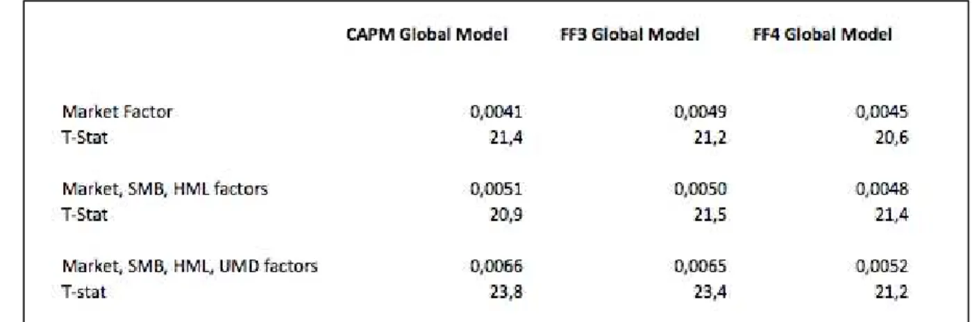
All the Alphas deriving from the time-series regressions are statistically different from zero (see Appendix Table I).
We obtain the lowest pricing errors when we use only the Market local factor as a test asset. In
particular, we found an average Alpha of 0.0041, 0.0049 and 0.0045 for the CAPM, FF3 and FF4 model, respectively.
We have compared the average absolute Alphas derived from the three models during all the period of our analysis, and we can clearly see that CAPM outperformed the other models from 1999 on (Figure I).
Figure I
If we use as test asset the Market local factor and the SMB and HML factor, the FF3 model 0.000
0.002 0.004 0.006 0.008 0.010 0.012 0.014
1994 1995 1996 1997 1998 1999 2000 2001 2002 2003 2004 2005 2006 2007 2008 2009 2010 2011
ABSOLUTE AVERAGE ALPHA ON CAPM, FF3 AND FF4 MODEL
However, looking at all global models and all different test assets we cannot conclude that there is a clear downward trend of Alpha, since the existence of a trend is considerably influenced by
the period we are specifically considering. The same conclusion holds when we consider other test assets (see Appendix fig. II –III).
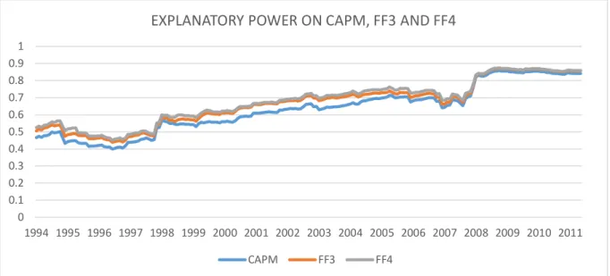
After the Pricing Error, we proceed to the Explanatory Power analysis.
Table II reports the time-series R2 of the CAPM, FF3 and FF4 model for the three different test
assets (see Appendix). When we consider as test asset only the Market factor, we obtain the highest R2: 63%, 67% and 68% for the CAPM, FF3 and FF4 model, respectively.
Moreover, the results clearly suggest that there is a rise over time in the R2. In fact, dividing
the sample in two parts, the R2of the sample from 1994 to 2003 is lower than the one from 2003
to 2012. This result holds considering all the different test assets and all the global models (see Appendix Table III). For example, using the Market as a test asset, the R2 is 52%, 56% and
58% in the first sub-sample and 74%, 77% and 78% in the second sub-sample, for the CAPM, FF3 and FF4 model, respectively.
Figure II
The R2 shows a stable upward trend from 1997 to 2011, with the exception of the years 2006
and 2007. Similar trends are showed when we use other different test assets (see Appendix Fig. IV-V).
In economic terms, this suggests that the power of the global asset pricing models to explain the local factors has improved over our sample period.
5.2 Cross-sectional Results
We performed the cross-sectional analysis for three different test assets and for every test asset
we used as a right-hand variable the CAPM, the three factor model and the four factor model. Comparing all the results, we found that when we use as a test asset the Market local factor, the
SMB factor and the HML factor, we were able to obtain the statistical significance for more coefficients compared to the results obtained using the other test assets. Therefore, we decided to focus on this specific test asset (see Appendix Tab. IV). In particular, we want to check if
the ability of the global models to explain the local factors is improving over time by analysing 0 0.1 0.2 0.3 0.4 0.5 0.6 0.7 0.8 0.9 1
1994 1995 1996 1997 1998 1999 2000 2001 2002 2003 2004 2005 2006 2007 2008 2009 2010 2011
EXPLANATORY POWER ON CAPM, FF3 AND FF4
observations (the number of the countries), the monthly R2 in the cross-sectional regressions
varies considerably, therefore we are not able to draw any conclusion.
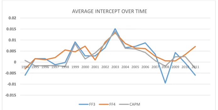
All the intercepts are statistically significant and equal to 0.0027, 0.003 and 0.005 for the
CAPM, FF3 and FF4 model, respectively. The T-statistics of the intercepts are 3.6, 3.4 and 5.7 for the CAPM, FF3 and FF4 model, respectively. Considering all the period, CAPM outperformed the FF3 and the FF4 model in terms of intercept.
Since these results are obtained by doing an average of all the intercepts of every model through all our sample period, we have then examined the changing over time of the intercepts (Fig.
VI).
We can identify an average uptrend from 1994 to 2003 followed by a downtrend until 2007 in
all the models. In the last years of our sample the intercept varies considerably in all the models. However, as for the time-series Alpha analysis, we cannot conclude that the error price decreases and that the models improve over time.
Figure VI
-0.015 -0.01 -0.005 0 0.005 0.01 0.015 0.02
1994 1995 1996 1997 1998 1999 2000 2001 2002 2003 2004 2005 2006 2007 2008 2009 2010 2011
AVERAGE INTERCEPT OVER TIME
The slope of the Market factor is not significant on the CAPM model (T-Stat 1.4) and it is
significant only at a 10% confidence level on the three factor model (T-Stat 1.8). The slope is instead significant in the four factor model (T-Stat 2.4) and it is positive related to the local factors (0.006).
Even if on the three factor model the market coefficient is statistically significant only at a 10% confidence level, we still have decided to compare how it changes over time of it with the one
of the four factor model to see if the models improved over time.
In order to validate the models, the coefficient of the market factor should be equal to the
average Market global factor. The average Market global factor is 0.0085 which is higher than the two coefficients of the models (0.004 and 0.006), which means that the market underperformed. However, when we study the performances dividing the period in two
sub-samples, we can see a catch-up between the slopes and the average Market global factor. The average slopes considering the period May 2003 – February 2012 are equal to 0.0067 and
0.0061 for the three factor model and the four factor model, respectively. The T-statistic of the coefficients are 2.3 and 1.7, respectively.
The SMB factor is not significant in both the three factor and four factor models considering the entire period of our dataset. Considering only the most recent sub-sample, the SMB factor
is significant in the four factor model at a 10% level (t-stat = 1.8) and has a negative sign (-0.0026). The average global SMB factor is equal to -0.003 which is very similar to the result
firm effect”, the tendency of small firms to present an abnormal excess returns with respect to
the big ones.
Regarding the HML slope the results are quite different between the two models and even if we consider the two-subsamples separately they do not present a significant catch up with the
HML global factor. The slope equals to 0.011 (T-stat 2.5) and -0.004 (T-stat -3.3) in the three factor model and four factor model, respectively. The average global HML factor equals to
0.0041.
In conclusion, we observe that the capacity to price the slopes of the factors depends on the test
asset, on the global model, and on the sample period used and that the coefficients do not match with the average global factors.
6.
Conclusion
Recent studies proved that empirical local factor models outperform global factor models in predicting stock returns. In our research we want to see whether and how much global factor models explain local factor and whether this ability is increasing over time. In order to do so,
we use both a time series and a cross sectional analysis regressing the local factors on the betas of the previous month derived from the time-series analysis. We construct three global models
to price local factors: the CAPM, the three factor model and the four factor model.
From the time series analysis, we reach two key results. First, the pricing error is statistically significant in all the models and does not show an improvement over time. Second, in terms of explanatory power, our results suggest a strong increase over time that holds for all the models
power to explain local factors over time. Similar results are reached by Petzev et al.’s research (2016).
From the cross sectional analysis, we reach the same conclusion as for the time-series in terms of pricing error, in fact we cannot conclude that there is a decrease of Alpha over time.
Moreover, using as test asset the Market, the SMB and the HML factors, we are able to price some global factors. In particular, considering only the data from 2003 to 2011 the coefficients
are more significant in terms of T statistic respect with all the sample data. However, using other test assets we are not able to obtain statistically significant slopes.
In conclusion, despite the perception that nowadays financial markets are highly integrated, the empirical results suggest to be cautious. Local factors should be used for the calculation of the
cost of capital and for other performance attribution calculations.
Moreover, we cannot conclude that there is a catch-up between local factor and global factor
7.
Bibliography
Agénor, P. 2003. “Benefits and Costs of Financial Integration: Theory and Facts”. World Economy, Vol. 26, pp. 1089-1118.
Brusa F., T. Ramadorai, A.Verdelhan. 2015. “The International CAPM Redux”. Working paper, University of Oxford.
Baele, L., A. Ferrando, P. Hördahl, E. Krylova and C. Monnet. 2004. “Measuring Financial Integration in the Euro Area”. ECB Occasional Paper No.14.
Carhart, M. 1997. “On persistence of mutual fund performance”. Journal of Finance 55, pp. 57–82.
Chou, P., R.K Chou, J. Wang. 2004. “On the Cross-section of Expected Stock Returns: Fama-French Ten Years Later”. Finance Letters, 2 (1), pp. 18-22.
Fama, E. F., K. R. French. 1992. “The Cross-Section of Expected Stock Returns”. TheJournal of Finance, pp. 427-465.
Fama, E. F., K.R. French. 1993. “Common risk factors in the returns on stocks and bonds”.
Journal of Financial Economics 33, pp. 3–56.
Fama, E. F., K. R. French. 1996. “Multifactor Explanations of Asset Pricing Anomalies”. The Journal of Finance, pp. 55-84.
Fama, E. F., K. R. French. 2012. “Size, Value and Momentum in International Stock Returns”.
Journal of Financial Economics, 105, pp. 457-472.
Koedijk, K. G., K. Clemens, P. Schotman, M.Van Dijk. 1999. “The Cost of Capital in International Financial Markets: Local or Global?”. Journal of International Money and Finance, 905-929.
Petzev, I., A. Schrimpf, A. F. Wagner. 2016. “Has the Pricing of Stocks Become More Global?”. Swiss Finance Institute Research Paper, pp. 15-48.
Schmidt, P., U. Arx, A. Schrimpf, A.F. Wagner, A. Ziegler. 2015. “Size and momentum profitability in international stock markets”. Swiss Finance Institute Research Paper pp.15-29.
Schwert, G.W. 2002. “Anomalies and Market Efficiency”. Simon School of Business Working Paper No. FR 02-13.
Sercu, P. 1980. “A Generalization of the International Asset Pricing Model”. Revue de
l’Association Française de Finance 1, pp. 91-135.
8.
Appendix
Table I - Average Absolute Alpha in Time Series Analysis
Table II – Explanatory Power in Time Series Analysis
Table IV- Cross Sectional Regressions Estimates using as test asset Market, SMB and HML factors.
Figure II- Time-Series Absolute average alpha on CAPM, FF3, FF4 using as test asset the Market, SMB and HML factors.
0 0.002 0.004 0.006 0.008 0.01
1994 1995 1996 1997 1998 1999 2000 2001 2002 2003 2004 2005 2006 2007 2008 2009 2010 2011
Figure III – Time-Series Absolute average alpha on CAPM, FF3, FF4 using as test asset the Market, SMB, HML and UMD factors.
Figure IV – Time-Series Explanatory Power on CAPM, FF3 and FF4 using as test assets the Market, SMB, HML factors.
0 0.002 0.004 0.006 0.008 0.01 0.012 0.014
1994 1995 1996 1997 1998 1999 2000 2001 2002 2003 2004 2005 2006 2007 2008 2009 2010 2011
CAPM FF3 FF4
0 0.1 0.2 0.3 0.4 0.5 0.6
1994 1995 1996 1997 1998 1999 2000 2001 2002 2003 2004 2005 2006 2007 2008 2009 2010 2011
Figure V –Time-Series Explanatory Power on CAPM, FF3 and FF4 using as test assets the Market, SMB, HML and UMD factors.
0 0.1 0.2 0.3 0.4 0.5 0.6 0.7
1994 1995 1996 1997 1998 1999 2000 2001 2002 2003 2004 2005 2006 2007 2008 2009 2010 2011