A 2-D process-based model for suspended sediment dynamics: a first step towards ecological modeling

(1)

HESSD

12, 1507–1553, 2015

A 2-D process-based model for suspended sediment dynamics:

a first step towards ecological modeling

F. M. Achete et al.

Title Page

Abstract Introduction

Conclusions References

Tables Figures

◭ ◮

Back Close

Full Screen / Esc

Printer-friendly Version

Interactive Discussion

Discussion

P

a

per

|

Discussion

P

a

per

|

Discussion

P

a

per

|

Discussion

P

a

per

|

Hydrol. Earth Syst. Sci. Discuss., 12, 1507–1553, 2015 www.hydrol-earth-syst-sci-discuss.net/12/1507/2015/ doi:10.5194/hessd-12-1507-2015

This discussion paper is/has been under review for the journal Hydrology and Earth System Sciences (HESS). Please refer to the corresponding final paper in HESS if available.

A 2-D process-based model for

suspended sediment dynamics: a first

step towards ecological modeling

F. M. Achete1, M. van der Wegen1, D. Roelvink1,2,3, and B. Jaffe4 1

UNESCO-IHE, Delft, the Netherlands 2

Deltares, Delft, the Netherlands 3

Delft University of Technology, Delft, the Netherlands 4

US Geological Survey Pacific Science Center, Santa Cruz, California, USA

Received: 20 December 2014 – Accepted: 15 January 2015 – Published: 2 February 2015

Correspondence to: F. M. Achete (f.achete@unesco-ihe.org)

(2)

HESSD

12, 1507–1553, 2015

F. M. Achete et al.

Title Page

Tables Figures

◭ ◮

Back Close

Full Screen / Esc

Discussion

P

a

per

|

Discussion

P

a

per

|

Discussion

P

a

per

|

Discussion

P

a

per

|

Abstract

In estuaries most of the sediment load is carried in suspension. Sediment dynamics differ depending on sediment supply and hydrodynamic forcing conditions that vary over space and over time. Suspended sediment concentration (SSC) is one of the most important contributors to turbidity, which influences habitat conditions and ecological

5

functions of the system. A robust sediment model is the first step towards a chain of model including contaminants and phytoplankton dynamics and habitat modeling.

This works aims to determine turbidity levels in the complex-geometry Delta of San Francisco Estuary using a process-based approach (D-Flow Flexible Mesh software). Our approach includes a detailed calibration against measured SSC levels, a sensitivity

10

analysis on model parameters, the determination of a yearly sediment budget as well as an assessment of model results in terms of turbidity levels for a single year (Water Year 2011). Model results shows that our process-based approach is a valuable tool in assessing sediment dynamics and their related ecological parameters over a range of spatial and temporal scales. The current model may act as the base model for a chain

15

of ecological models and climate scenario forecasting.

1 Introduction

Rivers transport water and sediments to estuaries and oceans. Sediment dynamics will differ depending on sediment supply and hydrodynamic forcing conditions varying over space and over time. Many river basins are subject to slow morphodynamic

adap-20

tation due to (gradually) changing forcing conditions, ranging from sea level rise and climate change to anthropogenic developments such as reservoir construction in the watershed.

The human impact on sediment production dates from 3000 years ago, and has been accelerating over the past 1000 years due to considerable engineering works (Syvitski

25

(3)

HESSD

12, 1507–1553, 2015

F. M. Achete et al.

Title Page

Tables Figures

◭ ◮

Back Close

Full Screen / Esc

Discussion

P

a

per

|

Discussion

P

a

per

|

Discussion

P

a

per

|

Discussion

P

a

per

|

delivered to the coastal zone varies between 9.3 and 58 Gt yr−1. Estimating the world sediment budget is still a challenge either due to lack of data or detailed model studies in this field (Vörösmarty et al., 2003). Adding to that, there is considerable uncertainty in hydraulic forcing conditions and sediment supply dynamics due to variable adapta-tion timescales over seasons and years (such as varying precipitaadapta-tion and river flow),

5

decades (such as engineering works) and centuries to millennia (sea level rise and climate change).

Examples of anthropogenic changes in sediment dynamics in river basins and estu-aries are manifold, e.g. San Francisco Bay-Delta (Schoellhamer, 2011), Yangtze Estu-aries (Yahg, 1998) and Mekong Delta (Manh et al., 2014). These three systems present

10

similar conditions of anthropogenic forced sediment supply. After an increase in sedi-ment supply (due to hydraulic mining and deforestation respectively) each had a steep drop in sediment discharge (30 %) due to reservoir building and further estuarine clear-ance after depletion of available sediment in the bed. This implies (a) continuous change in sediment dynamics and hence sediment budget in the estuary, (b) change

15

in sediment availability leading to change in turbidity levels.

Turbidity is a measurement of light attenuation in water and it is a key ecological parameter. Fine sediment is the main contributor to turbidity. Therefore suspended sediment concentration (SSC) can be translated into turbidity applying empirical for-mulations. Besides SSC, algae, plankton, microbes and other substances may also

20

contribute to turbidity levels (ASTM International, 2002). High turbidity levels limit pho-tosynthesis activity by phytoplankton and microalgae, therefore decreasing associated primary production (Cole et al., 1986). Turbidity levels also define habitat conditions for endemic species (Davidson-Arnott et al., 2002). We can cite the Delta Smelt as an example seeking for regions where the turbidity is between 12–18 NTU to hide from

25

predators (Bakersville-Bridges, 2004; Brown et al., 2013).

(4)

HESSD

12, 1507–1553, 2015

F. M. Achete et al.

Title Page

Tables Figures

◭ ◮

Back Close

Full Screen / Esc

Discussion

P

a

per

|

Discussion

P

a

per

|

Discussion

P

a

per

|

Discussion

P

a

per

|

To assess the aforementioned issues, the goal of this work is to provide a detailed analysis of sediment dynamics concerning (a) SSC levels, in the Sacramento–San Joaquin Delta (Delta) area, (b) sediment budget and (c) translate theses results in turbidity levels, by means of a two dimensions in the horizontal, averaged in the vertical dimension (2-DH), process-based, numerical model. This process-based model will be

5

able to quantify high resolution sediment budgets and SSC, both in time (∼days) and

space (∼10s–100s of m). We selected the Delta area as a case study, since the area

has been well monitored so that detailed model validation can take place, it hosts endemic species, and allow us to use a 2-DH model approach. The SSC model results are compared to in situ measured SSC data. The calibration process assesses the

10

sensitivity of sediment characteristics such as fall velocity (w), critical shear stress (τcr) and erosion coefficient (E). The model outputs are the spatial and temporal distribution of SSC (turbidity), yearly sediment budget for different Delta regions, and the sediment export to the bay.

For the first time, a detailed, process-based model is developed for San Francisco

15

Bay-Delta, to focus on the complex Delta sediment dynamics. From this model it is pos-sible to describe the spatial sediment (turbidity) distribution and deposition patterns that are important indicators to assess habitat conditions. Analyzing seasonal and yearly variations in sediment dynamics and translating these into turbidity levels to be used as indicators for ecological modeling (Janauer, 2000), this work fills gap the between

20

the physical aspects (hydrodynamic and sediment modeling) and ecology modeling. Previous work focused on understanding the San Francisco Bay-Delta system through data analysis (Barnard et al., 2013; Manning and Schoellhamer, 2013; McKee et al., 2006, 2013; Morgan-King and Schoellhamer, 2013; Schoellhamer, 2011, 2002; Wright and Schoellhamer, 2004, 2005), while similar work in other estuaries around the world

25

(5)

HESSD

12, 1507–1553, 2015

F. M. Achete et al.

Title Page

Tables Figures

◭ ◮

Back Close

Full Screen / Esc

Discussion

P

a

per

|

Discussion

P

a

per

|

Discussion

P

a

per

|

Discussion

P

a

per

|

2 Background

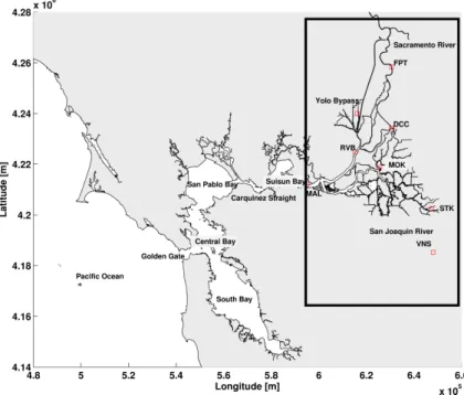
San Francisco Estuary is the largest estuary on the US West Coast. The estuary com-prises San Francisco Bay and the inland Sacramento–San Joaquin Delta (Bay-Delta system), which together cover a total area of 1235 km2 with a mean water depth of 4.6 m (Jassby et al., 1993). The system has a complex geometry consisting of

inter-5

connected sub-embayments, channels, rivers, intertidal flats, and marshes (Fig. 1). The Sacramento–San Joaquin Delta (Delta) is a collection of natural and man-made chan-nel networks and leveed islands, where the Sacramento River and the San-Joaquin River are the main tributaries followed by Mokelumne River (Delta Atlas, 1995). San Francisco Bay has 4 sub-embayments. The most landward is Suisun Bay followed by

10

San Pablo Bay, Central Bay (connecting with the sea through Golden Gate) and, further southward, South Bay.

Tides propagate from Golden Gate into the Bay and most of the Delta up to Sacra-mento (FPT) and Vernalis (VNS) when river discharge is low. Suisun Bay experiences mixed diurnal and semidiurnal tide that ranges from about 0.6 m during the weakest

15

neap tides to 1.8 m during the strongest spring tides. During high river discharge the 2 psu isohaline is located in San Pablo bay while during low river discharge it can go landwards of Chipps Island (westernmost reach of the black rectangle, Fig. 1). The topography highly influences the wind climate in the Bay-Delta system. Wind velocities are strongest during spring and summer presenting afternoon north-westerly gusts of

20

about 9 m s−1(Hayes et al., 1984).

San Francisco estuary collects 40 % of the total Californian fresh water discharge. It has a Mediterranean climate, with 70 % of rainfall concentrated between October and April (winter) decreasing until the driest month September (summer) (Conomos et al., 1985). The orographic lift of the Pacific moist air linked to the winter storms and the

25

(6)

HESSD

12, 1507–1553, 2015

F. M. Achete et al.

Title Page

Tables Figures

◭ ◮

Back Close

Full Screen / Esc

Discussion

P

a

per

|

Discussion

P

a

per

|

Discussion

P

a

per

|

Discussion

P

a

per

|

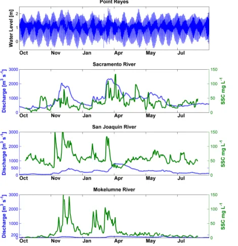
It is important to notice that Sacramento and San Joaquin Rivers, together, account for 90 % of the total fresh water discharge to the estuary (Kimmerer, 2004). The daily inflow to the Delta follows the rain and snowmelt seasonality, with average dry summers with discharges of 50–150 m3s−1 and wet spring/winter reaching peak discharges of 800–2500 m3s−1. The geographic and seasonal flow concentration leads to several

5

water issues related to agricultural use, habitat maintenance and water export. On a yearly average 300 m3s−1of water is pumped from South Delta to southern Califor-nia. The pumping rate is designed to keep the 2 psu (salinity) line landwards of Chipps Island avoiding salinity intrusion in the Delta, allowing the 2-DH modeling approach.

The hydrological cycle in the Bay-Delta determines the sediment input to the system,

10

thus biota behavior. McKee (2006) and Ganju and Schoellhamer (2006) observed that a large volume of sediment passes through the Delta and arrives to the Bay in a yearly pulse. They estimated that in 1 day approximately 10 % of the total sediment volume could be delivered and in extremely wet years up to 40 % of the total sediment volume can be delivered in 7 days. During wet months more than 90 % of the total sediment

15

inflow is supplied to the Delta.

The recent Delta history is dominated by anthropogenic impacts. In the 1850’s hy-draulic mining started after placer mining in rivers became unproductive. Hyhy-draulic mining remobilized a huge amount of sediment upstream of Sacramento. By the end of the nineteenth century the hydraulic mining was outlawed leaving approximately

20

1.1×109m3 of remobilized sediment, which filled mud flats and marshes up to 1 m in

the Delta and Bay (Wright and Schoellhamer, 2004; Jaffe et al., 2007b). At the same time of the mining prohibition, civil works such as dredging and construction of lev-ees and dams started, reducing the sediment supply to the Delta (Delta Atlas, 1995; Whipple et al., 2012).

25

(7)

sed-HESSD

12, 1507–1553, 2015

F. M. Achete et al.

Title Page

Tables Figures

◭ ◮

Back Close

Full Screen / Esc

Discussion

P

a

per

|

Discussion

P

a

per

|

Discussion

P

a

per

|

Discussion

P

a

per

|

iment inflow and outflow, estimated that about two-third of the sediment entering the system deposits in the de Delta (Schoellhamer et al., 2012; Wright and Schoellhamer, 2005). The remaining third is exported to the Bay, and represents on average 50 % of the total Bay sediment supply (McKee et al., 2006), the other half comes from smaller watershed around the Bay (McKee et al., 2013).

5

Several studies have been carried out to determine sediment pathways and to esti-mate sediment budgets in the Delta area (Schoellhamer et al., 2012; Jaffe et al., 2007a; Gilbert, 1917; McKee et al., 2006, 2013; Wright and Schoellhamer, 2005). These stud-ies were based on data analysis and conceptual hindcast models. Although the region has a unique network of surveying stations, there are many channels without

mea-10

suring stations. This might lead to incomplete system understanding and knowledge deficits for the development of water and ecosystem management plans. The monitor-ing stations are located in discrete points hampermonitor-ing spatial analysis. Also, the impact of future scenarios related to climate change (i.e. sea level rise and changing hydro-graphs) or different pumping strategies remains uncertain.

15

2.1 Model description

The numerical model applied in this work is Flow Flexible Mesh (Flow FM). D-Flow FM allows straightforward coupling of its hydrodynamic modules with water qual-ity model, Delft-WAQ (DELWAQ), which gives flexibilqual-ity to couple with the habitat (eco-logical) model. D-Flow FM is a process-based unstructured grid model developed by

20

Deltares (Deltares, 2014). It is a package for hydro- and morphodynamic simulation based on a finite volume approach solving shallow-water equations applying a Gaus-sian solver. The grid can be defined in terms of triangles, (curvilinear) quadrilaterals, pentagons and hexagons, or any combination of these shapes. It is important to note that (orthogonal) quadrilaterals are the most computationally efficient cells. Kernkamp

25

(8)

HESSD

12, 1507–1553, 2015

F. M. Achete et al.

Title Page

Tables Figures

◭ ◮

Back Close

Full Screen / Esc

Discussion

P

a

per

|

Discussion

P

a

per

|

Discussion

P

a

per

|

Discussion

P

a

per

|

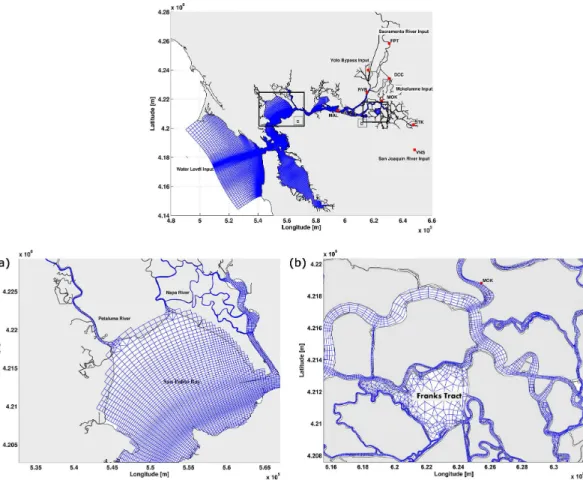
The Bay area and river channels are defined by consecutive curvilinear grids (quadri-lateral). Different resolution grid, the river discharging in the Bay, and channel junctions are connected by triangles (Fig. 2). The average cell size ranges from 1200 m×1200 m,

in the coastal area, to 450 m×600 m in the Bay area down to 25 m×25 m in the Delta

channels. In the Delta, each channel is represented by at least 3 cells in the

across-5

channel direction (Fig. 2). The grid flexibility allows including the entire Bay-Delta in a single grid, but still keeps the computer run times at an acceptable level. It takes 6 real days to run 1 year of hydrodynamics simulation and 12 h to run the sediment module on an 8 cores desktop computer.

We assume that the main flow dynamics in the Delta are 2-D, since no salt-fresh

10

water interactions occur in the Delta and we assume that temperature di_fferences do not govern flow characteristics. D-Flow FM generates hydrodynamic output for off-line coupling with water quality model DELWAQ (Deltares, 2004). Off-line coupling enables faster calibration and sensitivity analysis. DFlow-FM generates time series of the fol-lowing variables: cell link area; boundary definition; water flow through cell link; pointer

15

file gives information concerning neighbors’ cells; cell surface; cell volume; and shear stress file, which is parameterized in DFlow-FM using Manning’sn. Given a network of water levels and flow velocities (varying over time) DELWAQ can solve the advection– diffusion-reaction equation for a wide range of substances including fine sediment, the focus of this study. DELWAQ solves sediment source and sink terms by applying the

20

Krone–Parteniades formulation for cohesive sediment transport (Krone, 1962; Ariathu-rai and Arulanandan, 1978) (Eqs. 1 and 2).

D=ws·c·(1−τb/τd) (1)

E=M·(τb/τe−1) (2)

where D is deposition flux of suspended matter (mg m−2s−1), ws settling velocity of

25

suspended matter (m s−1),cconcentration of suspended matter near the bed (mg m−3),

(9)

HESSD

12, 1507–1553, 2015

F. M. Achete et al.

Title Page

Tables Figures

◭ ◮

Back Close

Full Screen / Esc

Discussion

P

a

per

|

Discussion

P

a

per

|

Discussion

P

a

per

|

Discussion

P

a

per

|

(mg m−2s−1),M first order erosion rate (mg m−2s−1),τecritical shear stress for erosion (Pa).

Note: following Winterwerp (2006) we assume that deposition takes place regardless of the prevailing bed shear stress.τd is thus considered much larger thanτb and the second term in equation (Eq. 1).

5

2.2 Initial and boundary conditions

The Bay-Delta is a well measured system; therefore all the input data to the model are in situ data. Initial bathymetry has 10 m grid resolution, which is based on an ear-lier grid (Foxgrover et al., 2011, http://sfbay.wr.usgs.gov/sediment/delta/), modified to include new data by Wang and Ateljevich (http://baydeltao_ffice.water.ca.gov/modeling/

10

deltamodeling/modelingdata/DEM.cfm) and further refined. The bathymetry is based on different data sources including bathymetric soundings and LiDAR data. The hydro-dynamic model includes real wind, which results from the model described by Ludwig and Sinton (2000). The wind model interpolates hourly data from more than 30 meteo-rological stations into regular 1 km grid cells. Levees and temporal barriers are included

15

in the model considering their deployment time (http://baydeltao_ffice.water.ca.gov/sdb/ tbp/web_pg/tempbsch.cfm).

The hydrodynamic model has been calibrated for the entire Bay-Delta system (see Appendix A and http://www.d3d-baydelta.org/). Initial SSC was set at 0 mg L−1 _over the entire domain. The initial bottom sediment availability defined available mud at

20

places shallower than 5 m b.m.s.l. (below mean sea level) including intertidal mud flats, and sand at places deeper than 5 m b.m.s.l., which are primarily channel regions. This implies that the main Delta channels such as, Sacramento, San Joaquin, Mokelumne are defined as sandy with few mud patches. The smaller channels and the flooded islands such as Franks Tract are initialized with a muddy bottom. DELWAQ does not

25

(10)

HESSD

12, 1507–1553, 2015

F. M. Achete et al.

Title Page

Tables Figures

◭ ◮

Back Close

Full Screen / Esc

Discussion

P

a

per

|

Discussion

P

a

per

|

Discussion

P

a

per

|

Discussion

P

a

per

|

In this study we applied 5 open boundaries. Seaward we set hourly water level time series derived from Point Reyes station (tidesandcurrents.noaa.gov/). The other four landward boundaries are river discharge boundaries at Sacramento River (Freeport), Yolo Bypass (upstream water divergence from Sacramento River), San Joaquin River and Mokelumne River. Studies show that Sacramento River accounts for 85 % of the

5

total sediment inflow to the Delta, while San Joaquin accounts for 13 % (Wright and Schoellhamer, 2005), so it is reasonable to apply 2 sediment discharge boundaries at Sacramento and San Joaquin River. All river boundaries present unidirectional flow, excluding tidal influence.

The river water flow hourly input data at Sacramento River at Freeport (FPT), San

10

Joaquin River near Vernalis (VNS) and Yolo Bypass (YOLO) were obtained from Cal-ifornia Data Exchange Center website (cdec.water.ca.gov/) (Fig. 2). The sediment in-put data, for both inin-put (FPT and VNS) and calibration (SMR, NMR, RVB, MOK, LPS, MDM, STK, MAL) (Fig. 2), was obtained by personal communication from USGS Sacra-mento; this data is part of a monitoring program (http://sfbay.wr.usgs.gov). Since 1998,

15

USGS has continuous measuring stations for sediment concentration which is derived from backscatter sensors (OBS) measurements every 15 min, and nearly monthly cal-ibrated with bottle samples (Wright and Schoellhamer, 2005).

The SSC data that is used to compare to model results are derived from optical backscatter sensors (OBS). This type of sensor converts scattered light from the

par-20

ticles in photocurrent, which is proportional to SSC. To define the rating curve it is necessary to sample water, filter and weight the filter. However, in some locations the cloud of points when correlating photocurrent and filtered weight shows a large scatter. Large scatter leads to errors in translating photocurrent to SSC. These errors are due to (amongst others) particle size, desegregation (cohesiveness, flocculation, organic-rich

25

(11)

HESSD

12, 1507–1553, 2015

F. M. Achete et al.

Title Page

Tables Figures

◭ ◮

Back Close

Full Screen / Esc

Discussion

P

a

per

|

Discussion

P

a

per

|

Discussion

P

a

per

|

Discussion

P

a

per

|

Joaquin Delta these errors can sum up to 39 %, when calculationg sediment fluxes throught Rio Vista.

In this work we modeled the 2011 water year – 1 October 2010 until 30 Septem-ber 2011. First, we ran D-Flow FM for this year to calculate water level, velocities, cell volume and shear stresses. Then, the 1 year hydrodynamic results were imported in

5

DELWAQ which calculated SSC levels.

3 Results

Our focus is to represent realistic SSC levels capturing the peaks, timing and duration, and to develop a sediment budget to assess sediment trapping in the Sacramento– San Joaquin Delta, (Fig. 1, highlighted by the black rectangle). Throughout the

fol-10

lowing sections the results are analyzed in terms of tide averaged results, meaning that the data and model results are filtered to frequencies lower than 2 days. We ap-plied a Butterworth filter with cut offfrequency of 1/30 h−1 as presented in Ganju and Schoellhamer (2006).

3.1 Calibration 15

The results shown below are the derived from an extensive calibration process where the different sediment fractions, w, τcr and E were tested. The first attempt applied multiple fraction settings presented in previous works (van der Wegen et al., 2011; Ganju and Schoellhamer, 2009). However, tests with a single mud fraction proved to be consistent with the data, representative of the sediment budget, and allow a simpler

20

(12)

HESSD

12, 1507–1553, 2015

F. M. Achete et al.

Title Page

Tables Figures

◭ ◮

Back Close

Full Screen / Esc

Discussion

P

a

per

|

Discussion

P

a

per

|

Discussion

P

a

per

|

Discussion

P

a

per

|

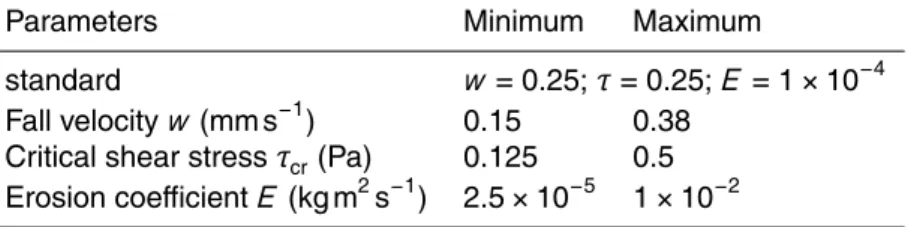
After defining for 1 fraction runs, the sensitivity analysis and metrics helped to choose the standard run presented below, the fraction selected hasw of 0.25 mm s−1,τcr of 0.25 Pa and E of 10−4kg m−2s−1. The same applies to the bed sediment availability defined by 1 mud (shoals) and 1 sand (channels) fraction.

3.2 Suspended sediment dynamics (water year 2011) 5

The 2011 simulation reproduces the SSC seasonal variation in the main Delta regions such as the North (Sacramento River) represented by Rio Vista station (RVB); the South (San Joaquin River) represented by Stockton (STK); central-East Delta repre-sented by Mokelumne station (MOK) and Delta output reprerepre-sented by Mallard Island (MAL) (Fig. 4).

10

All stations clearly reproduce SSC peaks during high river flow periods during November to July and lower concentrations during the remainder of the year (apart from MAL during the July–August period). The good representation of the peak timing indicates that the main Delta discharge event is reproduced by the model as well as the periods of Delta clearance. These two periods are critical for ecological models, and

15

a good representation generates robust input to ecological models. The differences found between the model and data are further discussed in Appendix B.

3.3 Sensitivity analysis

3.3.1 Sediment fraction analysis

We considered one fraction for simplicity and because it reproduces more than 90 %

20

of the sediment budget throughout the Delta as well as the seasonal variability of SSC levels. Although more mud fractions considerably increase running time, several tests with multiple fractions were done to explore possibilities for improving the model results. Including heavier fractions changes the peaks timing and also lowers the SSC curve. Comparing the standard run (w=0.25 mm s−1, τ=0.5 Pa, E =10−4kg m−2s−1 and

(13)

HESSD

12, 1507–1553, 2015

F. M. Achete et al.

Title Page

Tables Figures

◭ ◮

Back Close

Full Screen / Esc

Discussion

P

a

per

|

Discussion

P

a

per

|

Discussion

P

a

per

|

Discussion

P

a

per

|

bottom composition with mud available shallower than 5 m) to another run consider-ing 15 % of heavier fraction (w=1.5 mm s−1) and 30 % of a lighter fraction (fall velocity of 0.15 mm s−1), showed that the peak magnitudes were underestimated but the first peak timing is closer to the data and the spurious peak mid May is lower.

To be able to find the best parameter setting a sensitivity analysis was done varying

5

the main parameters in the Krone–Parteniades formulation (Table 1).

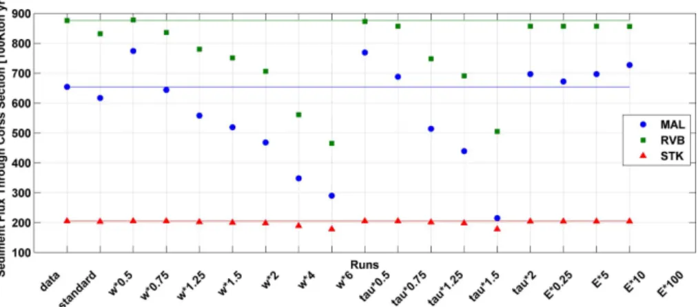
Regarding sediment flux, these tests show that some stations, such as RVB and MAL, are more sensitive to parameter change than others, such as STK (Fig. 5).The model results are most sensitive to the critical shear stress and least sensitive to the erosion coefficient. Analyzing the time series, one concludes that in stations where the

10

fluxes are higher, the change in critical shear stress is less important, since during most of the time the shear stress is already higher than any given critical shear stress.

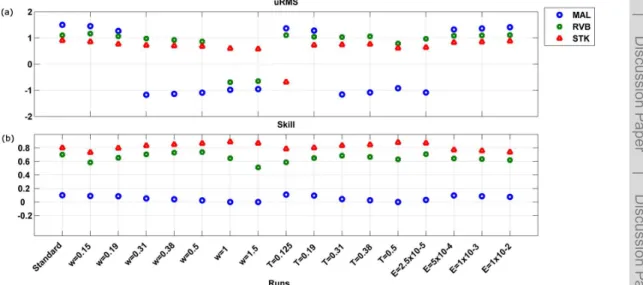
It is important to note that reaching a perfect fit for one station does not mean reach-ing it for the others. We are analyzreach-ing two metrics, the unbiased Root Mean Square Error (uRMSe, Fig. 6) and Skill (Skill, Fig. 6) (Bever and MacWilliams, 2013). The

15

uRMSe analyzes the variability of the model relative to the data, in this case 0 is the case when the model and data have equal variability, positive values indicate more model variability and negative values indicate less model variability.

uRMSe= 1

N N X

i−1

h

XMi−XM XOi−XO

i2 !0.5

(3)

whereNis the time series size,X is the variable to be compared, in this case SSC, and

20

X is the time-averaged value. Subscript “M” and “O” represent modeled and observed values, respectively.

Skill is a single quantitative metric for model performance (Willmott, 1981). When skill equals 1 the model perfectly reproduces the data. The 2 metrics where evaluated at RVB, STK and MAL, representing respectively Sacramento River, San Joaquin River

25

(14)

HESSD

12, 1507–1553, 2015

F. M. Achete et al.

Title Page Abstract Introduction Conclusions References Tables Figures ◭ ◮ ◭ ◮ Back Close

Full Screen / Esc

Printer-friendly Version Interactive Discussion Discussion P a per | Discussion P a per | Discussion P a per | Discussion P a per |

Skill=1− " _N

X

i−1

XMi−XOi

2#, "_XN

i−1

XMi−XO +

XOi−XO 2 # (4)

One notices that changing a parameter can lead to better results in one station but worse in other stations (Fig. 6). The choice of the standard run analyzed throughout the paper comes from this analysis as well as the budget analysis. Following the ar-gumentation from Beven et al. (2011) statistical analyses are needed in order to make

5

a better choice of the model settings. We note that both uRMSe and Skill varies up to 50 % over the different runs.

3.4 Initial bottom composition

To study the importance of initial bottom sediment availability we considered 2 cases; one excluding sediment (concrete bed) and the other by defining available mud at

10

places shallower than 5 m b.m.s.l. including intertidal mud flats and sand at places deeper than 5 m b.m.s.l. being mainly channel regions (standard run). Time series of SSC comparing the 2 cases and data show that bottom composition has virtually no influence on SCC after the first couple of days. This result also applies for different mud fractions availability and opens horizons for modeling less measured estuaries where

15

virtually no bottom sediment data is available.

Another test shows that it is better to initialize the model with a “concrete” bed than with mud available in the entire domain. Initializing the channels with loose mud gen-erates unrealistically high SSC levels through the years, which can take up to 5 years to be reworked.

20

4 Discussion

(15)

HESSD

12, 1507–1553, 2015

F. M. Achete et al.

Title Page

Tables Figures

◭ ◮

Back Close

Full Screen / Esc

Discussion

P

a

per

|

Discussion

P

a

per

|

Discussion

P

a

per

|

Discussion

P

a

per

|

the model results. Although these insights are specific to the San Francisco Bay-Delta system, the same approach can be applied to other estuaries and deltas. The model shows detailed sediment dynamics and the main paths that sediment is transported in the Delta. Sediment flux calculations define the sediment dynamics while gradients in sediment describe the sediment distribution and deposition pattern in the Delta. We

5

also discuss daily and seasonal variation of turbidity levels.

4.1 Spatial sediment distribution

Starting the analysis with the general Delta behavior, during dry periods SSC in the entire Delta is low (<20 mg L−1) and the Delta water is relatively clear. The current model results confirm and compile data showing that the Sacramento River is the main

10

sediment supplier into the Delta (Wright and Schoellhamer, 2004; Schoellhamer et al., 2012). Sacramento River peak flow fills the north and partially fills the central/east Delta with sediment. However, the rest of the Delta keeps quite low levels (∼20 mg L−1) of

SSC all year long. Passing Vernalis (VNS), San Joaquin River main branch flows to the east, however the SSC peak reaches no much further than STK. The west branch goes

15

toward the water pumping stations where to the sediment is pumped out of the system. This behavior reflects in very low SSC in the South Delta (Old River and Franks Tract) region, which are deposition areas.

Three Mile Slough (TMS) and the Delta Cross Channel (DCC) connect the Sacra-mento River with the central and eastern Delta. Model results show that together they

20

carry 60Kton per year of sediment southward. DCC operation defines SSC levels in the eastern/central Delta to a large extent. To show the importance of DCC we run the model twice, one with DCC always open and one always closed. When DCC is open, high SSC Sacramento river water (∼150 mg L−1) flows towards Mokelumne River and

eastern Delta increasing the overall SSC in the area. When it is closed SSC levels in

25

(16)

HESSD

12, 1507–1553, 2015

F. M. Achete et al.

Title Page

Tables Figures

◭ ◮

Back Close

Full Screen / Esc

Discussion

P

a

per

|

Discussion

P

a

per

|

Discussion

P

a

per

|

Discussion

P

a

per

|

from MOK station seawards. In the Sacramento River, the opening decreases SSC levels, by about 10 mg L−1. It affects the river SSC all the way to Mallard Island (Fig. 7). During peak river discharge, Sacramento River sediment reaches Mallard Island in approximately 3 days, Carquinez Straight in 5 days, and the Golden Gate Bridge in approximately 10 days. This timing is proportional to river discharge. However from

5

Mallard Island seawards it is a rough estimate due to the 2-D approximation. The San Joaquin River sediment remains largely trapped in the southern Delta. The flooded islands, breached levees like Franks Tract, present a different behavior. During the entire year the SSC levels are below 15 mg L−1, the river peak discharge signal does not affect them.

10

Sediment flux is a useful tool for a quantitative and qualitative analysis of the sedi-ment path and its derivative gives sedisedi-mentation/erosion patterns. It is defined by the product of water velocity (U), times Cross-sectional area (A) times SSC (C) (Eq. 5).

Fsed=U·A·C (5)

The yearly sediment flux through FPT from model results is 1132 kt yr−1 (thousand

15

metric tons per year) against 1096 kt yr−1 from data, following Sacramento River we have RVB with 832 kt yr−1 _{(994 kt yr}−1_{, data), then MAL with 617 kt yr}−1 _{(654 kt yr}−1₎ (Fig. 8). We calculate that 30 kt yr−1of Sacramento River sediment flows to the eastern Delta through DCC, 30 kt yr−1through TMS and 20 kt yr−1 from Georgina Slough. San Joaquin River carries 490 kt yr−1 _{(498) through VNS, heading to STK with 205 kt yr}−1

20

(190 kt yr−1). It was estimated that 100 kt yr−1was exported through pumping. To close the system in central Delta, the flux through JPT is 126 kt yr−1 (no data) and DCH approximately 0 (no data) (Fig. 8).

4.2 Sediment budget

From the previous section one can see that more sediment enters (∼1600 kt yr−1) than 25

(17)

HESSD

12, 1507–1553, 2015

F. M. Achete et al.

Title Page

Tables Figures

◭ ◮

Back Close

Full Screen / Esc

Discussion

P

a

per

|

Discussion

P

a

per

|

Discussion

P

a

per

|

Discussion

P

a

per

|

inflow and outflow deposits in the Delta. Jaffe et al. (2007b) developed a box model based on bathymetry data to define sediment budget of the Delta and Bay to define sediment availability for ecology purposes. The model results agree with data estima-tions that about two third of the sediment input is retained in the Delta (Schoellhamer et al., 2012; Wright and Schoellhamer, 2005), and it is consistent throughout the years

5

(Cappiella et al., 1999; Jaffe et al., 1998; Wright and Schoellhamer, 2004). Because of the detailed description of the sediment path, it is possible to further understand and describe the sediment budget in Delta sub-regions (north, central and south), com-paring our results to data when available (T. Morgan-King, personal communication, 2012).

10

Besides the overall trend, di_fferent parts of the Delta present di_fferent trap e_fficiency. Model results show that northern Delta (the least efficient) traps∼23 %; central/eastern

Delta traps 32 %, central/western 65 %, and the most efficient is the southern Delta re-gion trapping 67 % of the sediment input. The highest trapping e_fficient regions corre-spond to islands inundated through levee breaching (Wright and Schoellhamer, 2005).

15

From the total Sacramento River sediment input 40 % stays in the northern Delta and about 40 % is exported to Bay area. The remaining 20 % deposits in the central/eastern Delta and only 2 % travel all the way to South Delta. About 70 % of San Joaquin sed-iment deposits in the southern Delta, 10 % go to central Delta, 15 % is exported via Clifton Court pumping facilities and 5 % is exported to the Bay. This transport is

re-20

flected in the bottom composition of the Delta, Sacramento River sediment dominates the northern and central Delta and San Joaquin River sediment dominates the south-ern Delta bottom composition (Fig. 9).

It is possible to divide the sediment budget analysis for the wet and the dry season, since the Delta presents different dynamics for each season. Water year 2011 was

25

(18)

HESSD

12, 1507–1553, 2015

F. M. Achete et al.

Title Page

Tables Figures

◭ ◮

Back Close

Full Screen / Esc

Discussion

P

a

per

|

Discussion

P

a

per

|

Discussion

P

a

per

|

Discussion

P

a

per

|

In this season high SSC gradients are observed in the plume fronts leading to rapid changes in habitat conditions for many species. After the front the high SSC level can last for more than a month, indicating changing in habitat conditions

During the dry season the Delta experiences lower river discharges and SSC levels thus the sediment transport is lower as well. In the dry season SSC levels are more

5

uniform not presenting peaks, at this time the water is clear and the advective flux is lower, which is going to be discussed in the next section.

4.3 Sediment flux analysis

SSC peaks at FPT can be tracked down the estuary. At the RVB station the SSC peak follows the same dynamic as observed at FPT; however, this behavior does not apply

10

for the entire Delta. Schoellhamer and Wright (2005) observed that the river signal is attenuated through the estuary. This attenuation can be understood by analyzing changes in the dominant sediment flux component.

Dyer (1974) decomposed the tidally averaged fluxes in three main components: tidal mean, the advective term; tidal fluctuation, the dispersive term; and the Stokes Drift.

15

This decomposition was possible considering that the measured valued is the sum of a tidally mean component [x], and a fluctuating componentx′_{, so}

x=[x]+x′_, ₍₆₎

substituting in Eq. (5) and simplifying the small contribution terms, three main terms remain (Eq. 7). The first term of Eq. (7) is the advective term, it is the river flow as it

20

is calculated by the mean discharge, area and concentration; the second one is the dispersive term that accounts for tidal pumping, which is the compensation flow for the inward transport of the tidal wave and the Stokes Drift which is the transport due to a variation in the cross-sectional area.

[F]=[U][A][C]+[[U′_C′_][_A_]]₊_[[_U′_A′_[_C_]]] ₍₇₎

(19)

HESSD

12, 1507–1553, 2015

F. M. Achete et al.

Title Page

Tables Figures

◭ ◮

Back Close

Full Screen / Esc

Discussion

P

a

per

|

Discussion

P

a

per

|

Discussion

P

a

per

|

Discussion

P

a

per

|

The model allows for a detailed temporal and spatial analysis of the three flux compo-nents. The temporal analysis are done in 3 steps, the first one considering the whole year and then splitting in the wet and dry season. For the spatial analysis, we defined 4 stations for each river where the first station is dominated by the river flux and the last experience a mix of tidal and river fluxes. The stations were determined following

5

Sacramento River, starting with FPT, followed by RVB down to Mallard Island the delta output and following San Joaquin River from VNS, to STK and MOK. Three Mile Slough (TMS) and San Joaquin Junction (SJJ) represent the Delta smaller channels.

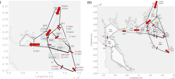
Sacramento River at FPT, the most landward station, experiences no tidal influence so the flux is purely advective. RVB, seaward, experiences tidal fluctuations and the

10

dispersive flux is responsible for 22 % of the total flux; however no Stokes drift flux is present (Fig. 10). On the other hand, Stokes Drift component accounts for 33 % of the total flux in MAL station implying that tides have a bigger influence in this region.

An analogue can be drawn to San Joaquin branch, where VNS and STK experi-ence only advective terms. In MOK and SJJ dispersive (20 and 63 %, respectively) and

15

Stokes flux start (5 and 11 %) to change the total flux (Fig. 10). The analyses of the 3 di_fferent flux components in smaller Delta channels show that river and tidal signals are equally important. In other words the river peak signal is less important inside smaller channels than in rivers. At TMS, the dispersive flow accounts for 60 % of the total flux.

The fluxes analysis shows that there is no change in the Delta net circulation when

20

comparing wet and dry seasons. In other words, there is not a major signal change in the flux signal direction when comparing the seasons. However, there is a change in importance of each flux component.

Figure 10 shows that dispersive flux and Stokes Drift relative contributions vary sea-sonally: when river discharge is high the relative contribution of dispersive flux and

25

(20)

HESSD

12, 1507–1553, 2015

F. M. Achete et al.

Title Page

Tables Figures

◭ ◮

Back Close

Full Screen / Esc

Discussion

P

a

per

|

Discussion

P

a

per

|

Discussion

P

a

per

|

Discussion

P

a

per

|

variation is milder, varying about 10, from 55 % in the wet season and 65 % in the dry. In the dry season the change in fluxes contribution, from advective to dispersive and Stokes Drift, leads to a lower net export of sediment from the Delta, even though the concentrations in the Delta about 30 mg L−1.

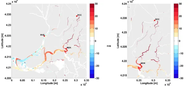
4.4 Sediment deposition pattern 5

The flux change from completely advective to dispersive and Stokes drift sheds some light on the Delta deposition areas. The places where the dispersive flux starts to play a role, near RVB and MOK areas, are the same places where net deposition is ob-served (Fig. 11). Other locations where considerable sedimentation takes place are in flooded islands areas, such as Franks Tract and the Clifton Court. The 2-D model

10

allows determining such areas (Fig. 11).

The San Joaquin River downstream of Stockton experiences high deposition. This finding is confirmed by constant dredging works need to maintain Stockton navigation channel. The river discharge modulates the deposition pattern in the main channels. In the Sacramento River, Rio Vista area (RVB), a rapid deposition takes place just

15

after the peak discharge. Later this deposited sediment is gradually washed away and transported to the mud flats at the channel margins, until the next peak.

At flooded island the sedimentation process is gradually and steady, and is not trans-ported again. The deposition pattern does not change from wet to dry season, except for some small bends in the Sacramento River that goes from eroding (wet) to

deposit-20

ing areas (dry). The deposition pattern provides insight into the best areas for marsh restoration.

4.5 Turbidity

So far the discussion was presented in terms of SSC levels, budgets and fluxes, while ecological analysis is often based on turbidity levels. SSC and turbidity are correlated

25

(21)

HESSD

12, 1507–1553, 2015

F. M. Achete et al.

Title Page

Tables Figures

◭ ◮

Back Close

Full Screen / Esc

Discussion

P

a

per

|

Discussion

P

a

per

|

Discussion

P

a

per

|

Discussion

P

a

per

|

empirically defined for each Delta area. The northern areaa=0.85 andb=0.35; cen-tral/western areaa=0.91 andb=0.29, central/easterna=0.72 andb=0.26; south-erna=1.16 andb=0.27; eastern a=0.914 and b=0.29 (USGS Sacramento, per-sonal communication, 2014).

In this section we present average values for turbidity within a specific Delta region

5

as well as its seasonal and daily variations (Fig. 12). Generally, the mean turbidity lev-els and spatial variations are higher during the wet season than during the dry season. During the wet season, the southern area presents the highest mean value (50 ntu), and deviation (15 ntu), caused by a combination of large sediment supply and low flow velocities. The northern region is the second most turbid area (45±10 ntu), where sed-10

iment transported by Sacramento River flows in the channels, increasing the turbidity levels. The central/eastern region is the least turbid area (5±2 ntu) and, as previously

shown, it presents the highest trapping efficiency of the entire Delta. In the dry season the mean turbidity daily variation decreases in the whole Delta, excepting the cen-tral/eastern region. The opening of the DCC during the dry season lets sediment from

15

the Sacramento River entering these areas, increasing the mean turbidity level. The spatial distribution of the most turbid areas is the same as in the wet season. The daily deviation is mostly proportional to the turbidity level and to the distance from the sea. In the southern and western areas the daily variation is higher during the dry season. It shows that there is a strong tidal signal in these parts of the Delta.

20

5 Conclusions

In this work we make a step towards the understanding and simulating sediment dy-namics from source to sink in a complex estuary. This work shows that it is possible to reproduce the main system sediment dynamics as well as a detailed budget for com-plex areas such as the Delta using a 2-D process based numerical model coupled with

25

(22)

HESSD

12, 1507–1553, 2015

F. M. Achete et al.

Title Page

Tables Figures

◭ ◮

Back Close

Full Screen / Esc

Discussion

P

a

per

|

Discussion

P

a

per

|

Discussion

P

a

per

|

Discussion

P

a

per

|

Overall, the model reproduces the SSC peaks and event timing and duration (wet season) as well as the low concentration in dry season throughout the Delta, except at Mallard where water column is stratified due to salt intrusion. Stratification issues are not solved in a 2-D model; for this reason we are working on a 3-D model in order to include the Bay area, leading to a unique model from source to sink.

5

This work shows that having a few measuring stations at the main input and out-put boundaries allows calculating a detailed sediment budget for the system as well as inferring deposition and/or erosion areas. It is also shown that the model performs better without specifying initial bottom sediment distribution and that simplified sedi-ment inputs result in robust SSC levels, spatial patterns and sedisedi-ment budget. This

10

methodology now can be applied in less measured estuaries.

This model is a step towards an environmental comprehensive model encompassing hydro-, sediment- and ecology dynamics leading to a more robust ecology model. The SSC levels results are ready to be coupled with ecological models, such as light atten-uation model for phytoplankton, mussels and habitat. It also generates input to marsh

15

models in terms of sediment availability. The turbidity and deposition pattern analysis may guide ecologists in future works to define areas of interest and/or venerable areas to be study, as well as guide data collecting efforts.

Our work provides the basis to a chain of models, which goes from the hydrodynam-ics, to suspended sediment, to phytoplankton, to fish, clams and marshes. Using this

20

model it is also possible to explore future scenarios for sea level rise, marsh restoration projects, decrease of sediment input from rivers and changes in water management such as water pumping

Appendix A: Hydrodynamic calibration

The hydrodynamic calibration was carried out for 3 month high river flow conditions

25

(23)

con-HESSD

12, 1507–1553, 2015

F. M. Achete et al.

Title Page

Tables Figures

◭ ◮

Back Close

Full Screen / Esc

Discussion

P

a

per

|

Discussion

P

a

per

|

Discussion

P

a

per

|

Discussion

P

a

per

|

ditions (16 July 2001 until 16 October 2001). All presented data is with respect to NAVD88 (vertical datum), UTM 10 (horizontal datum) and GMT (time reference).

Hourly measured water levels at Point Reyes (tidesandcurrents.noaa.gov/) were used as seaward boundary condition. Landward boundary conditions for the Sacra-mento River were obtained from daily measured river flow data at Freeport (FPT) and

5

for the San Joaquin River near Vernalis (VNS) (cdec.water.ca.gov/). The inflow from the Yolo Bypass was defined as a function of Sacramento River discharge.

Measured data for the Bay area were derived from tidesandcurrents.noaa.gov/, for part of the Delta from the California Data Exchange Centre cdec.water.ca.gov/ and for station with numbers from direct contact with the Department of Water Resources

10

(DWR).

Calibration was carried out by systematically varying the value of the Manning’s co-efficient for different sub-areas of the Bay-Delta system. The calibration data analysis includes (local and time varying) influence of air pressure and wind in the definition of the boundary condition as well as in the calibration data inside the modeling domain.

15

These may account for (part of) the error between measurements and modeling re-sults. Also, the NAVD88 reference is not known for all measurement stations, although tidal water fluctuations may be modeled properly. To circumvent these distortions a bet-ter method to assess the model performance is to focus on wabet-ter level amplitude and phasing of the di_fferent tidal constituents. Boundary conditions, calibration data and

20

model results are thus decomposed by Fourier transformation into tidal components which are then compared. The following table gives the results of this analysis for 34 tidal constituents at Golden Gate (GGT) for high river flow conditions. By far, the main tidal constituents at (GGT) are O1, K1, N2, M2 and S2, with M2 being the largest. The model represents their values quite well. The difference in amplitude is 1.3 % for M2,

25

up to 14 % for O1, but the phasing shows a maximum of only 3 % (O1)).

(24)

HESSD

12, 1507–1553, 2015

F. M. Achete et al.

Title Page

Tables Figures

◭ ◮

Back Close

Full Screen / Esc

Discussion

P

a

per

|

Discussion

P

a

per

|

Discussion

P

a

per

|

Discussion

P

a

per

|

Appendix B: SSC calibration

All stations clearly reproduce SSC peaks during high river flow periods and lower con-centrations during the remainder of the year (apart from MAL during the July–August period). The good representation of the peak timing means that the main Delta event is reproduced by the model as well as the periods of Delta clearance. These two periods

5

are critical for ecological models, and a good representation generates robust input to ecological models. A closer look at Fig. 4 reveals differences between model results and data. Following these differences is discussed station by station in this appendix.

One observes that at RVB, SSC levels are directly proportional to Sacramento River discharge (Fig. B3), and that the model properly represents the water discharge peak

10

intensity and duration. However, in the model, the first peak remobilizes sediment faster than observed in the data. Analyzing the raw data, it is possible to observe a trend of SSC increase which the model overestimates. A probable explanation lies on the initial sediment composition of the bed. Defining the bottom sediment composition does not account for consolidation processes; so the first peak comes after the dry season when

15

the mud in the banks has consolidated. In the simulation case, when river discharge increases, it remobilizes non-consolidated bottom/bank sediment causing an earlier peak than in the data; similar behaviour is observed in STK in December. Sediment trapped in subaquatic vegetation and marshes could be another explanation for the slower increase of the first peak as the model discharges for both stations agree with

20

data (Fig. 4).

Another difference between the data and the model results in RVB is the peak in May (second rectangle, Fig. B1), which is not observed in the data. SSC level at RVB station is directly proportional to water discharge in FPT (Fig. B3, RVB). The May peak is obeserved in FPT and so should have been transported towards RVB just as the

25

(25)

HESSD

12, 1507–1553, 2015

F. M. Achete et al.

Title Page

Tables Figures

◭ ◮

Back Close

Full Screen / Esc

Discussion

P

a

per

|

Discussion

P

a

per

|

Discussion

P

a

per

|

Discussion

P

a

per

|

event and the equipment might be damaged. Other explanations could be a different composition of the suspended sediment properties and/or floculation.

The model underestimates the first and second SSC peaks at MOK. However, the data SSC signal is not consistent with the local water discharge signal. First, we checked that modeled water discharge is reproducing the local conditions, where data

5

is available from mid-February onwards. The last peak in Fig. B1 (mid-March) shows that water discharge, in situ and modeled SSC have the same rage of variation. There-fore the SSC levels are proportional to the local water discharge. Backwards in time, the January SSC data peak is much higher than the water discharge and the SSC level calculated in the model. The same happens in mid-February when no water discharge

10

peak is observed but there is a peak in the SSC data. Again the peaks in SSC could be derived from an error in the measurements or local, diffuse input of sediment such as from local farm waste water or biological activity remobilizing the substrate.

The model represents well the wet season SSC peaks at MAL; however, during the three drier periods of the year the model underestimates SSC levels (Fig. B2). From

15

the scatter plot water discharge vs. SSC (Fig. 13), it is possible to explain the weaker performance of the model during low river flow at MAL. These graphs represent river water discharge in FPT lagged by 2 days to SSC in RVB and MAL. Several time lags were tested, as MAL does not present a reasonable correlation with any of the time lags; it is presented here with the same time lag as the one for RVB. RVB station

20

reflects a positive correlation between river discharge and SSC derived from in situ data and model results. The correlation coefficient (R), statistically shows how two variables are correlated, in RVBR=0.58.

In MAL station R=0.26, showing that there is almost no correlation between river discharge and SSC levels. The low correlation is due to high SSC level in low

wa-25

(26)

HESSD

12, 1507–1553, 2015

F. M. Achete et al.

Title Page

Tables Figures

◭ ◮

Back Close

Full Screen / Esc

Discussion

P

a

per

|

Discussion

P

a

per

|

Discussion

P

a

per

|

Discussion

P

a

per

|

SSC levels at these conditions a 3-D model would be needed to reflect conditions at MAL adequately. With this results we are still able to calculate sediment export, since most of the sediment export occurs in the wet period (McKee et al., 2006), when the model reproduces SSC levels.

Acknowledgements. The research is part of the US Geological Survey CASCaDE climate 5

change project (CASCaDE contribution xx). The authors acknowledge the US Geological Sur-vey Priority Ecosystem Studies and CALFED for making this research financially possible. The data used in this work is freely available on the USGS website (nwis.waterdata.usgs.gov). The model applied in this work will be freely available from http://www.d3d-baydelta.org/.

References 10

Ariathurai, R. and Arulanandan, K.: Erosion rates of cohesive soils, J. Hydr. Eng. Div.-ASCE, 104, 279–283, 1978.

ASTM International: Standards on Disc, Section Eleven, Water and Environmental Technology, PA, USA, 2002.

Barnard, P. L., Schoellhamer, D. H., Jaffe, B. E., and McKee, L. J.: Sediment trans-15

port in the San Francisco Bay coastal system: an overview, Mar. Geol., 345, 3–17, doi:10.1016/j.margeo.2013.04.005, 2013.

Beven, K., Smith, P. J., and Wood, A.: On the colour and spin of epistemic error (and what we might do about it), Hydrol. Earth Syst. Sci., 15, 3123–3133, doi:10.5194/hess-15-3123-2011, 2011.

20

Bever, A. J. and MacWilliams, M. L.: Simulating sediment transport processes in San Pablo Bay using coupled hydrodynamic, wave, and sediment transport models, Mar. Geol., 345, 235–253, doi:10.1016/j.margeo.2013.06.012, 2013.

Brennan, M. L., Schoellhamer, D. H., Burau, J. R., and Monismith, S. G.: Tidal asymmetry and variability of bed shear stress and sediment bed flux at a site in San Francisco Bay, USA, En-25

vironmental Fluid Mechanics Laboratory, Dept. Civil & Environmental Engineering, Stanford University, Stanford, CA, US Geological Survey, Placer Hall, Sacramento, CA, 2002.

(27)

HESSD

12, 1507–1553, 2015

F. M. Achete et al.

Title Page

Tables Figures

◭ ◮

Back Close

Full Screen / Esc

Discussion

P

a

per

|

Discussion

P

a

per

|

Discussion

P

a

per

|

Discussion

P

a

per

|

four climate change scenarios for the Sacramento–San Joaquin Delta, California, Estuar. Coast., 36, 754–774, doi:10.1007/s12237-013-9585-4, 2013.

Cappiella, K., Malzone, C., Smith, R., and Jaffe, B. E.: Sedimentation and Bathymetry Changes in Suisun Bay: 1867–1990, USGS, Menlo Park, 1999.

Cole, B., Cloern, J., and Alpine, A.: Biomass and productivity of three phytoplankton size 5

classes in San Francisco Bay, Estuaries, 9, 117–126, doi:10.2307/1351944, 1986.

Conomos, T. J., Smith, R. E., and Gartner, J. W.: Environmental setting of San Francisco Bay, Hydrobiologia, 129, 1–12, doi:10.1007/BF00048684, 1985.

Davidson-Arnott, R. G. D., van Proosdij, D., Ollerhead, J., and Schostak, L.: Hydrodynamics and sedimentation in salt marshes: examples from a macrotidal marsh, Bay of Fundy, Geo-10

morphology, 48, 209–231, doi:10.1016/S0169-555X(02)00182-4, 2002.

Delta Atlas: Sacramento–San Joaquin Delta Atlas, DWR – Department of Water Resources, California, USA, 1995.

Deltares: D-Flow Flexible Mesh, Technical Reference Manual, Deltares, Delft, 82 pp., 2014. Downing, J.: Twenty-five years with OBS sensors: the good, the bad, and the ugly, Cont. Shelf. 15

Res., 26, 2299–2318, doi:10.1016/j.csr.2006.07.018, 2006.

Dyer, K. R.: The salt balance in stratified estuaries, Estuar. Coast. Mar. Sci., 2, 273–281, doi:10.1016/0302-3524(74)90017-6, 1974.

Ganju, N. K. and Schoellhamer, D. H.: Annual sediment flux estimates in a tidal strait using surrogate measurements, Estuar. Coast. Shelf S., 69, 165–178, 20

doi:10.1016/j.ecss.2006.04.008, 2006.

Ganju, N. K. and Schoellhamer, D. H.: Calibration of an estuarine sediment transport model to sediment fluxes as an intermediate step for simulation of geomorphic evolution, Cont. Shelf. Res., 29, 148–158, doi:10.1016/j.csr.2007.09.005, 2009.

Gibbs, R. J. and Wolanski, E.: The effect of flocs on optical backscattering measure-25

ments of suspended material concentration, Mar. Geol., 107, 289–291, doi:10.1016/0025-3227(92)90078-V, 1992.

Gilbert, G. K.: Hydraulic-Mining Debris in the Sierra Nevada, Professional Paper 105, USGS, Califronia, USA, 154 pp., 1917.

Hayes, T. P., Kinney, J. J., and Wheeler, N. J.: California Surface Wind Climatology, California 30

Air Resources Board, Aerometric Data Division, California, USA, 107 pp., 1984.