Climate bifurcation during the last deglaciation?

www.clim-past.net/8/1127/2012/ doi:10.5194/cp-8-1127-2012

© Author(s) 2012. CC Attribution 3.0 License.

of the Past

Climate bifurcation during the last deglaciation?

T. M. Lenton1, V. N. Livina2, V. Dakos3, and M. Scheffer3

1_{College of Life and Environmental Sciences, University of Exeter, Hatherly Laboratories, Prince of Wales Road,}

Exeter EX4 4PS, UK

2_{School of Environmental Sciences, University of East Anglia, Norwich NR4 7TJ, UK}

3_{Aquatic Ecology and Water Quality Management, Wageningen University, Wageningen, The Netherlands}

Correspondence to:T. M. Lenton (t.m.lenton@exeter.ac.uk)

Received: 5 December 2011 – Published in Clim. Past Discuss.: 12 January 2012 Revised: 4 May 2012 – Accepted: 12 June 2012 – Published: 9 July 2012

Abstract.There were two abrupt warming events during the last deglaciation, at the start of the Bølling-Allerød and at the end of the Younger Dryas, but their underlying dynamics are unclear. Some abrupt climate changes may involve gradual forcing past a bifurcation point, in which a prevailing climate state loses its stability and the climate tips into an alternative state, providing an early warning signal in the form of slow-ing responses to perturbations, which may be accompanied by increasing variability. Alternatively, short-term stochas-tic variability in the climate system can trigger abrupt cli-mate changes, without early warning. Previous work has found signals consistent with slowing down during the last deglaciation as a whole, and during the Younger Dryas, but with conflicting results in the run-up to the Bølling-Allerød. Based on this, we hypothesise that a bifurcation point was approached at the end of the Younger Dryas, in which the cold climate state, with weak Atlantic overturning circula-tion, lost its stability, and the climate tipped irreversibly into a warm interglacial state. To test the bifurcation hypothesis, we analysed two different climate proxies in three Greenland ice cores, from the Last Glacial Maximum to the end of the Younger Dryas. Prior to the Bølling warming, there was a robust increase in climate variability but no consistent slow-ing down signal, suggestslow-ing this abrupt change was proba-bly triggered by a stochastic fluctuation. The transition to the warm Bølling-Allerød state was accompanied by a slowing down in climate dynamics and an increase in climate vari-ability. We suggest that the Bølling warming excited an in-ternal mode of variability in Atlantic meridional overturning circulation strength, causing multi-centennial climate fluctu-ations. However, the return to the Younger Dryas cold state increased climate stability. We find no consistent evidence

for slowing down during the Younger Dryas, or in a longer spliced record of the cold climate state before and after the Bølling-Allerød. Therefore, the end of the Younger Dryas may also have been triggered by a stochastic perturbation.

1 Introduction

Rising variance has also been suggested as an early warn-ing signal prior to abrupt transitions (Carpenter and Brock, 2006), but there is an ongoing debate as to how robust an indicator it is (Dakos et al., 2012; Ditlevsen and Johnsen, 2010). Following the fluctuation-dissipation theorem, it has been argued that both rising variance and rising autocorrela-tion must be detected together to have a robust early warning signal of approaching bifurcation (Ditlevsen and Johnsen, 2010). Furthermore, the ratio of variance to correlation time should remain a constant, set by the noise intensity (assum-ing it is constant) (Ditlevsen and Johnsen, 2010). However, several counterexamples have been provided, where systems show rising autocorrelation prior to bifurcations, but variance does not rise, and indeed may decrease (Livina et al., 2012; Dakos et al., 2012).

Paleo-data approaching past abrupt climate changes can provide a testing ground for these proposed early warning indicators (Livina and Lenton, 2007; Dakos et al., 2008; Ditlevsen and Johnsen, 2010). Alternatively, the indicators can be used to test hypotheses that particular past abrupt cli-mate transitions involved underlying bifurcations. That is the approach we take here.

The last deglaciation was characterised by several abrupt climate changes, notably warming at the start of the Bølling-Allerød period, cooling into the Younger Dryas, and warm-ing at the end of the Younger Dryas (into the Preboreal). The cooling at the onset of the Younger Dryas was less abrupt than the two warming events (Steffensen et al., 2008). The first identification of early warning signals in paleo-climate data was found across the entire deglacial sequence in Green-land ice core (GISP2)δ18O data, and tentatively associated with the Preboreal onset at the end of the Younger Dryas (Livina and Lenton, 2007) (although it could equally have been linked to the Bølling warming). Subsequent work found an early warning signal prior to the Bølling warming in the same GISP2 data, and also discovered early warning prior to the end of the Younger Dryas in marine sediment data from the tropical Atlantic (Cariaco basin) (Dakos et al., 2008).

However, analysis of higher-resolution North Greenland (NGRIP) Ice Core project data failed to find early warning signals prior to any of the abrupt Dansgaard-Oeschger (DO) events during the last ice age, including the Bølling warm-ing (Ditlevsen and Johnsen, 2010). These events have instead been characterised as noise-induced transitions between pre-existing states (or attractors) in the climate system (Ditlevsen and Johnsen, 2010; Livina et al., 2010). Whereas slow forc-ing past a bifurcation point should show the early warnforc-ing signal of critical slowing down, rapid forcing (stochastic or otherwise) between attractors is not expected to (Ditlevsen and Johnsen, 2010; Lenton, 2011).

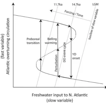
Based on existing results, we suggest a simple conceptual model of the glacial climate in terms of a slow-fast system (Fig. 1). This hinges on a time scale separation between a fast variable – in this case Atlantic meridional overturning circulation (AMOC, coupled to sea-ice and the atmosphere)

Fig. 1.Simple conceptual model of deglacial climate dynamics in terms of a slow-fast system. This incorporates the hypothesis that during the deglaciation there is a gradual approach toward a bifur-cation in which the cold climate state loses its stability.

– and a slow variable – freshwater input to the North At-lantic – in turn linked to the volume of Northern Hemisphere ice sheets. For intermediate values of global ice volume (and, correspondingly, freshwater input to the North Atlantic), the AMOC is assumed to have two alternative states: strong or weak, and the climate is correspondingly warm (inter-stadial) or cold (stadial), particularly in the North Atlantic region. However, the fast variable, AMOC, is assumed to exert some influence on the slow variable, freshwater input to the North Atlantic, such that it slowly destabilises whatever state the climate is in, thus giving the system some propensity to os-cillate (especially in the presence of internal, stochastic vari-ability). Specifically, the strong AMOC, inter-stadial warm state is assumed to melt Northern Hemisphere ice sheets, in-creasing freshwater input to the North Atlantic, whereas the weak AMOC, stadial cold state is assumed to grow North-ern Hemisphere ice sheets, decreasing freshwater input to the North Atlantic. Additionally, it is assumed that even slower factors, namely orbital forcing and associated amplifying changes in global ice volume and atmospheric CO2, which

create the∼100 kyr glacial-interglacial cycles, can alter the stability regime of the AMOC by moving the isocline of the slow variable (Fig. 1) (Crucifix, 2012).

state is assumed to have been stable, consistent with pre-vious work (Livina et al., 2010). The onset of deglaciation then slowly shifted the stability regime until the warm inter-stadial state became marginally stable. The Bølling warm-ing is assumed to have been triggered by a fast perturba-tion around 14.7 ka, and involved an abrupt strengthening of the AMOC. The warmth of the Bølling-Allerød state in turn accelerated Northern Hemisphere ice sheet melt, increasing freshwater input to the North Atlantic and destabilising the strong AMOC. This ultimately contributed to a switch back into cold conditions at the start of the Younger Dryas.

The coldness of the Younger Dryas state then encouraged Northern Hemisphere ice sheets to regrow, slowing global sea-level rise (Bard et al., 2010), and tending to reduce fresh-water input to the North Atlantic. Global deglaciation still proceeded and we suggest it contributed to destabilising the cold climate state (and stabilising the alternative, warm cli-mate state). We hypothesise that an overall reduction in fresh-water input to the North Atlantic during the Younger Dryas caused the AMOC to approach a bifurcation point, in which the weak (stadial) overturning state lost its stability. In sup-port, there is evidence for abrupt strengthening of the AMOC at the end of the Younger Dryas (McManus et al., 2004). Fur-thermore, subsequent meltwater pulses 1B (Bard et al., 2010) and the 8.2 ka event caused only a transient weakening of the AMOC (McManus et al., 2004) and associated cooling, rather than a sustained collapse (as might be expected if the cold climate state was still stable).

The alternative null hypothesis is that the end of the Younger Dryas was a purely noise-induced transition be-tween alternative climate states, with no preceding trend of destabilisation and therefore no early warning. Of course, if a bifurcation was being approached, it would have made it easier for the Younger Dryas to be ended by a stochastic fluc-tuation, so the observed abrupt transition likely did involve internal variability. The key question then is whether it was preceded by any signs of destabilisation.

To test hypotheses for the nature of abrupt climate warm-ing events at the start of the Bøllwarm-ing-Allerød and the end of the Younger Dryas, we extract potential early warning in-dicators from two different climate proxies in three differ-ent Greenland ice-cores: GRIP (Greenland ice core project) (Dansgaard et al., 1993), GISP2 (Greenland ice sheet project 2) (Alley, 2004), and NGRIP (North Greenland ice core project) (NGRIP, 2004). First, we establish whether a sig-nal consistent with slowing down, which has been detected previously across the whole deglaciation (Livina and Lenton, 2007), is present in multiple Greenland ice-core records. Next, we re-examine whether or not there is a signal of slow-ing down prior to the Bøllslow-ing warmslow-ing (Dakos et al., 2008; Ditlevsen and Johnsen, 2010). Then, we examine whether slowing down detected during the Younger Dryas in the trop-ical Atlantic (Dakos et al., 2008) is also present in Green-land. We use two different measures of increasing correla-tion (across different time scales) to look for critical

slow-ing down, and also monitor variance, conductslow-ing a sensitiv-ity analysis for the statistical parameters in our methods, to assess the robustness of the detected signals. In the Discus-sion, we relate our findings to other paleo-data, to process-based models of abrupt deglacial climate changes (Cruci-fix and Berger, 2002; Weaver et al., 2000; Liu et al., 2009; Ganopolski and Rahmstorf, 2001), and to alternative mod-els for the underlying dynamics (Timmermann et al., 2003; Colin de Verdiere, 2006; Crucifix, 2012).

2 Methods

2.1 Data

The GRIP, NGRIP and GISP2 ice cores have recently been synchronised on the Greenland Ice Core Chronology 2005 (GICC05) time scale through the last deglaciation (Ras-mussen et al., 2008), and these data form the basis of our analysis. Critical slowing down, if it occurs, is a property of the slowest decay mode of a system, so we concentrate pri-marily on 20-yr resolution ice core records, which aggregate over shorter time scale variability and fast decay modes.

For each ice core, we examined two proxy records. We focus first on the δ18O water isotope record, which is a proxy for past air-temperature, but can also be influenced by changing water source temperatures and snowfall seasonal-ity. Secondly, we examined the [Ca++

] record, which rep-resents dust from soil-derived carbonates, and thus can cap-ture changes in climate aridity, winds or dust source regions. [Ca++_{] is greatest in cold, dry intervals and fluctuates over} orders of magnitude, falling to very low levels in warm, wet intervals such as the Bølling-Allerød. Hence, it is common to consider loge([Ca++]), which shows a good anti-correlation

withδ18O and exhibits comparable fluctuations. We follow the convention of showing –loge[Ca++] for ease of visual

comparison withδ18O.

We concentrate on the interval from the end of DO event 2∼₂₂.9 ka (22 880 yr b2k on the GICC05 time scale), ap-proaching the Last Glacial Maximum, to the abrupt warming at the end of the Younger Dryas∼₁₁.7 ka (11 740 yr b2k). First, we analyse the whole interval (n= 558 points), includ-ing the abrupt transitions into and out of the Bøllinclud-ing-Allerød. Next, we consider just the run-up to the Bølling warming (DO event 1) ∼14.7 ka (14 740 yr b2k) (n= 408 points). Then, we remove the Bølling-Allerød from the original se-ries, splicing together the run-up to the Bølling warming (stopping 14 760 yr b2k) and the start of the Younger Dryas

∼12.7 ka (12 680 yr b2k) to give a composite series repre-senting just the cold, stadial climate state (n= 455 points). This does not introduce any significant discontinuities into any of the datasets.

resolution loge(Ca) data from GRIP, in order to get a denser

time series. This dataset is on a different time scale and uses different units (but these changes are not critical to the results).

For each dataset, we extracted two different indicators of slowing down: the AR(1) coefficient (ACF-indicator), and a rescaled DFA scaling exponent (DFA-indicator), and also monitored changes in variance.

2.2 Autocorrelation function (ACF-indicator)

Slowing down is measured by an increase in lag-1 autocorre-lation, estimated by fitting an autoregressive model of order 1 (linear AR(1)-process) of the form yt+1t =c·yt+σ ηt, using an ordinary least-squares fitting method, wheret is time,ηt is a Gaussian white noise process of varianceσ2, andcis the autoregressive coefficient;c= exp(−κ1t ), whereκis the de-cay rate of perturbations. The dede-cay rate of the major mode,

κ, tends to zero (i.e. c→1) as bifurcation is approached (Held and Kleinen, 2004). The changing estimated value of the AR(1) coefficient,c, as one moves through a time series is referred to here as the “ACF indicator” – previously termed the “propagator” (Held and Kleinen, 2004).

2.3 Detrended fluctuation analysis (DFA-indicator)

Slowing down causes an increase in short-term memory, which is measured using detrended fluctuation analysis. DFA extracts the fluctuation function of window size,s, which in-creases as a power law if the data series is long-term power-law correlated;F (s)∝sα, where αis the DFA scaling ex-ponent. We consider only the short-term regime, in which as

c→1 and the data approach critical behaviour, the slowing exponential decay is well approximated by a power law in whichα→1.5 (corresponding to a random walk). The DFA exponent is rescaled to give a “DFA indicator” that has been calibrated against the ACF indicator for direct comparison, and reaches value 1 (rescaled from 1.5) at critical behaviour (Livina and Lenton, 2007).

2.4 Variance

We monitor variance, calculated as standard deviation, for comparison with previous work (Ditlevsen and Johnsen, 2010). If the fluctuation-dissipation theorem is applicable, then, as a bifurcation is approached (andκ → 0), variance of the system is expected to increase according to Var(y)

= σ2/2κ, whereσ2 is the variance of the noise (Ditlevsen and Johnsen, 2010). However, variance may not increase if, for example, critical slowing down reduces the capacity of a system to follow high frequency fluctuations, or if a sys-tem becomes less sensitive to stochastic fluctuations as it approaches a threshold (Dakos et al., 2012).

2.5 Detrending

Due to non-stationarities in the paleo-climate records, it is necessary to remove trends before estimating the slowing down indicators or variance. DFA includes an inherent, in-ternal detrending routine (Livina and Lenton, 2007), which is of low-order here and equivalent to simple linear detrend-ing. Before calculating the ACF-indicator or variance, we ex-amined several de-trending approaches (Lenton et al., 2012) and chose Gaussian filtering, which fits a Gaussian kernel smoothing function across the whole record prior to transi-tion (Dakos et al., 2008). Results are similar when Gaussian filtering is applied only within the sliding window (Lenton et al., 2012). The fit is subtracted from the record to obtain the residual data series. Bandwidth for the kernel determines the degree of smoothing, and should be chosen such that it neither over-fits the data nor filters out low frequencies in the record. Here, a default bandwidth of 25 is typically used, but as part of our sensitivity analysis, the bandwidth size of the Gaussian filtering is varied over 5–250 (Dakos et al., 2008).

2.6 Sliding window length

All our indicators are estimated within a sliding window over a time series preceding the onset of a transition. The choice of the sliding window length is a trade-off between time-resolution (data availability) and reliability of the estimate for the indicators. Here, a default value of half the record length is used (Dakos et al., 2008), but sensitivity analy-ses were performed where the length of the sliding window was varied from 25 % of the record length up to 75 % using increments of 20 points. A longer window length leads to more gradual changes in the indicators for the same dataset (Livina et al., 2012).

2.7 Indicator trends

Here, we consider upward trends in both ACF and DFA indi-cators as sufficient to indicate critical slowing down, regard-less of the trend in variance. We use our sensitivity analyses to assess the robustness and strength of the trends in all three indicators. Indicator trends are quantified using the non-parametric Kendall τ rank correlation coefficient (Kendall, 1948). This measures, in the range−_{1 to +1, the strength of}

Fig. 2.Slowing down through the last deglaciation is visible clearly in detrended Greenland ice core δ18O paleo-temperature proxy data:(a)GRIP,(b)GISP2,(c)NGRIP. Example residuals after de-trendingδ18O records 22.88–11.74 ka (n= 558), through the Last Glacial Maximum to the end of the Younger Dryas, using a filter-ing bandwidth of 25, showfilter-ing pronounced slowfilter-ing down, especially after the Bølling warming (∼14.7 ka).

to 1), results should instead be plotted in the middle of the sliding window, and any trend extrapolated forward (with an appropriate error range).

3 Results

Simply detrending theδ18O data from any of the three ice cores over 22.9–11.7 ka and examining the residuals (Fig. 2), one can see clearly that over time, Greenland climate be-comes prone to larger and longer fluctuations. In other words, the climate system becomes more sluggish in response to perturbations as it proceeds through the deglaciation. The slowing down is particularly pronounced during the Bølling-Allerød warm period ∼14.7–12.9 ka, with some signs of a return to faster fluctuations during the Younger Dryas

∼12.9–11.7 ka. In the following sections we examine this signal in more detail.

3.1 The deglaciation as a whole

Analysing the δ18O data over 22.9–11.7 ka, the ACF-indicator (AR(1) coefficient) and standard deviation rise to-gether and roughly in proportion in the GRIP δ18O data (Fig. 3a) and in the GISP2 δ18O data (Fig. 3b), as ex-pected from the fluctuation-dissipation theorem (Ditlevsen and Johnsen, 2010). There is some decoupling between the rises in the ACF-indicator and standard deviation in the NGRIP data (Fig. 3c), in particular, a downward trend in the variance after the Bølling warming, whilst the ACF-indicator continues to rise. In GRIP, NGRIP and GISP2δ18O data, for both the ACF and DFA indicators of slowing down, and the variance, positive trends are robust across a wide range of

window lengths and filtering bandwidths used in the analysis (Fig. 3, colour contour plot insets).

Analysis of the loge[Ca++] data from the three ice cores

over 22.9–11.7 ka also shows positive trends in the ACF and DFA indicators of slowing down, and the variance (Fig. 4). These positive trends are even more robust to varying the window lengths and filtering bandwidths used in the analysis (Fig. 4, colour contour plot insets). Even if one considers raw [Ca++

] data, there remain robust positive trends in ACF and DFA indicators of slowing down, but there are ambiguous trends in variance because [Ca++

] is much less variable in the warm Bølling-Allerød interval, which is toward the end of the time series (results not shown).

Looking across all the results for both proxies (Figs. 3 and 4), increases in the indicators are typically concentrated toward the end of the time series, associated with the Bølling-Allerød in particular. Furthermore, upward jumps in the in-dicators are associated with the Bølling warming, suggest-ing inadequate detrendsuggest-ing of this abrupt transition influences the results. The detrending is improved by picking a shorter filtering bandwidth, e.g. 5 points, and the sensitivity analy-sis (colour contour plots in Figs. 3 and 4) shows that this can eliminate the positive trends in e.g. the ACF-indicator in GRIP and NGIPδ18O, but not in GISP2δ18O or any of the loge[Ca++] datasets. The drawback of such a short filtering

bandwidth is that it also eliminates low-frequency fluctua-tions during the Bølling-Allerød that are clearly visible in the original data and indicative of a slowing down in climate dynamics.

3.2 The run-up to the Bølling warming

This question of whether or not there is any slowing down in climate dynamics prior to the Bølling warming (Dakos et al., 2008; Ditlevsen and Johnsen, 2010) can be roughly an-swered by looking at the example indicators in the run-up to∼14.7 ka in Figs. 3 and 4. This interval 22.9–14.7 ka is analysed in more detail in Figs. 5 and 6.

In the run-up to the Bølling warming in GRIPδ18O data, the ACF indicator shows consistent speeding up, whilst the DFA indicator shows ambiguous trends (Fig. 5a). In GISP2

δ18O data (Fig. 5b), the ACF indicator generally shows slow-ing down, consistent with previously reported results (Dakos et al., 2008) (which are from a shorter interval of GISP2δ18O data on a different time scale), but the DFA indicator shows consistent speeding up. In NGRIPδ18O data (Fig. 5c), the DFA indicator shows consistent speeding up, whilst the ACF indicator gives ambiguous trends, consistent with previous results (Ditlevsen and Johnsen, 2010). All threeδ18O records show robustly rising variance (Fig. 5a–c), whereas previ-ous analyses of NGRIPδ18O suggested no trend in variance (Ditlevsen and Johnsen, 2010).

Analysis of the loge[Ca++] data from the three ice cores

Fig. 3.Indicators of slowing down and changing variance in Greenland ice-coreδ18O paleo-temperature proxy records through the last deglaciation:(a)GRIP(b)GISP2(c)NGRIP. In each case, (Top panel) time series of δ18O data, where analysis spans 22.88–11.74 ka (n= 558), through the Last Glacial Maximum, the Bølling-Allerød, and stopping at the vertical dashed line before the exit from the Younger Dryas. (Left panels) Sensitivity analysis showing values of the Kendall trend statistic for the indicators: (top) ACF, (middle) DFA, (bottom) variance, when varying the sliding window length and (for ACF and variance) the filtering bandwidth used in de-trending. White dots in the contour plots indicate the values of window length and filtering bandwidth used for the example indicators. (Right panels) Example indicators calculated after de-trending, using sliding window length of half the series and (for ACF and variance) a filtering bandwidth of 25: (top) ACF, (middle) DFA, (bottom) variance.

a general increase up to∼17 ka (the time of Heinrich event 1), but often a decline after that. Variance is also generally increasing when considering the data up to∼17 ka but de-clines after that, leading to some ambiguity in the indicators. Looking across all the results for both proxies (Figs. 5 and 6), there is no robust, widespread slowing down prior to the Bølling warming, but there is a robust increase inδ18O vari-ability (Fig. 5), and loge[Ca++] variability also increases up

to∼_{17 ka (Fig. 6).}

3.3 Spliced records of stadial climate dynamics

According to current thinking and following our concep-tual model (Fig. 1), the Bølling-Allerød represents a differ-ent inter-stadial climate state to the cold stadial state that both preceded it and followed it. If this interpretation is cor-rect, then switching between one climate state and another is likely to involve a shift in dynamics that influences the indicators. Hence, to test the hypothesis that the cold, sta-dial climate state approaches a bifurcation on going through the deglaciation, we spliced the Younger Dryas onto what preceded the Bølling-Allerød. Analysis of the resulting com-posite stadial climate datasets shows mixed results (Figs. 7 and 8), which are not radically different to those for the run-up to the Bølling warming (Figs. 5 and 6). In other words, adding on the Younger Dryas does not qualitatively alter the indicator trends and their sensitivity analysis.

Across the threeδ18O datasets (Fig. 7), there is a robust overall rise in variance of the stadial climate state, although at NGRIP (Fig. 7c) there are signs of the variance dropping in the Younger Dryas. In GISP2δ18O data (Fig. 7b), an upward trend in the ACF-indicator is strengthened by including the Younger Dryas, and the example DFA-indicator also starts to rise in the Younger Dryas. Whilst these GISP2δ18O results appear consistent with critical slowing down, they are not reflected in the neighbouring GRIPδ18O or in NGRIPδ18O, where the indicators are generally declining (Fig. 7a, c), with the exception of the DFA-indicator at GRIP.

The loge[Ca++] results are even more varied (Fig. 8). The

ACF-indicators all decline overall with no sign that includ-ing the Younger Dryas starts to reverse the trend. The DFA-indicator rises at GRIP and NGRIP but declines at GISP2. Variance rises strongly at GRIP but less so at GISP2 and declines at NGRIP.

3.4 The Bølling-Allerød and Younger Dryas at annual resolution

When we analyse the Bølling-Allerød and Younger Dryas intervals separately at high resolution, using GRIP loge(Ca)

data (Fig. 9), the results carry the caveat that lag-1 autocor-relation (the ACF-indicator) shows different behaviour in an-nual data, apparently sampling fast decay modes that are not pertinent to bifurcation detection (Lenton et al., 2012). We have more confidence in the DFA-indicator, which shows

comparable behaviour in annual and 20-yr resolution data. It shows no clear trend during the Bølling-Allerød suggest-ing unchangsuggest-ing stability properties (Fig. 9a). This is consis-tent with the onset of the Younger Dryas being caused by a perturbation. During the Younger Dryas there is some weak upward trend in the DFA indicator, but it is sensitive to the window length chosen (Fig. 9b). The strongest signal is a ro-bust decline in variance within both the Bølling-Allerød and the Younger Dryas. In other words, inter-annual climate vari-ability as recorded by loge(Ca) declines during the

Bølling-Allerød and, after rising with the transition into the Younger Dryas, declines again during the Younger Dryas itself. The declining inter-annual variability in the Younger Dryas is at odds with the rising variance at 20-yr resolution (Fig. 8a), which may indicate a shift in power from high to low fre-quencies (spectral reddening) that would be consistent with critical slowing down.

4 Discussion

We hypothesised that there was an approach to bifurcation during the last deglaciation in which the cold stadial climate state lost its stability. Several other dynamical systems mod-els also suggest that the cessation of Dansgaard-Oeschger events on going from the last ice age to the Holocene in-volved an underlying bifurcation in climate dynamics (Tim-mermann et al., 2003; Colin de Verdiere, 2006; Crucifix, 2012). For example, Timmermann et al. (2003) (their Fig. 10) propose a model of a transition from an oscillating AMOC to a convective regime, which is a reversal through a Hopf bifur-cation (from cyclic to fixed point attractor), in which case the signal of critical slowing down would be expected (Thomp-son and Sieber, 2011). Other models suggest a homoclinic bi-furcation or an infinite period bibi-furcation (Colin de Verdiere, 2006). In the case of a homoclinic connection where a cy-cle connects to a saddle, then this should be characterised by the period of the cycle tending to infinity, but this is not particularly helpful, because if the behaviour is cyclic, there is only one instance of the cycle during the deglaciation, so there is no way to say if the cycle is getting longer. Although these various models suggest a climate bifurcation during the last deglaciation, the results we have obtained do not provide convincing support for the bifurcation hypothesis.

Interestingly in the model of Timmermann et al. (2003), entry into a Heinrich event, involving catastrophic iceberg discharge into the North Atlantic, is through a saddle-node (fold) bifurcation, which should show a slowing down signal. In the run-up to Heinrich event H1∼17 ka, the loge[Ca++]

Fig. 5.Indicators of slowing down and changing variance in Greenland ice-coreδ18O paleo-temperature proxy records during the interval after DO event 2 to the Bølling warming (DO event 1):(a)GRIP(b)GISP2(c)NGRIP. Here the analysis spans 22.88–14.74 ka (n= 408), stopping at the vertical dashed line before the Bølling warming. Otherwise panel descriptions are as in Fig. 3.

Fig. 6.Indicators of slowing down and changing variance in Greenland ice-core loge[Ca++] records during the interval after DO event 2 to

Previously reported results showing critical slowing down prior to the Bølling warming in the GISP2 coreδ18O record (Dakos et al., 2008) are not supported by an alternative DFA indicator of critical slowing down. They are neither found in the GISP2 loge[Ca++] record with either ACF or DFA

indi-cators, nor in the neighbouring GRIP coreδ18O record or in the more distant NGRIP coreδ18O record. There is therefore no widespread, robust slowing down tendency prior to the Bølling warming, and no evidence that this abrupt climate change was caused by a bifurcation (in which the cold, dry climate state would have to have lost stability, as hinted at in earlier work (Crucifix and Berger, 2002)). This interpreta-tion is consistent with the return to cold, dry condiinterpreta-tions in the Younger Dryas, which suggests an alternative cold climate state remained stable during the early part of the deglaciation, even though it was not being sampled during the Bølling-Allerød.

The abrupt Bølling warming event appears to have been caused by a stochastic fluctuation (Ditlevsen and Johnsen, 2010). This fluctuation could have taken the form of a rapid, large perturbation. The Atlantic meridional overturning cir-culation (AMOC) had been shut down (McManus et al., 2004) from∼_{17 ka, in response to Heinrich event H1, and}

it resumed abruptly at the Bølling warming (McManus et al., 2004). The triggering fluctuation may have been a sud-den cessation of meltwater discharge into the North Atlantic (Clark et al., 2001; Liu et al., 2009), or meltwater pulse 1A originating from Antarctica (Weaver et al., 2000). However, models require much larger freshwater perturbations to af-fect a transition than data constraints allow (Valdes, 2011), and they generally exhibit much lower internal variability than the real glacial climate. An alternative interpretation, following Ditlevsen and Johnsen (2010), is that the level of glacial climate variability was such that it could (very occa-sionally) tip the system into an alternative warm state. This interpretation is helped by the observation that the strongest signal prior to the Bølling warming is an increase in paleo-temperature variability as recorded byδ18O (Fig. 3). We con-clude that a switch between co-existing cold and warm cli-mate states occurred at the Bølling warming.

The noise-induced switch at the Bølling warming may have been preceded by a bifurcation that re-created a sta-ble, warm climate state, which had lost its stability during the Last Glacial Maximum (Livina et al., 2010). However, the methods applied here would not be able to detect that, as the climate system was only sampling the cold climate state 22.9–14.7 ka, and they focus on deducing changes to its stability properties.

The Bølling warming marked a distinct destabilisation of the climate system. On going through the transition, autocor-relation and variance generally increase in the six ice core records (Figs. 3 and 4). This is not purely a consequence of inadequate detrending of the abrupt transition (although that contributes). There is also a clear shift to lower frequency fluctuations. This suggests the warm climate state that had

been entered was less stable than the preceding cold state of the Last Glacial Maximum. The multi-centennial climate fluctuations during the Bølling-Allerød period can be clearly seen in theδ18O and loge[Ca++] data (Figs. 3 and 4). Their

time scale is consistent with an internal low-frequency mode of variability of the AMOC found in models (Mikolajew-icz and Maier-Reimer, 1990; Park and Latif, 2008). Further-more, decreases in AMOC strength centred on ∼₁₄.1 ka,

∼₁₃.8 ka and ∼₁₃.3 ka have been detected in proxy data (Hughen et al., 2000; Obbink et al., 2010), and linked to tem-perature minima in Greenland (Obbink et al., 2010), North America and Europe (Yu and Eicher, 2001) (known as the intra-Bølling cold period, Older Dryas, and intra-Allerød cold period, respectively). Fluctuations in the eastward rout-ing of freshwater from the Laurentide ice sheet occurred at these times (Clark et al., 2001; Obbink et al., 2010) and may have contributed to AMOC weakening (Obbink et al., 2010), but could equally be viewed as the result of fluctuations in AMOC strength affecting temperatures over the ice sheet (Clark et al., 2001). Thus, we hypothesise that the Bølling warming excited oscillations in the AMOC, coupled to the Laurentide ice sheet.

The overall shift to a less stable, warm climate state may have facilitated further abrupt changes. We find no overall slowing down trend during the Bølling-Allerød period it-self. This is consistent with the onset of the Younger Dryas

∼₁₂.9 ka being caused by a perturbation rather than a bifur-cation. In our characterisation of the climate as a slow-fast system (Fig. 1), the warm Bølling-Allerød climate state in-creased freshwater input to the North Atlantic, thus contribut-ing to its own demise. In reality, this could have been a spo-radic affair, with deglacial meltwater accumulating and then being occasionally purged. This is consistent with the hy-pothesis that the onset of the Younger Dryas∼12.9 ka, was caused by a catastrophic release of deglacial meltwater, prob-ably involving the northward draining of Lake Agassiz into the Arctic Ocean (Murton et al., 2010). Alternative hypothe-ses for the trigger of the Younger Dryas include an extrater-restrial impact (Israde-Alcantara et al., 2012), which might by (slim) chance have hit near enough to have triggered deglacial meltwater release.

Fig. 7.Indicators of slowing down and changing variance of the stadial climate state, joining Greenland ice-coreδ18O paleo-temperature proxy records of the run-up to the Bølling warming to the Younger Dryas:(a)GRIP(b)GISP2(c)NGRIP. Here the data 22.88–14.76 ka are spliced to 12.68–11.74 ka (n= 455) at the point indicated by the vertical dashed line, and the resulting time series is just given an index value (point number). Otherwise panel descriptions are as in Fig. 3.

Fig. 8.Indicators of slowing down and changing variance of the stadial climate state, joining Greenland ice-core loge[Ca++] records of the

Fig. 9.Indicators of slowing down and changing variance in annual resolution GRIP ice core logeCa records of(a)the Bølling-Allerød and (b)the Younger Dryas. Panel descriptions as in Fig. 3.

The Younger Dryas has previously been found to exhibit slowing down in a high-resolution productivity proxy from a sediment core in the tropical Atlantic (Dakos et al., 2008) (Cariaco basin). However, our results from Greenland ice cores do not provide convincing support for the hypothesis that the climate approached a bifurcation at the end of the Younger Dryas. The stadial climate state exhibits no con-sistent slowing down signal in either δ18O or loge[Ca++]

data. Thus, without an obvious proximate trigger perturba-tion, the cause of the abrupt warming at the end of the Younger Dryas ∼₁₁.7 ka remains a puzzle. The transition itself lasted∼60 yr, an order of magnitude slower than the Bølling warming (Steffensen et al., 2008), suggesting some-what different underlying dynamics.

Our failure to find support for the bifurcation hypothesis does not necessarily falsify it. A single realisation of a sys-tem approaching a bifurcation may, by chance, not show the expected indicators of critical slowing down (Kuehn, 2011). Ideally, one should work with an ensemble of realisations of a system to build up better statistics for hypothesis testing. Unfortunately, there is only one realisation of deglaciation for which sufficiently high-resolution climate data are avail-able. However, an alternative study examining whether the triggering of individual Dansgaard-Oeschger events involves any tendency toward bifurcation could make use of the en-semble of over 20 such events in Greenland ice core records.

5 Conclusions

meltwater perturbations did not cause sustained cooling. Fur-ther work should establish a framework of statistical testing against a null hypothesis to try and advance understanding of the dynamics of past abrupt climate changes.

Acknowledgements. Ice core data are from the Centre for Ice and Climate, Niels Bohr Institute, University of Copenhagen, P. D. Ditlevsen provided the high-resolution Ca data and useful ad-vice on comparing it toδ18O. We thank M. Crucifix and T. Kleinen for their constructive critiques which considerably altered the paper. T. M. L. and V. N. L. thank the Isaac Newton Institute for Mathematical Sciences, Cambridge University, for hosting them in the “Mathematical and Statistical Approaches to Climate Modelling and Prediction” programme. T. M. L. and V. N. L. are supported by NERC through the project “Detecting and classifying bifurcations in the climate system” (NE/F005474/1). V. N. L. holds an AXA postdoctoral fellowship. V. D. and M. S. are supported by a Spinoza award from the Dutch Science Foundation (NWO) and a European Research Council (ERC) grant awarded to M. S.

Edited by: U. Mikolajewicz

References

Alley, R. B.: GISP2 Ice Core Temperature and Accumulation Data, NOAA/NGDC Paleoclimatology Program, Boulder, CO, 2004. Alley, R. B., Marotzke, J., Nordhaus, W. D., Overpeck, J. T., Peteet,

D. M., Pielke, R. A., Pierrehumbert, R. T., Rhines, P. B., Stocker, T. F., Talley, L. D., and Wallace, J. M.: Abrupt Climate Change, Science, 299, 2005–2010, 2003.

Bard, E., Hamelin, B., and Delanghe-Sabatier, D.: Deglacial Meltwater Pulse 1B and Younger Dryas Sea Levels Re-visited with Boreholes at Tahiti, Science, 327, 1235–1237, doi:10.1126/science.1180557, 2010.

Carpenter, S. R. and Brock, W. A.: Rising variance: a lead-ing indicator of ecological transition, Ecol. Lett., 9, 311–318, doi:10.1111/j.1461-0248.2005.00877.x, 2006.

Clark, P. U., Marshall, S. J., Clarke, G. K. C., Hostetler, S. W., Lic-ciardi, J. M., and Teller, J. T.: Freshwater Forcing of Abrupt Cli-mate Change During the Last Glaciation, Science, 293, 283–287, doi:10.1126/science.1062517, 2001.

Colin de Verdiere, A.: Bifurcation structure of thermohaline millen-nial oscillations, J. Climate, 19, 5777–5795, 2006.

Crucifix, M.: Oscillators and relaxation phenomena in Pleis-tocene climate theory, Philos. T. R. Soc. A, 370, 1140–1165, doi:10.1098/rsta.2011.0315, 2012.

Crucifix, M. and Berger, A.: Simulation of ocean-ice sheet interac-tions during the last deglaciation, Paleoceanography, 17, 1054, doi:10.1029/2001pa000702, 2002.

Dakos, V., Scheffer, M., van Nes, E. H., Brovkin, V., Petoukhov, V., and Held, H.: Slowing down as an early warning signal for abrupt climate change, Proc. Natl. Acad. Sci. USA, 105, 14308–14312, 2008.

Dakos, V., van Nes, E. H., D’Odorico, P., and Scheffer, M.: Robust-ness of variance and autocorrelation as indicators of critical slow-ing down, Ecology, 93, 264–271, doi:10.1890/11-0889.1, 2012. Dansgaard, W., Johnsen, S. J., Clausen, H. B., Dahl-Jensen, D.,

Gundestrup, N. S., Hammer, C. U., Hvidberg, C. S., Steffensen,

J. P., Sveinbjornsdottir, A. E., Jouzel, J., and Bond, G.: Evidence for general instability of past climate from a 250-kyr ice-core record, Nature, 364, 218–220, 1993.

Ditlevsen, P. D. and Johnsen, S. J.: Tipping points: Early warn-ing and wishful thinkwarn-ing, Geophys. Res. Lett., 37, L19703, doi:10.1029/2010GL044486, 2010.

Elmore, A. C. and Wright, J. D.: North Atlantic Deep Water and cli-mate variability during the Younger Dryas cold period, Geology, 39, 107–110, doi:10.1130/g31376.1, 2011.

Ganopolski, A. and Rahmstorf, S.: Rapid changes of glacial cli-mate simulated in a coupled clicli-mate model, Nature, 409, 153– 158, 2001.

Held, H. and Kleinen, T.: Detection of climate system bifurcations by degenerate fingerprinting, Geophys. Res. Lett., 31, L23207, doi:10.1029/2004GL020972, 2004.

Hughen, K. A., Southon, J. R., Lehman, S. J., and Overpeck, J. T.: Synchronous Radiocarbon and Climate Shifts During the Last Deglaciation, Science, 290, 1951–1954, 2000.

Israde-Alcantara, I., Bischoff, J. L., Dominguez-Vazquez, G., Li, H.-C., DeCarli, P. S., Bunch, T. E., Wittke, J. H., Weaver, J. C., Firestone, R. B., West, A., Kennett, J. P., Mercer, C., Xie, S., Richman, E. K., Kinzie, C. R., and Wolbach, W. S.: Evidence from central Mexico supporting the Younger Dryas extraterres-trial impact hypothesis, Proc. Natl. Acad. Sci., 109, E738–E747, doi:10.1073/pnas.1110614109, 2012.

Kendall, M. G.: Rank Correlation Methods, Charles Griffin & Com-pany Limited, London, 1948.

Kuehn, C.: A mathematical framework for critical transitions: bi-furcations, fast-slow systems and stochastic dynamics, Physica D: Nonlinear Phenomena, 2010, 1–20, 2011.

Lenton, T. M.: Early warning of climate tipping points, Nat. Clim. Change, 1, 201–209, doi:10.1038/nclimate1143, 2011.

Lenton, T. M., Held, H., Kriegler, E., Hall, J., Lucht, W., Rahm-storf, S., and Schellnhuber, H. J.: Tipping Elements in the Earth’s Climate System, Proc. Natl. Acad. Sci. USA, 105, 1786–1793, doi:10.1073/pnas.0705414105, 2008.

Lenton, T. M., Livina, V. N., Dakos, V., van Nes, E. H., and Scheffer, M.: Early warning of climate tipping points from critical slowing down: comparing methods to improve robustness, Philos. T. R. Soc. A, 370, 1185–1204, doi:10.1098/rsta.2011.0304, 2012. Liu, Z., Otto-Bliesner, B. L., He, F., Brady, E. C., Tomas, R., Clark,

P. U., Carlson, A. E., Lynch-Stieglitz, J., Curry, W., Brook, E., Er-ickson, D., Jacob, R., Kutzbach, J., and Cheng, J.: Transient Sim-ulation of Last Deglaciation with a New Mechanism for Bølling-Allerød Warming, Science, 325, 310–314, 2009.

Livina, V. N. and Lenton, T. M.: A modified method for detect-ing incipient bifurcations in a dynamical system, Geophys. Res. Lett., 34, L03712, doi:10.1029/2006GL028672, 2007.

Livina, V. N., Kwasniok, F., and Lenton, T. M.: Potential analysis reveals changing number of climate states during the last 60 kyr, Clim. Past, 6, 77–82, doi:10.5194/cp-6-77-2010, 2010.

Livina, V. N., Ditlevsen, P. D., and Lenton, T. M.: An indepen-dent test of methods of detecting and anticipating bifurcations in time-series data, Physica A: Statistical Mechanics and its Ap-plications, 391, 485–496, 2012.

Mikolajewicz, U. and Maier-Reimer, E.: Internal secular variability in an ocean general circulation model, Clim. Dynam., 4, 145– 156, 1990.

Murton, J. B., Bateman, M. D., Dallimore, S. R., Teller, J. T., and Yang, Z.: Identification of Younger Dryas outburst flood path from Lake Agassiz to the Arctic Ocean, Nature, 464, 740–743, doi:10.1038/nature08954, 2010.

NGRIP: High-resolution record of Northern Hemisphere climate extending into the last interglacial period, Nature, 431, 147–151, 2004.

Obbink, E. A., Carlson, A. E., and Klinkhammer, G. P.: Eastern North American freshwater discharge during the Bolling-Allerod warm periods, Geology, 38, 171–174, doi:10.1130/g30389.1, 2010.

Park, W. and Latif, M.: Multidecadal and multicentennial variability of the meridional overturning circulation, Geophys. Res. Lett., 35, L22703, doi:10.1029/2008gl035779, 2008.

Rasmussen, S. O., Seierstad, I. K., Andersen, K. K., Bigler, M., Dahl-Jensen, D., and Johnsen, S. J.: Synchronization of the NGRIP, GRIP, and GISP2 ice cores across MIS 2 and palaeo-climatic implications, Quaternary Sci. Rev., 27, 18–28, 2008. Scheffer, M., Bacompte, J., Brock, W. A., Brovkin, V., Carpenter, S.

R., Dakos, V., Held, H., van Nes, E. H., Rietkerk, M., and Sug-ihara, G.: Early warning signals for critical transitions, Nature, 461, 53–59, 2009.

Steffensen, J. P., Andersen, K. K., Bigler, M., Clausen, H. B., Dahl-Jensen, D., Fischer, H., Goto-Azuma, K., Hansson, M., Johnsen, S. J., Jouzel, J., Masson-Delmotte, V., Popp, T., Rasmussen, S. O., R¨othlisberger, R., Ruth, U., Stauffer, B., Siggaard-Andersen, M.-L., Sveinbj¨ornsd´ottir, ´A. E., Svensson, A., and White, J. W. C.: High-Resolution Greenland Ice Core Data Show Abrupt Cli-mate Change Happens in Few Years, Science, 321, 680–684, 2008.

Thompson, J. M. T. and Sieber, J.: Predicting climate tipping as a noisy bifurcation: a review, Int. J. Bifurcat. Chaos, 21, 399–423, doi:10.1142/S0218127411028519, 2011.

Timmermann, A., Gildor, H., Schulz, M., and Tziperman, E.: Co-herent Resonant Millennial-Scale Climate Oscillations Triggered by Massive Meltwater Pulses, J. Climate, 16, 2569–2585, 2003. Valdes, P.: Built for stability, Nat. Geosci., 4, 414–416, 2011. Weaver, A. J., Saenko, O. A., Clark, P. U., and Mitrovica, J. X.:

Meltwater Pulse 1A from Antarctica as a Trigger of the Bølling-Allerød Warm Interval, Science, 299, 1709–1713, 2000. Wiesenfeld, K. and McNamara, B.: Small-signal amplification in

bifurcating dynamical systems, Phys. Rev. A, 33, 629–642, 1986. Wissel, C.: A universal law of the characteristic return time near thresholds, Oecologia, 65, 101–107, doi:10.1007/bf00384470, 1984.