Unsteady effects at the interface between impeller-vaned diffuser in a low pressure centrifugal compressor

Unsteady effects at the interface between impeller-vaned

diffuser in a low pressure centrifugal compressor

Sterian DANAILA

, Mihai Leonida NICULESCU*

*Corresponding author

1

Faculty of Aerospace Engineering,

“POLITEHNICA” University of Bucharest,

1 Polizu, sect. 1, 011061, Bucharest, Romania

[email protected]

*

INCAS

‒

National Institute for Aerospace Research “Elie Carafoli”,

B-dul Iuliu Maniu 220, 061126, Bucharest, Romania

[email protected]

Abstract: In this paper, Proper Orthogonal Decomposition (POD) is applied to the analysis of the unsteady rotor-stator interaction in a low-pressure centrifugal compressor. Numerical simulations are carried out through finite volumes method using the Unsteady Reynolds-Averaged Navier-Stokes Equations (URANS) model. Proper Orthogonal Decomposition allows an accurate reconstruction of flow field using only a small number of modes; therefore, this method is one of the best tools for data storage. The POD results and the data obtained by the Adamczyk decomposition are compared. Both decompositions show the behavior of unsteady rotor-stator interaction, but the POD modes allow quantifying better the numerical errors.

Key Words: Unsteady Rotor-Stator Interaction; Adamczyk decomposition; POD; CFD; Compressor, URANS, Flow Field Reconstruction.

1. INTRODUCTION

In the centrifugal compressors, the fluid flow is very complicated due the unsteady and turbulence effects, having time scales that vary considerably. This complexity makes difficult, both experimental and numerical analysis. Usually, in the practical applications, in the reference frame linked to the studied row, a steady flow is assumed. Furthermore, one can decompose the flow in two components: the main flow and the secondary flow,

respectively. The second flow corresponds to the physical flow with non-zero rotor velocity. In the secondary flow, vortices generate the losses due to the entropy increase, leading to three-dimensional behavior of the flow. C. Dano [1] identifies the sources of unsteady phenomena in turbomachinery flows. Because the rotor-stator interaction can affect dramatically the turbomachinery performance, in this paper we’ve paid a special attention to the matter. Most researchers who have studied this interaction from the numerical point of view focused their research on transonic turbomachinery; therefore, there is very few information about the rotor-stator interaction for low velocity turbomachinery. Moreover, a recent study [2] showed important discrepancies between experimental and numerical results for a low-pressure centrifugal stage. Unfortunately, this study did not succeed to identify the effects that caused the major discrepancies between experimental and numerical. Up to now, the Fourier transform is a common tool for the analysis of periodic and non-periodic signals. Some recent studies [3, 4] clearly showed that POD is a more efficient method to extract the dominant modes involved in unsteady flow field. Unfortunately, these studies applied POD

only for one-dimensional decompositions. In order to take the full advantage of POD method, we have applied it for decomposingthe full three-dimensional flow field. For this reason, we have considered that it is useful to study the rotor-stator interactions in a low-pressure centrifugal stage, using both Adamczyk and proper orthogonal decomposition.

2. NOMENCLATURE

e internal energy (J/kg) fe external acceleration (m/s

2

)

Fx, Fy, Fz vectors of convective components of flux Gx, Gy, Gz vectors of diffusive components of flux h static enthalpy (J/kg)

I rothalpy (m2/s2) p static pressure (Pa) r radius (m)

R gas constant (J/(kgK)) S vector of source term T static temperature (K) t time (s)

u, v, w Cartesian components of velocity (m/s) V absolute velocity (m/s)

W relative velocity (m/s) ijk Levi-Civita symbol

 thermal conductivity (W/(mK))  dynamic viscosity (kg/(ms)) t eddy viscosity (kg/(ms))

 azimuthal (circumferential) angle (rad)  static density (kg/m3)

 shear stress tensor (Pa)  angular velocity (rad/s) Subscript

R rotor t turbulent Superscript

eff effective (laminar + turbulent)

3. GOVERNING EQUATIONS

For a three-dimensional rotating Cartesian coordinate system, the unsteady Reynolds-averaged Navier-Stokes equations using the Favre averaging (a mass-weighted averaging) could be written in the conservative form as [5,6]

 

ρ _      i i u x t (1)

 









eff ij j i j i j i p x f u u x u

t ρ ρ ρ  τ  δ

 

 

_









































u

x

T

x

q

u

f

I

u

x

E

t

ρ

ρ

ρ

κ

τ

where energy E and rothalpy I are defined by:

2 2 2 2 ri v i w e

E   (4)

2 2 2 2 ri i v w h

I   (5)

k j ijk ri ri i

i u v v x

w   , 



According to the Boussinesq hypothesis and Stokes postulates and hypothesis for a Newtonian fluid, the shear stresses eff may be written as:









k k t i j j i t eff ij

x

u

x

u

x

u

_

_

_













































3

2

The Sutherland’s formula could be used to determine the dynamic viscosity  as

function of temperature, while the eddy viscosity t is computed with a turbulence model.

For gases, the external force fe due to the gravitational acceleration is very small,

therefore it can be neglected. Moreover, we can assume that the heat conduction is the single heat source. The pressure is obtained from the equation of state,

RT

p



4. NUMERICAL SIMULATION

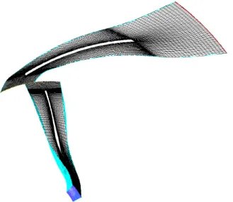
The numerical simulations of the three-dimensional viscous flow were carried out on a centrifugal compressor designed, manufactured and tested by COMOTI, with commercial CFD code FLUENT that is based on finite volume method where each unknown takes an average value on each discretization cell. The computational domain generated in Gambit was split into eight blocks to facilitate the building of a fully structured mesh as shown in Fig. 1. The mesh for which, the results are given, has about 253 000 hexahedral cells for the impeller passage and 127 000 hexahedral cells for the vaned diffuser passage.

turbulent viscosity ratio t/ is 10 and the flow is normal to inlet. At the outlet, a uniform

static pressure (156 000 Pa) is imposed. At the left and right sides of computational domain, the rotational periodic boundary conditions are imposed. All the walls have been assumed adiabatic. The shaft speed of impeller is 14 915 rpm.

Fig. 1 Computational domain of centrifugal compressor

5. ADAMCZYK DECOMPOSITION

Non-uniformities and unsteadiness due to the rotor-stator interaction introduce major complexity in the analysis of the turbomachinery flow field. This problem can be considerably simplified if we apply the method of Adamczyk [9, 4] that proposed the decomposition of an arbitrary field variable u associated to a turbomachinery in four contributions through the successive application of averaging operators:



   

 



















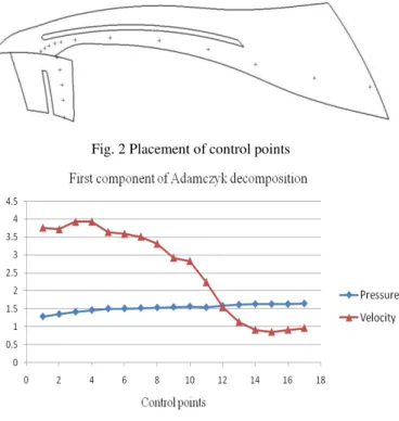
As it follows, we will give some results for some control points placed in a section at mid height of blade of vaned diffuser, at the middle distance between the blade and the right periodic, as shown in Fig. 2. The numbering of these control points is from upstream to downstream.

Fig. 2 Placement of control points

Fig. 3 First component of Adamczyk decomposition for static pressure normalized by inlet static pressure and absolute velocity normalized by inlet absolute velocity

The first component of Adamczyk decomposition for static pressure and absolute velocity, at considered control points is shown in Fig. 3. One sees that the compression process is smooth while the absolute velocity has big variations especially in the first part of vaned diffuser where the strong deceleration triggers a huge jet-wake region accompanied by boundary layer separation on suction side of vaned diffuser blade. These phenomena generate huge nonuniformities in the absolute velocity field as shown in Figs. 4 and 5, which induce important total pressure losses. For this reason, the compression process is very slow in the last part of vaned diffuser.

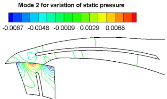
Furthermore, the rectangular trailing edge of vaned diffuser blade generates additional nonuniformities, which are shown in Fig. 5 and losses. The homogenization process of flow begins after the trailing edge of vaned diffuser blade and it is accompanied by significant total pressure losses. For this reason, the air compression is very weak downstream of the trailing edge. The second component of Adamczyk decomposition for static pressure clearly shows the stagnation point, the rarefaction near leading edge, as well as the interaction among the blades of vaned diffuser in the region where the distance among blades is small as shown in Fig. 6.

Fig. 4 Second and third component of Adamczyk decomposition for static pressure normalized by inlet static pressure and absolute velocity normalized by inlet absolute velocity

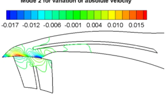
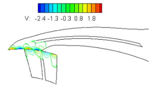
Fig. 5 Isolines of second and third component of Adamczyk decomposition for absolute velocity in the section from the middle height of vaned diffuser

Fig. 6 Isolines of second and third component of Adamczyk decomposition for static pressure in the section from the middle height of vaned diffuser

6. PROPER ORTHOGONAL DECOMPOSITION

In the field of fluid mechanics, two approaches have been used for the POD. Historically the method of Continuous POD (or the classical method) of Lumley [10] proceeded by the Snapshot POD of Sirovich [11]. More information regarding the application of the proper orthogonal decomposition in the analysis of turbulent flows together with a detailed bibliography is given in [12]. In this paper, we used the Snapshot POD because it is much more efficient from the numerical point of view. The POD is a method that reconstructs a data set from its projection onto an optimal base. Besides using an optimal base for reconstructing the data, the POD does not use any prior knowledge of the data set. It is because of this that the basis is only data dependent and this is reason that the POD is used also in analyzing the natural patterns of the flow field. For the reconstruction of the dynamic behavior of a system the POD decomposes the data set in two parts: a time dependent part, ak

(t), that forms the orthonormal amplitude coefficients and a space dependent part, k(x) that

 

 

 

u x t a t  x







where M is the number of time instant observations in the data set. We denote the error of the reconstructed data set as:

   

 

 

x t u x t a t x

 



 



The base from which the data set is reconstructed is said to be optimal in the sense that the average least squares truncation error is minimized for any given number (

m



M





m

    (12)

where the . is the ensemble average and

 

It was shown that the minimization condition for error (x,t) translates into maximum condition for:





This maximization can be proven to take place if the time independent base

functions (

x

) are obtained from the Fredholm integral equation:





 

 

1

, ' ' '

M

ij j i

j

R x x  x dx  x



 



where Rij is the correlation kernel. In this way, we transform this into an eigenvalue problem

and k is the eigenvalue corresponding of the eigenvector k. Because we can consider the

inner product as being the equivalent of an “energy”, the value of k is linked to the energy

contained in mode k and the optimization process involved can be summarized as: the data

set is projected onto a basis that maximizes the energy content. While in the classical approach of Lumley [10], the correlation matrix is constructed as a space correlation matrix and solving the eigenvalue problem, we obtain directly the eigenvectors as the spatial modes and then use them in order to obtain the time-dependent coefficients

 



   



k k

a t  u x t  x (15)

in the Snapshot POD of Sirovich [11], the correlation matrix is a time correlation matrix:

   

1

, , '

V

C u x t u x t dV V





which is of the size of the squareof the snapshots number. From the time correlation matrix, we get the eigenvalues k and time dependent eigenvectors k(t). The spatial eigenmodes that

are time- independent are computed according to the formula:

 

   

,

k k

k t

x t u x t dt

 







k k

   (18)

For the reconstruction of u(x,t), we take into account only a small number of modes that contain the most energy:

 

   

1 ,

m

k k k

k

u x t   t  x 





The processed data are the variations of absolute velocity magnitude and static pressure fields, which represent the fourth term of Adamczyk decomposition according to Eq. 9. These variations were obtained from numerical simulations using the commercial CFD code Fluent. For each period, we took 20 snapshots and the time between adjacent snapshots is of t = 9.5781s; therefore, the Snapshot POD of Sirovich yields 20 eigenmodes for each considered field. The very high efficiency of the proper orthogonal decomposition is clearly underlined in Table 1. The sum of the first two modes represents 90.5% and 95.5% of the total energy, respectively for the variations of static pressure and absolute velocity magnitude fields while the sum of modes 6 to the last mode represents only 0.163% and 0.236% of the total energy, respectively for the variations of static pressure and absolute velocity magnitude fields. Therefore, both variations of static pressure and absolute velocity magnitude fields can be accurately reconstructed using only the first four modes. Furthermore, these results confirm that the base from which the data set is reconstructed is indeed optimal.

Table 1. Fraction of total energy for the most energetic modes

Mode Fraction of total energy for variation of static pressure

Fraction of total energy for variation of absolute velocity

1 6.40E-01 5.49E-01

2 2.65E-01 4.06E-01

3 6.63E-02 2.13E-02

4 1.72E-02 1.58E-02

5 8.97E-03 5.73E-03

6 1.41E-03 7.57E-04

7 6.29E-04 4.50E-04

8 1.60E-04 8.52E-05

9 4.58E-05 7.30E-05

10 4.02E-05 5.25E-05

Fig. 8 Isolines of mode 1 for variation of static pressure in the section from the middle height of

vaned diffuser

Fig. 9 Isolines of mode 2 for variation of static pressure in the section from the middle height of

vaned diffuser

Fig. 10 Isolines of mode 3 for variation of static pressure in the section from the middle height of

vaned diffuser

Fig. 11 Isolines of mode 4 for variation of static pressure in the section from the middle height of

vaned diffuser

Fig. 12 The first four most energetic modes of variation of absolute velocity magnitude field

Fig. 13 Isolines of mode 1 for variation of absolute velocity magnitude in the section from the middle

height of vaned diffuser

Fig. 14 Isolines of mode 2 for variation of absolute velocity magnitude in the section from the middle

height of vaned diffuser

Fig. 15 Isolines of mode 3 for variation of absolute velocity magnitude in the section from the middle

height of vaned diffuser

Fig. 16 Isolines of mode 4 for variation of absolute velocity magnitude in the section from the middle

height of vaned diffuser

contain the information regarding the interaction between wakes and potential effects as well as the influence of potential effects in the impeller region. From the numerical point of view, they represent the numerical errors that occur at the interface between rotating region and stationary region and due to the rotational periodicity condition as shown in Figs. 15 and 16. Furthermore, one sees that the value of the third mode is not close to zero at the outlet boundary of computational domain as shown in Fig. 12 because we imposed a uniform static pressure on this frontier and this is not too correct according to the theory of characteristics [5, 6]. The analysis of time-dependent coefficients ak(t) (also called modal amplitudes or

Fourier coefficients) allows to see if the neighboring spatial modes could interact or the interaction among them is excluded.

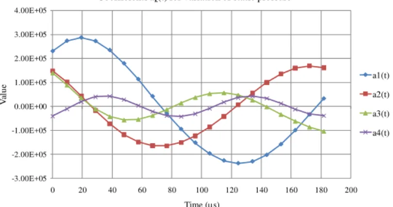
Fig. 17 The time-dependent coefficients ak(t) corresponding to the first four most energetic modes of variation of static pressure field

Fig. 18 The time-dependent coefficients ak(t) corresponding to the first four most energetic modes of variation of absolute velocity field

One expects to be a correlation between spatial modes of variations of static pressure and absolute velocity. However, Figs 17 and 18 suggest that the first mode of variation of static pressure does not correspond to the first mode of variation of absolute velocity; the second mode of variation of static pressure does not correspond to the second mode of variation of absolute velocity and so on. But the periods of the first two time-dependent coefficient ak(t) are very close for both variations of static pressure and absolute velocity.

Furthermore, the periods of a3(t) and a4(t) are also very close for both variations of static

pressure and absolute velocity. These observations suggest that we should couple the first two modes and modes three and four in order to see their physical meaningfulness.

-3.00E+05 -2.00E+05 -1.00E+05 0.00E+00 1.00E+05 2.00E+05 3.00E+05 4.00E+05

0 20 40 60 80 100 120 140 160 180 200

V

al

u

e

Time (s)

Coefficients ak(t) for variation of static pressure

a1(t) a2(t) a3(t) a4(t)

-1.00E+03 -8.00E+02 -6.00E+02 -4.00E+02 -2.00E+02 0.00E+00 2.00E+02 4.00E+02 6.00E+02 8.00E+02 1.00E+03

0 20 40 60 80 100 120 140 160 180 200

V

al

u

e

Time (s)

Coefficients ak(t) for variation of absolute velocity

Fig. 19 The coupling of time-dependent coefficients ak(t) corresponding to the first four most energetic modes of variation of static pressure field

Fig. 20 The coupling of time-dependent coefficients ak(t) corresponding to the first four most energetic modes of variation of absolute velocity field

Analyzing Figs. 19 and 20, one suggest the possibility to exist a correlation between the first two coupled modes of variation of static pressure and the first two coupled modes of variation of absolute velocity. However, the following two coupled modes of variations of static pressure and absolute velocity seem to be uncoupled.

7. RECONSTRUCTION

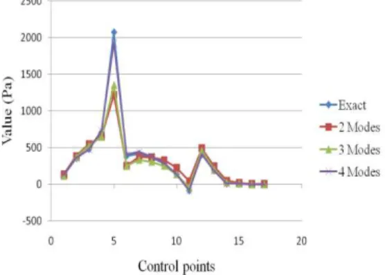
Because the POD is a method that reconstructs a data set from its projection onto an optimal base, we need only four modes to accurately rebuild the variations of static pressure and absolute velocity fields. We will rebuild them for two moments placed at half the period (the number of impeller blades is equal to the number of vaned diffuser blades) as shown in Figs. 21 and 22.

Fig. 21 The first moment for which, the reconstruction is built and isolines of static pressure

computed with commercial code Fluent

Fig. 22 The second moment for which, the reconstruction is built and isolines of static pressure

computed with commercial code Fluent -4.0000E+05

-3.0000E+05 -2.0000E+05 -1.0000E+05 0.0000E+00 1.0000E+05 2.0000E+05 3.0000E+05 4.0000E+05

0 20 40 60 80 100 120 140 160 180 200

V

a

lue

Time (s)

Coupling of coefficients ak(t) for variation of static pressure

a1(t)-a2(t) a3(t)+a4(t)

-1.5000E+03 -1.0000E+03 -5.0000E+02 0.0000E+00 5.0000E+02 1.0000E+03 1.5000E+03

0 20 40 60 80 100 120 140 160 180 200

V

a

lue

Time (s)

Coupling of coefficients ak(t) for variation of absolute velocity

Fig. 23 Reconstruction of variation of absolute velocity magnitude field for first moment

Fig. 24 Reconstruction of variation of static pressure field for first moment

Fig. 25 Reconstruction of variation of absolute velocity magnitude field for second moment

Analyzing the Figs. 23-26, one observes that only four modes are enough toaccurately reconstruct the variations of static pressure and absolute velocity magnitude fields. Furthermore, the points where the field variable u(x,t) has high absolute values are better reconstructed than the points with small absolute values because the data set is projected onto a basis that maximizes the energy content. In other words, points with high energy (information) are reconstructed more accurately than points with low energy.

As it follows, we will reconstruct the variations of static pressure and absolute velocity, in the section from the middle height of vaned diffuser, using all modes, the first two modes and modes three and four, as shown in Figs 27-38.

Fig. 27 Reconstruction of variation of static pressure field for first moment, using all modes (20)

Fig. 28 Reconstruction of variation of static pressure field for second moment, using all modes (20)

Fig. 29 Reconstruction of variation of absolute velocity field for first moment, using all modes (20)

Fig. 30 Reconstruction of variation of absolute velocity field for second moment, using all modes

(20)

Fig. 31 Reconstruction of variation of static pressure field for first moment, using the first two modes

Fig. 33 Reconstruction of variation of absolute velocity field for first moment, using the first two

modes

Fig. 34 Reconstruction of variation of absolute velocity field for second moment, using the first two

modes

Fig. 35 Reconstruction of variation of static pressure field for first moment, using only modes 3 and 4

Fig. 36 Reconstruction of variation of static pressure field for second moment, using only modes 3 and 4

Fig. 37 Reconstruction of variation of absolute velocity field for first moment, using only modes 3

and 4

Fig. 38 Reconstruction of variation of absolute velocity field for second moment, using only modes 3

and 4

The reconstruction clearly shows that the pressure gradient has a secondary role in the absolute velocity field where rotational and Coriolis effects are dominants. According to Bernoulli equation, there is not any correlation between the first two coupled modes of static pressure variation and the first two coupled modes of absolute velocity variation although the coupled time coefficients ak(t) suggested the possibility to exist a relationship between them.

8. CONCLUSIONS

Both Adamczyk and proper orthogonal decompositions have been successfully applied to the decomposition of fully three-dimensional static pressure and absolute velocity magnitude fields obtained from numerical simulations, using the commercial CFD code Fluent.

Both variations of static pressure and absolute velocity magnitude fields can be accurately reconstructed using only the first four modes; therefore, the proper orthogonal decomposition method is a very efficient method for the data storage of unsteady flows. Moreover, thePOD technique is able to capture the relevant features of the unsteady rotor-stator interaction, especially, the potential effects and the interaction between wakes due to the circumferential Coriolis force and blunt trailing edge of impeller blade and potential effects.

The reconstruction clearly shows that the pressure gradient has a secondary role in the absolute velocity field because the rotational and Coriolis effects are dominants. This

conclusion is in concordance with Rochuon’s observations [4].

Furthermore, the POD method clearly shows the numerical errors such as those errors that occur at the interface between rotating region and stationary region because the information exchange does not use the characteristic variables, the reflection of numerical waves at rotational periodic and outlet boundaries as well as their magnitude. In order to obtain more accurate results, we should impose the phase-lagged condition [4,13], which is not yet available in Fluent, on the left and right sides of computational sides, instead of the rotational periodicity condition or to simulate the whole stage [7].

ACKNOWLEDGEMENTS

This paper was presented at the International Conference of Aerospace Sciences "AEROSPATIAL 2012", Bucharest, 11-12 October, 2012 within the section of Aerodynamics.

REFERENCES

[1] C. Dano, Évaluation de modèles de turbulence pour la simulation d’écoulements tridimensionnels

instationnaires en turbomachines, Thèse de doctorat, École Centrale de Lyon, 2003.

[2] P. E. Smirnov, T. Hansen, F. R. Menter, Numerical simulation of turbulent flows in centrifugal compressor stages with different radial gaps, GT2007-27376, Proceedings of ASME Turbo Expo 2007: Power for Land, Sea and Air, Montreal, Canada, 2007.

[3] N. Rochuon, I. Trébinjac, G. Billonnet, An extraction of the dominant rotor-stator interaction modes by the use of proper orthogonal decomposition (POD), Journal of Thermal Science 15 (2) 109-114, 2006. [4] N. Rochuon, Analyse de l’ écoulement tridimensionnel et instationnaire dans un compresseur centrifuge à fort

taux de pression, Thèse de doctorat, École Centrale de Lyon, 2007.

[5] C. Hirsch, Numerical computation of internal and external flow, Volume 2: Computational methods for inviscid and viscous flows, John Wiley and Sons, New York, 1990.

[6] S. Dănăilă, C. Berbente, Numerical methods in fluid dynamics (only in Romanian), Publishing House of Romanian Academy, 2003.

[7] N. Gourdain, S. Burguburu, F. Leboeuf, G. J. Michon, Simulation of rotating stall in a whole stage of an axial compressor, Computers & Fluids 39 (9) 1644-1655, 2010.

[8] P. R. Spalart, S. R. Allmaras, A one-equation turbulence model for aerodynamic flows, AIAA Paper 92-0439, 1992.

[9] J. J. Adamczyk, Model equation for simulating flows in multistage turbomachinery, NASA Technical Memorandum 86869, 1984.

[10] J. Lumley, Stochastic tools in turbulence, Academic Press, 1970.

[11] L. Sirovich, Turbulence and the dynamics of coherent structures, parts I-III, Q. Appl. Math. XLV (3) 1987. [12] G. Berkooz, P. Holmes, J. Lumley, The proper orthogonal decomposition in the analysis of turbulent flows,

Annual Review of Fluid Mechanics 25 539-575, 1993.