The Effect Of Ligament Stiffness On The
Stability Of The Human Spine
C. Botha and J. Spoelstra
∗Abstract—We consider the influence of ligaments on spinal stability. The human spine has an initial curva-ture which should be taken into account when dealing with spinal stability. A formula for the change in sub-tended distance between two curves will be derived. This formula will be integrated with the variational method in order to obtain a relation for spinal stabil-ity. Stability requires two conditions from a mathe-matical point of view. From these two conditions a criterion for spinal stability in obtained.
Keywords: spinal ligaments, mechanics of the spine, spinal stability
1
Background
The problem to be investigated in this study is the role and influence of the spinal ligaments on spinal stability. The importance of the spinal ligaments and the effect on the total spinal stability have not been emphasized suf-ficiently in the literature and is currently a big field of interest world wide.
The spinal column has both intrinsic and extrinsic sta-bility:
Intrinsic stability results from the opposing forces of (a) ligaments restraining vertebral motion, and (b) pressure within the nucleus pulposus tending to push the verte-brae apart (Nixon and Brown, 1986:100).
Extrinsic stability results largely from trunk muscula-ture and intra-abdominal pressure, which is in turn maintained by abdominal wall musculature (Nixon and Brown, 1986:100).
A study was done on the muscles acting on the L4/L5 joint of the lumbar spine (Potvin and Brown, 2005:973-980). Bergmark (1989) was the first to fully define and examine the mechanical stability of a muscular system which can be considered stable when the potential energy, V(a function of several variables), of the entire system is at a relative minimum. A stable system must always be able to return to its original state of equilibrium in re-sponse to perturbations around this original state. In obtaining these goals, one of the problems to be solved is the change in subtended distance between two curves.
∗I want to thank dr. A.A.F. van de Ven from the TU/e
(Tech-nical University of Eindhoven, Netherlands) for his help on the variational method. North West University, Potchefstroom, Math-ematics & Applied MathMath-ematics, Potchefstroom 2531 South Africa Tel/Fax: 018-299 4391/2570 Email: [email protected]
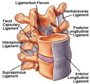
Figure 1: Spinal ligaments
From previous research we obtained formulae to deter-mine the change in subtended distances between two lines/curves, but the requirement was that the ini-tial line/curve on which the force is applied should be straight, and after deformation it is curved. In our study we have an initially curved rod. For this specific situ-ation we could not find any informsitu-ation or formulae for determining the change in subtended distance between two curves (starting with an initially curved rod. In the next section we derive a formula for this special case. The classical Euler buckling theory will also be used.
2
A formula to calculate the change
in subtended distance between two
curves
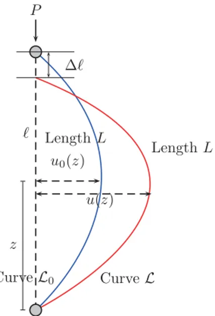
In this section we derive a formula to determine the change in distance between two curves, with the assump-tion and condiassump-tion that the lengths of the two curves re-main the same and equal, before and after deformation. The initial curve (before deformation), is described by the function u0(z). The deformed state of the curve is described by the functionu(z). (See Figure 2)
P
u(z) u0(z)
z
ℓ LengthL
LengthL
CurveL0 CurveL ∆ℓ
Figure 2: The buckling of an initially curved rod.
Consider the curves to be composed ofichords each with the same lengthLi, subtended byδi on thez-axis. (See Figure 3)
The lengths of the cordsLi remain the same after defor-mation.
Li
Li u0(z)
u(z)
α θ δ(δ(zi))
δ(zi)
Figure 3: Composed curved rod.
From simple trigonometry we know that
tanα = u′ 0(z) tan (α+θ) = u′
(z)
cosα = 1
1 + [u′ 0(z)]2
cos (α+θ) = 1
1 + [u′(z−δ(δz))]2. (1)
Another assumption we make is that the difference be-tween u′
(z−δ(δz)) and u′
(z) is negligibly small. That
means u′
(z−δ(δz)) ≈ u′
(z). From this we obtain an equation to determine the difference in the lengths sub-tending the initial chord and the deformed chord:
δz−δ(δz) = Lcos (α+θ)
= δz
cosαcos (α+θ)
δ(δz) = δz
1−
1 + [u′ 0(z)]2
1 + [u′(z−δ(δz))]2
(2)
Equation 2 holds for each chord i. Adding up all the smallδ(δzi) we find an expression for ∆ℓ:
∆ℓ = n
i=1 δ(δzi)
= n
i=1
1−
1 + [u′ 0(zi)]2 1 + [u′(zi)]2
δzi (3)
Using the limiting process, we obtain
l
0
1−
1 + [u′ 0(z)]2 1 + [u′(z)]2
dz (4)
3
Variational method
Having an expression for ∆l, our next step is to look at the classical Euler buckling theory, but we modify the theory to hold for an initially curved rod, since the human spine has an initial curvature. We apply the minimal potential approach on an initially curved rod, considering the spine as a whole.
In Figure 2P is the applied force (from the top);u(z) is the displacement; l is the length of the rod (the length remains the same); z represents the distance from the initial point andu0(z) is the initial displacement of the curved rod.
The bending moment for a straight rod that is buckled, is given by
M(z) =P u(z). (5)
The constitutive equation is given by
M(z) =−EId 2u
dz2 (6)
whereEI is the bending stiffness.
But the human back is not straight initially, and therefore we are considering an initially curved rod (see Figure 2). We consider the difference between the initial bending and the actual bending that occurred to obtain the actual bending. Therefore the actual bending is given by
u′′
(z)−u′′
and now the constitutive equation becomes
M(z) =−EI(u′′
(z)−u′′
0(z)). (8)
We rewrite the constitutive equation as
u′′
(z) +λ2u(z) =u′′
0(z) =P u(z) (9)
with
λ=
P
EI (10)
where we have the conditions:
u(0) =u(l) = 0. (11)
By definition, the potential energy in the deformed state of the material
U =W−A(ub) (12)
where U is the total potential energy, W is the elastic potential energy, and A(ub) refers to the work done by (given) external forces.
W =1 2EI
l
0 (u′′
(z)−u′′
0(z))2dz (13)
and
A(ub) = P∆l
= P
l
0 1−
1 + (u′ 0(z))2 1 + (u′(z))2 dz
Using Taylor series expansion and looking at the maxi-mum value for|u′
0(z)|and therefore max|tanθ|, assuming θ < 10◦
we can neglect all the fourth order and higher order terms. That gives us
A(b)
u ≈ P
⎡
⎣ℓ−
l
0
1 + 1 2((u
′
0(z))2−(u ′
(z))2)
⎤
⎦ dz
= −P
2
l
0 [(u′
0(z))2−(u ′
(z))2]dz (14)
Substituting (13) and (14) back into (12) we get an ex-pression for the potential energy
U = 1 2EI
l
0 (u′′
(z)−u′′
0(z))2dz
−1
2P l
0 [(u′
(z))2−(u′
0(z))2]dz
= U{u(z)}. (15)
For verification of the constitutive equation (9) we ob-tained, we now want to look at the effect that a small disturbanceδ will have on the potential function U(z). For this we consider the variation ofU andu
δU =U(u(z) +δu(z))−U(u(z)) (16)
where|δu(z)|is small, and δu(z) satisfies the kinematic boundary conditions
δu(0) =δu(l) = 0. (17)
By substituting (15) in (16) we obtain, after some calcu-lation,
δU(z) = EI l
0 (u′′
(z)−u′′ 0(z))
d2
dz2[δ(u(z))] dz
−P l
0
u′
(z)dδu(z) dz
dz. (18)
Using integration by parts with the constraints
u′′
(l)−u′′ 0(l) =u
′′
(0)−u′′
0(0) = 0. (19)
and the kinematic boundary conditions from (17) we ob-tain
δU = ℓ
0
EI(uiv(z)−u′′
0(z) +P u ′′
(z))
δ(u(z))dz
(20)
ButδU should be zero for allδu(z), because we are look-ing for an equilibrium stateu(z) which impliesδU = 0 This gives us the following equation and constraints
EIu(4)(z) +P u′′
(z) =EIu(4)0 (z)
subject to
EI[u′′
(0)−u′′
0(0)] =EI[u ′′
(l)−u′′
0(l)] = 0, u(0) =u0(0) =u(l) =u0(l) = 0.
Integrating the equation twice yields
EIu′′
(z) +P u(z) =EIu′′
0(z) +A1z+A2
but from our constraints we have that
A1=A2= 0.
Therefore
u′′
(z) +λ2u(z) =u′′
0(z) (21)
where
λ=
P EI.
Equation (21) is similar to (9), therefore we have a non-homogeneous linear equation.
In order to solve this differential equation we need an es-timation for the initial form of the spine. Looking at the literature we see a representation of the human spine in Figure 4.
Figure 4: A function describing the initial form of the human spine
Hereby we can describe the form of the spine by fitting a curve with optimization. The anterior (front), posterior and central line from a mathematical fitting is given in Figure 4 below. The equation describing the anterior, posterior and central line of the curved spine, is given by
x = 4 + 0.065y+ 11.7 sin(6πy
1320)−9.8 sin(2 6πy 1320)
+ −3 sin(36πy 1320)
(22)
where y, measured on a scale with the vertical distance form the top to the bottom of the curve given by the function, is 340 units, as seen on the right hand side of Figure 4.
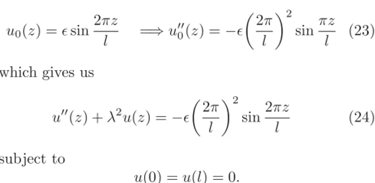
Keeping (22) in mind we choose our initial displacement
function to be
u0(z) =sin 2πz
l =⇒u ′′
0(z) =−
2π
l
2
sinπz l (23)
which gives us
u′′
(z) +λ2u(z) =−
2π l
2
sin2πz
l (24)
subject to
u(0) =u(l) = 0.
Solving this nonhomogeneous linear equation, we choose the particular solution to be
up(z) = csin2πz l
u′
p(z) = c
2π
l
cos2πz l
u′′
p(z) = −c
2π l
sin2πz l
Next we determine the constant c by substituting the particular solution back into the original problem:
−
2π
l
2
csin2πz l +λ
2csin2πz l =−
2π
l
2
sin2πz l
−
2π
l
2
+λ2
c=−
2π
l
2
Thus we have
c=
−
2π l
2
2π l
2
−1 +
l 2π
2
λ2
=
1−
lλ 2π
2
which gives a displacement function for the particular solution
up(z) = 1−
lλ 2π
2sin
2πz
l (25)
For the general homogeneous equation we have
uh(z) =Acosλz+Bsinλz
where A and B are constants to be determined. This gives us the displacement function for the nonhomoge-neous linear equation
u(z) = up(z) +uh(z)
=
1−
ℓλ 2π
2sin
2πz
l +Acosλz+Bsinλz
subject to
u(0) =u(l) = 0
and therefore it simplifies to
u(z) = 1− lλ 2π 2sin 2πz l (27) Let ℓλ 2π = ˆλ, then we have
u(z) = 1− lλ 2π 2sin 2πz l
Hence, we found a formula for the displacement function u(z).
4
Stability analysis
Our objective is to have a potential energy function in order to analyze the stability as stated earlier. We used the first condition for stability, that the first derivative of the potential function should be zero (mechanical equilib-rium), to derive the displacement function in (27). The initial displacement function as given by (23).
Next we look at the second condition for spinal stability, using the method of variation. We want to consider the effect that a small disturbanceδ will have on the poten-tial function U(z). For this we consider the variation of U and u, but now we develop our potential function U up to second order inδu:
U(u+δu) = U(u(z)) +EI ℓ
0 (u′′
(z)−u′′ 0(z))δu ′′ (z)dz −P ℓ 0 u′ (z)δu′ (z)dz +1 2EI ℓ 0 [δu′′
(z)]2−1
2P ℓ
0 [δu′
(z)]2dz
= U+δU +δ2U (28)
where |δu(z)|is small, and δu(z) satisfies the kinematic boundary conditions
δu(0) =δu(l) = 0. (29)
The equilibrium state is stable ifδ2U >0 for all admissi-bleδu(z), withδu(z)= 0. A complete representation for δu(z) is thus
δu(z) = ∞
k=1
aksin2kπz
ℓ (30)
whereak is arbitrary. Then
δ2U(u(z)) = 1 2EI ∞ k=1 ∞ m=1 ℓ 0 2kπ ℓ
22mπ
ℓ 2 sin 2kπ ℓ sin 2mπ ℓ − P EI 2kπ ℓ 2mπ ℓ cos 2kπ ℓ cos 2mπ ℓ dz (31)
Choosea1= 1, ak = 0, k≥2 which is the most unfavor-able situation. This yields
δ2U(u(z)) = 1 2 ℓ 0 2π ℓ 4
sin22πz ℓ − 2π ℓ 2 P EI
cos22πz ℓ dz = 1 2 2π ℓ 2 ℓ 2 2π ℓ 2
EI−P
(32)
Hence, for stability of the equilibrium state we have
δ2U(u(z))>0 ⇐⇒
2π
ℓ
2
EI−P >0
(33)
The conclusion from (33) is:
• for P < 2π ℓ 2 EI
the equilibrium state ofu(z) is stable
• for P > 2π ℓ 2 EI
5
Conclusions and future work
We obtained a sufficient result to draw conclusions from for the stability of the human spine. The relation between the force working on the spine (P) and the bending stiff-ness (EI) (see equation 33) can be tested by using data from the literature. This will be our next objective.
References
[1] Bergmark, A.1989. Stability of the lumbar spine. A study in mechanical engineering. Acta
orthopaed-ica Scandinavorthopaed-ica. Supplementum, 230:1–54.
[2] Nixon, J. and Brown, H.M.1986. Intervertebral disc mechanics: a review. Journal of the Royal
So-ciety of Medicine, 79:100–104.