www.geosci-model-dev.net/4/571/2011/ doi:10.5194/gmd-4-571-2011
© Author(s) 2011. CC Attribution 3.0 License.
Geoscientific
Model Development
Pliocene Model Intercomparison Project (PlioMIP): experimental
design and boundary conditions (Experiment 2)
A. M. Haywood1, H. J. Dowsett2, M. M. Robinson2, D. K. Stoll2, A. M. Dolan2, D. J. Lunt3, B. Otto-Bliesner4, and M. A. Chandler5,6
1School of Earth and Environment, University of Leeds, Woodhouse Lane, Leeds, LS2 9JT, UK
2Eastern Geology and Paleoclimate Science Center, U.S. Geological Survey, MS926A, 12201 Sunrise Valley Drive, Reston, VA 20192, USA
3School of Geographical Sciences, University of Bristol, University Road, Bristol, BS8 1SS, UK 4CCR, CGD/NCAR, P.O. Box 3000, Boulder, CO 80307-3000, USA
5Center for Climate Systems Research, Columbia University, 2880 Broadway, New York, NY, 10025, USA 6NASA Goddard Institute for Space Studies, New York, NY, USA
Received: 18 February 2011 – Published in Geosci. Model Dev. Discuss.: 2 March 2011 Revised: 27 June 2011 – Accepted: 1 July 2011 – Published: 1 July 2011
Abstract. The Palaeoclimate Modelling Intercomparison Project has expanded to include a model intercomparison for the mid-Pliocene warm period (3.29 to 2.97 million yr ago). This project is referred to as PlioMIP (the Pliocene Model In-tercomparison Project). Two experiments have been agreed upon and together compose the initial phase of PlioMIP. The first (Experiment 1) is being performed with atmosphere-only climate models. The second (Experiment 2) utilises fully coupled ocean-atmosphere climate models. Follow-ing on from the publication of the experimental design and boundary conditions for Experiment 1 in Geoscientific Model Development, this paper provides the necessary de-scription of differences and/or additions to the experimental design for Experiment 2.
1 Introduction
The mid-Pliocene warm period (mPWP) is defined by the United States Geological Survey’s PRISM Group (Pliocene Research Interpretation and Synoptic Mapping; http:// geology.er.usgs.gov/eespteam/prism/index.html) as the inter-val between 3.29 and 2.97 Ma (according to the geomagnetic polarity timescale of Berggren et al. 1995), lying between the transition of oxygen isotope stages M2/M1 and G19/G18 (Shackleton et al., 1995), in the middle part of the Gauss Nor-mal Polarity Chron (Dowsett et al., 1999). The “Time Slab”
Correspondence to:A. M. Haywood
represents a climatically distinct period during the Pliocene when Earth’s climate was, on the whole, warmer than present (Dowsett et al., 1999; Dowsett, 2007).
The mPWP has been the subject of intense study for the last two decades. There are many reasons for this, but an im-portant driver has been our desire to understand the dynamics of past warm climates as a potential guide to understanding climate change in the future (Haywood et al., 2009). The mPWP is well suited to this task. The climatic signal (change from modern) is sufficiently large, for many geographical re-gions, to be differentiated from the noise generated by the uncertainties and limitations inherent in the techniques used for palaeoclimatic/palaeoenvironmental reconstruction. The interval was the last time in Earth history when global tem-peratures were significantly warmer than modern, over a pe-riod longer than any Quaternary interglacial. It is unique in that continental configurations were relatively unchanged from today, and geological proxies are superior to those of preceding warm periods due to improved geographic cover-age, more reliable biota-environment correlations and higher resolution stratigraphy (Dowsett, 2007).
use versions of the US Geological Survey’s PRISM Group boundary condition data sets (e.g. Dowsett, 2007). This Spe-cial Issue ofGeoscientific Model Developmentrepresents the first set of co-ordinated publications from PlioMIP. It (a) de-scribes the chosen experimental design for Experiments 1 and 2, (b) includes a detailed description of the boundary conditions used in both experiments, and (c) presents con-tributions from each participating model group, describing how the boundary conditions were implemented into the dif-ferent climate models and the basic results from the exper-iments themselves. This detailed record for the rationale and specifics of the experimental design, construction of the boundary conditions data sets, and critically, how these were implemented into each climate model, will provide an invalu-able reference when the intercomparison phase of PlioMIP is reached. This will help the PlioMIP/PMIP community to un-derstand more easily the differences which will inevitably be observed between mid-Pliocene warm period (mPWP) sim-ulations. The purpose of this paper is to briefly describe the experimental design and boundary conditions for PlioMIP Experiment 2, focussing only on the aspects that differ from Experiment 1. Participating groups should refer to Haywood et al. (2010), for full details of Experiment 1 and for details relevant to Experiment 2 that are not repeated here.
2 Experimental Design – Experiment 2
2.1 Integration, atmospheric gases/aerosols, solar constant/orbital configuration
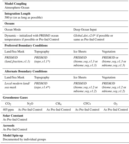
The experimental design for Experiment 2 is summarised in Table 1. The experiment integration length was set to 500 yr in accordance with CMIP5 guidelines (Coupled Model Inter-comparison Project Phase 5) for coupled model experiments (see: http://cmip-pcmdi.llnl.gov/cmip5/docs/Taylor CMIP5 design.pdf).
As in PlioMIP Experiment 1, the concentration of CO2 in the atmosphere was set to 405 ppmv. In the absence of any adequate proxy data, all other trace gases and aerosols were specified to be consistent with the individual group’s pre-industrial control experiments.
When trying to specify CO2 as far back in time as the Pliocene epoch uncertainty is inevitable. Evidence for Pliocene CO2comes from a number of sources: (1) the stom-atal density of fossil leaves (K¨urschner et al., 1996), (2) car-bon isotope analyses (e.g. Raymo et al., 1996), (3) alkenone-based estimates (Pagani et al., 2010; Seki et al., 2010) and (4) boron isotope analyses (e.g. Seki et al., 2010). The values of CO2from each of these proxies differ. However, within error they overlap. The stomatal density records support a CO2of 350 to 380 ppmv. The average of the Raymo carbon isotope analyses is similar to the stomatal-based estimates but peaks above that value (beyond 425 ppmv) occur and are entirely plausible. The Pagani et al. study looked at reconstructed
CO2from a number of different marine records and the work shows clearly that in three of the six marine records a CO2 value of 400 or 405 is perfectly reasonable and the CO2range stated by Pagani et al. (2010) is 365 to 415 ppmv. In the Seki et al. (2010) study the alkenone-based CO2 record is consistent with a value around 400 ppmv. The highest reso-lution section of the Seki et al. (2010) boron isotope record shows a decline in CO2from 400 to 280 after 3 million yr. Pliocene CO2is an important ongoing area of research with new records coming online in the next few years. Beyond Ex-periment 2, CO2is an obvious choice for sensitivity tests as part of PlioMIP and is one of the many justifications for util-ising coupled ocean-atmosphere models within the project.
The solar constant and orbital configuration was specified as the same as each participating group’s pre-industrial trol run. The PRISM data set of mid-Pliocene boundary con-ditions (Dowsett, 2007) represents an average of the warm intervals during the time slab (3.29 to 2.97 million yr) rather than a discrete time slice, making it challenging to prescribe an orbital configuration which is representative of the entire ∼300 000 yr interval. Furthermore, it is difficult to provide an average insolation forcing at the top of the atmosphere in some climate models, with some models requiring specific values for eccentricity, obliquity and precession. Therefore, PlioMIP decided to specify a modern orbital configuration, even though available astronomical solutions (e.g. Laskar et al., 2004) indicate that this may not provide the most rep-resentative mean orbital forcing for the mPWP (see Hay-wood et al., 2010). In the future this uncertainty can be ex-plored through sensitivity experiments in which the orbital configuration is changed and provides a further justification of the implementation of coupled-ocean atmosphere models in PlioMIP.
2.2 Adoption/availability of a “Preferred” and “Alternate” experimental design
Table 1.Experimental design – PlioMIP Experiment 2.
Model Coupling
Atmosphere-Ocean
Integration Length
500 yr (or as long as possible)
Oceans
Ocean Mode Deep Ocean Input
Dynamic – initialized with PRISM3 ocean Global dot v2.0* if possible or temperatures if possible or Pre-Ind Control same as Pre-Ind Control
Preferred Boundary Conditions
Land/Sea Mask Topography Ice Sheets Vegetation
PRISM3D PRISM3D PRISM3D PRISM3Dor
(land fraction v1.1) (topo v1.1*) (biome veg v1.3or (biome veg v1.3or
mbiome veg v1.3) mbiome veg v1.3)
Alternate Boundary Conditions
Land/Sea Mask Topography Ice Sheets Vegetation
Local modern land/ PRISM3D PRISM3D PRISM3D sea mask (topo v1.4*) (biome veg v1.2or (biome veg v1.2or
mbiome veg v1.2) mbiome veg v1.2)
Greenhouse Gases
CO2 N2O CH4 CFCs O3
405 ppm As Pre-Ind Control As Pre-Ind Control As Pre-Ind Control As Pre-Ind Control
Solar Constant
As Pre-Ind Control
Aerosols
As Pre-Ind Control
Model Spin-up
Documented by individual groups
∗Applied as an anomaly to control experiment data sets used by each participating group rather than as an absolute.
Those groups who are able to adopt the preferred exper-imental design will have to adjust the bathymetry of the deglaciated West Antarctic region. To avoid numerical in-stabilities groups will specify a flat bathymetry with an aver-age depth of 500 m. This bathymetry will be graded into the modern bathymetry. For those models which are very sen-sitive to bathymetric alteration, groups are free to do what is necessary to enable a simulation to be successfully com-pleted.
Given the absence of a global data set for mPWP bathymetry in all other regions ocean bathymetry will be specified as modern. However, there has been a discussion recently regarding the depth of potentially critical sills in the North Atlantic (e.g. Jones et al., 2002). Robinson et al. (2011) have shown that the exact depth of the
Greenland-Scotland Ridge specified in coupled climate models can have a significant effect on model predictions of North At-lantic Deepwater formation (NADW), thermohaline circula-tion (THC) and increased SSTs in the North Atlantic and Arctic. Investigation of such uncertainties is beyond the scope of the first phase of PlioMIP but could become a fo-cus for sensitivity tests in the future.
2.3 Implementation of ocean temperatures and topography as an anomaly
conditions, it was decided to implement both the Pliocene topography and initial sea surface temperatures (SST) (from Experiment 1) and SST and deep ocean temperatures (from Experiment 2) as an anomaly to the standard modern ocean temperature and topographic data set used by each modelling group’s individual model. For Experiment 2 to create the initial Pliocene ocean temperature and topography, the dif-ference between the PRISM Pliocene and PRISM Modern ocean temperatures and topography will be calculated and added to the modern ocean temperature and topographic data sets each participating modelling group employs.
In other words:
Topo Plio=(Topo Plio PRISM3D (1)
−Topo Modern PRISM3D) +Topo Modern Local and
OceanT Plio=(OceanT Plio PRISM3D (2) −OceanT Modern PRISM3D)
+OceanT Modern Local
However, when using such a method, a potential mis-match between mid-Pliocene and modern topography land-sea masks is possible. This will be overcome by using abso-lute Pliocene topography and ocean temperatures in regions where no modern data are given (such as for the Pliocene topography in the Hudson Bay region). Modern SSTs are projected on the same Pliocene grids (preferred and alter-nate) to make anomalies easier to generate. There may be mismatches (for example in the West Antarctic region) be-tween the Pliocene deep ocean temperature data, where it is provided, and the Pliocene land/sea mask. Where this is the case,Global dot v2.0deep ocean temperatures should be ex-trapolated horizontally into regions with no data coverage, therefore maintaining theGlobal dot v2.0vertical ture profile. Groups unable to alter the initial ocean tempera-ture state should begin the simulation with a modern control state and document the spin-up of the simulation. Salinity should be derived from Levitus and Boyer (1994) or an ex-isting modern (control) simulation. The starting atmospheric conditions for Experiment 2 should be derived from the end of Experiment 1 if possible.
3 Description of Boundary Conditions (PRISM3D)
A full description of the mPWP land-sea mask (including the nature of ocean gateways) and topography (outside of ice sheet regions), ice sheet height and extent, SST (see Fig. 1), sea-ice extent, vegetation type and distribution, soils, lakes and river routing is provided in Haywood et al. (2010; this volume). Here it is only necessary to describe the construc-tion and nature of the three-dimensional data set for ocean temperatures that groups have the option of using to initialise their ocean models for PlioMIP Experiment 2.
3.1 The PRISM3D data set of ocean temperatures
The PRISM3D deep ocean temperature reconstruction (Fig. 2) is presented at a 4◦
latitude by 5◦
longitude reso-lution with 33 depth layers, based upon 27 localities, un-evenly distributed among the ocean basins. While not op-timal for generating a global reconstruction, this represents possibly the largest number of temperature estimates for any deep-water reconstruction from any time interval. Spe-cific steps in the reconstruction methodology are listed in Dowsett et al. (2009) Supplement A (http://www.clim-past. net/5/769/2009/cp-5-769-2009-supplement.pdf). Because the PRISM3D reconstruction is designed for coupled ocean-atmosphere general circulation models, it represents a recon-struction of a prescribed day, arbitrarily chosen to be 1 De-cember (this does not imply that climate models must be in-tegrated from this date). The PRISM3D November and De-cember monthly SST reconstructions were averaged to ap-proximate the SST for mid-Pliocene 1 December. A surface-temperature anomaly was created by subtracting the modern 1 December SST field (Reynolds and Smith, 1995) from the Pliocene 1 December data. The surface temperature anomaly was then added to the 0 m layer of Levitus and Boyer (1994) (converted to a 4◦×
5◦
resolution) to create the PRISM3D 0 m reconstruction. Since no data points fall between 0 m and 1100 m in the deep ocean temperature data set, PRISM chose to use a mathematical function that decreases the weight of the surface anomaly with depth down to 1400 m (see Dowsett et al., 2009). Between 900 m and 1400 m that anomaly was further modified based upon data from Southern Ocean sites to accomplish an adjustment or vertical expansion of palaeo Antarctic Intermediate Water (AAIW).
In the Atlantic sector of the Southern Ocean, data suggest warmer palaeo NADW expansion in the region relative to modern day (Dowsett et al., 2009). Warm anomalies for the mid-Pliocene at all sites are in keeping with the hypothesized warmer and stronger flux ofpalaeoNADW and diminished (colder) palaeo Antarctic Bottom Water production relative to today. In the western Pacific, sites that monitor Pacific Deep Water today show small positive anomalies for the mid-Pliocene. PRISM interprets these data to indicate the overall warmer conditions of the water masses that mixed to form
palaeoPDW. In the eastern Pacific, temperature data can be explained by a vertical displacement of AAIW concomitant with overall warming of PDW.
A complete discussion of the rationale and methodology used for the PRISM Deep Ocean Temperature reconstruction can be found in Dowsett et al. (2009).
4 Data management and planned analyses
Fig. 1. PRISM3D SST anomaly for February (top left) and August (top right). PRISM3D sea-ice extent for February (bottom left) and August (bottom right).
Fig. 2. Longitudinal profiles of ocean temperature from transects at(a)15◦W,(b)45◦W,(c)90◦W and(d)165◦E. All temperatures are
shown in◦C. Contour interval is 2◦C. Black contour lines show modern temperature overlaid on coloured regions showing the mid-Pliocene
and stored within the PMIP2 database. Specifically, for PlioMIP Experiment 1, this refers to PMIP2 rec-ommended outputs for the atmosphere (outlined on the PMIP2 website http://pmip2.lsce.ipsl.fr/>Experimental Design>Variables>Atmosphere). PMIP/PlioMIP requires participants to prepare their data files so that they meet the following constraints (regardless of the way their models pro-duce and store their results).
– The data files have to be in the (now widely used) netCDF binary file format and conform to the CF (Cli-mate and Forecast) metadata convention (outlined on the website http://cf-pcmdi.llnl.gov/).
– There must be only one output variable per file. – For the data that are a function of longitude and
lati-tude, only regular grids (grids representable as a Carte-sian product of longitude and latitude axes) are allowed. – The file names have to follow the PMIP2 file name
con-vention and be unique.
Participants are encouraged to create the files for submis-sion to the database using the CMOR (Climate Model Output Rewriter) library. This library has been specially developed to help meet the requirements of the Model Intercompari-son Projects. Details of the CMOR library are provided on the PMIP2 website (http://pmip2.lsce.ipsl.fr/>Experimental design> Output format>CMOR library). Proposals for model analyses using PlioMIP Experiment 1 data can be made using the established protocols outlined on the PlioMIP website.
5 Conclusions
This paper provides a model intercomparison project de-scription for the Pliocene Model Intercomparison Project (PlioMIP) and documents in detail the experimental design. Specifically, this paper describes the experimental design and boundary conditions utilised for Experiment 2 of PlioMIP, following a companion paper for Experiment 1. Experi-ment 2 will utilise coupled ocean-atmosphere models and will enable the sensitivity of the simulated coupled ocean-atmosphere system in a palaeoclimate context to be explored. It also provides the necessary foundation for further sensitiv-ity tests as part of PlioMIP that will explore uncertainties in-troduced in the climate modelling from specified trace gases and orbital configurations etc.
Supplementary material related to this article is available online at:
http://www.geosci-model-dev.net/4/571/2011/ gmd-4-571-2011-supplement.zip.
Acknowledgements. This work is a product of the US Geological Survey PRISM (Pliocene Research, Interpretation and Synop-tic Mapping) Project and the Pliocene Model Intercomparison Project (PlioMIP), which is part of the international Palaeoclimate Modelling Intercomparison Project (PMIP). HD and MR thank the USGS Office of Global Change for their support. AH and DL acknowledge the UK Natural Environment Research Coun-cil for funding the UK contribution to PlioMIP (NERC Grant NE/G009112/1). AH acknowledges the Leverhulme Trust for their support through the award of a Philip Leverhulme Prize as well as the European Research Council for the provision of a Starting Grant (ERC StG 278636: Plio-ESS).
Edited by: J. C. Hargreaves
References
Berggren, W. A., Kent, D. V., Swisher, C. C., and Aubry, M. P.: A revised Cenozoic geochronology and chronostratigraphy, in: Geochronology, time scales and global stratigraphic correlation, edited by: Berggren, W. A., Kent, D. V., Aubry, M. P., and Hard-enbol, J., Tulsa, Soc. Sed. Geol., Spec. Pub. 54, 129–212, 1995. Braconnot, P., Otto-Bliesner, B., Harrison, S., Joussaume, S.,
Pe-terchmitt, J.-Y., Abe-Ouchi, A., Crucifix, M., Driesschaert, E., Fichefet, Th., Hewitt, C. D., Kageyama, M., Kitoh, A., Lan, A., Loutre, M.-F., Marti, O., Merkel, U., Ramstein, G., Valdes, P., Weber, S. L., Yu, Y., and Zhao, Y.: Results of PMIP2 coupled simulations of the Mid-Holocene and Last Glacial Maximum – Part 1: experiments and large-scale features, Clim. Past, 3, 261– 277, doi:10.5194/cp-3-261-2007, 2007a.
Braconnot, P., Otto-Bliesner, B., Harrison, S., Joussaume, S., Pe-terchmitt, J.-Y., Abe-Ouchi, A., Crucifix, M., Driesschaert, E., Fichefet, Th., Hewitt, C. D., Kageyama, M., Kitoh, A., Loutre, M.-F., Marti, O., Merkel, U., Ramstein, G., Valdes, P., Weber, L., Yu, Y., and Zhao, Y.: Results of PMIP2 coupled simula-tions of the Mid-Holocene and Last Glacial Maximum – Part 2: feedbacks with emphasis on the location of the ITCZ and mid- and high latitudes heat budget, Clim. Past, 3, 279–296, doi:10.5194/cp-3-279-2007, 2007b.
Dowsett, H. J.: The PRISM palaeoclimate reconstruction and Pliocene sea-surface temperature, edited by: Williams, M., Hay-wood, A. M., Gregory, J., and Schmidt, D. N., in: Deep-time perspectives on climate change: Marrying the signal from computer models and biological proxies, Micropalaeontological Soc., Spec. Pub., Geol. Soc. of London, London, UK, 459–480, 2007.
Dowsett, H. J., Barron, J. A., Poore, R. Z., Thompson, R. S., Cronin, T. M., Ishman, S. E., and Willard, D. A.: Middle Pliocene pa-leoenvironmental reconstruction: PRISM 2, U.S. Geol. Surv., Open File Rep., 99–535, 1999.
Dowsett, H. J., Robinson, M. M., and Foley, K. M.: Pliocene three-dimensional global ocean temperature reconstruction, Clim. Past, 5, 769–783, doi:10.5194/cp-5-769-2009, 2009.
Haywood, A. M., Dowsett, H. J., Otto-Bliesner, B., Chandler, M. A., Dolan, A. M., Hill, D. J., Lunt, D. J., Robinson, M. M., Rosenbloom, N., Salzmann, U., and Sohl, L. E.: Pliocene Model Intercomparison Project (PlioMIP): experimental design and boundary conditions (Experiment 1), Geosci. Model Dev., 3, 227–242, doi:10.5194/gmd-3-227-2010, 2010.
Jones, S. M., White, N., and Maclennan, J.: V-shaped ridges around Iceland: implications for spatial and temporal patterns of mantle convection, Geochem. Geophy. Geosy., 3, 1059, doi:101029/2002GC000361, 2002.
K¨urschner, W. M., Van der Burgh, J., Visscher, H., and Dilcher, D. L.: Oak leaves as biosensors of late Neogene and early Pleis-tocene paleoatmospheric CO2concentrations, Mar. Micropale-ontol., 27, (1/4), 299–312, 1996.
Laskar, J., Robutel, P., Joutel, F., Gastineau, M., Correia, A. C. M., and Levrard, B.: A long term numerical solution for the insola-tion quantities of the Earth. Astron. Astrophys., 428, 261–285, doi:10.1051/0004-6361:20041335, 2004.
Levitus, S. and Boyer, T. P.: World Ocean Atlas 1994, Volume 2: Oxygen. NOAA Atlas NESDIS 2. U.S. Department of Com-merce, NOAA, NESDIS, 1994.
Pagani, M., Liu, Z., LaRiviere, J., and Ravelo, A. C.: High Earth-system climate sensitivity determined from Pliocene car-bon dioxide concentrations, Nature Geosci., 3, 27–30, 2010. Raymo, M. E., Grant, B., Horowitz, M., and Rau, G. H.:
Mid-Pliocene warmth: Stronger greenhouse and stronger con-veyor, Mar. Micropaleontol., 27, 313–326, doi:10.1016/0377-8398(95)00048-8, 1996.
Reynolds, R. W. and Smith, T. M.: A high-resolution global sea sur-face temperature climatology, J. Climate, 8, 1571–1583, 1995. Robinson, M. M., Valdes, P. J., Haywood, A. M., Dowsett,
H. J. Hill, D. J., and Jones, S. M.: Bathymetric con-trols on Pliocene North Atlantic and Arctic sea surface tem-perature and deepwater production, Palaeogeogr. Palaeocl., doi:10.1016/j.palaeo.2011.01.004, in press, 2011.
Seki, O, Foster, G. L., Schmidt, D. N., Mackensen, A., Kawamura, K., and Pancost, R. D.: Alkenone and boron-based Pliocene pCO2 records, Earth Planet. Sci. Lett., 292, (1–2), 201–211, 2010.