Large-scale features of Pliocene climate: results from the Pliocene Model Intercomparison Project

(1)

CPD

8, 2969–3013, 2012

Results from the Pliocene Model Intercomparison

Project

A. M. Haywood et al.

Title Page

Abstract Introduction

Conclusions References

Tables Figures

◭ ◮

Back Close

Full Screen / Esc

Printer-friendly Version

Interactive Discussion

Discussion

P

a

per

|

Dis

cussion

P

a

per

|

Discussion

P

a

per

|

Discussio

n

P

a

per

|

Clim. Past Discuss., 8, 2969–3013, 2012 www.clim-past-discuss.net/8/2969/2012/ doi:10.5194/cpd-8-2969-2012

Climate of the Past Discussions

This discussion paper is/has been under review for the journal Climate of the Past (CP). Please refer to the corresponding final paper in CP if available.

Large-scale features of Pliocene climate:

results from the Pliocene Model

Intercomparison Project

A. M. Haywood1, D. J. Hill1,2, A. M. Dolan1, B. Otto-Bliesner3, F. Bragg4,

W.-L. Chan5, M. A. Chandler6, C. Contoux7,8, A. Jost8, Y. Kamae9, G. Lohmann10, D. J. Lunt4, A. Abe-Ouchi5,11, S. J. Pickering1, G. Ramstein7, N. A. Rosenbloom3, L. Sohl6, C. Stepanek10, Q. Yan12, H. Ueda9, and Z. Zhang12,13

1

School of Earth and Environment, Earth and Environment Building, University of Leeds, Woodhouse Lane, Leeds, LS2 9JT, UK

2

British Geological Survey, Keyworth, Nottingham, UK

3

National Center for Atmospheric Research, Boulder, CO, USA

4

School of Geographical Sciences, University of Bristol, University Road, Bristol, BS8 1SS, UK

5

Atmosphere and Ocean Research Institute, University of Tokyo, Kashiwa, Japan

6

Columbia University – NASA/GISS, New York, NY, USA

7

Laboratoire des Sciences du Climat et de l’Environnement, Saclay, France

8

Unit ´e Mixte de Recherche 7619 SISYPHE, Universit ´e Pierre-et-Marie Curie Paris VI, Paris, France

9

Graduate School of Life and Environmental Sciences, University of Tsukuba, Tsukuba, Japan

10

(2)

CPD

8, 2969–3013, 2012

Project

Title Page

Tables Figures

◭ ◮

Back Close

Full Screen / Esc

Discussion

P

a

per

|

Dis

cussion

P

a

per

|

Discussion

P

a

per

|

Discussio

n

P

a

per

11

Research Institute for Global Change, JAMSTEC, Yokohama, Japan

12

Institute of Atmospheric Physics, Chinese Academy of Sciences, Beijing, China

13

Bjerknes Centre for Climate Research, Bergen, Norway

Received: 6 July 2012 – Accepted: 11 July 2012 – Published: 30 July 2012 Correspondence to: A. M. Haywood (earamh@leeds.ac.uk)

(3)

CPD

8, 2969–3013, 2012

Project

Title Page

Tables Figures

◭ ◮

Back Close

Full Screen / Esc

Discussion

P

a

per

|

Dis

cussion

P

a

per

|

Discussion

P

a

per

|

Discussio

n

P

a

per

|

Abstract

Climate and environments of the mid-Pliocene Warm Period (3.264 to 3.025 Ma) have been extensively studied. Whilst numerical models have shed light on the nature of climate at the time, uncertainties in their predictions have not been systematically ex-amined. The Pliocene Model Intercomparison Project quantifies uncertainties in model

5

outputs through a co-ordinated multi-model and multi-model/data intercomparison. Whilst commonalities in model outputs for the Pliocene are evident, we show substan-tial variation in the sensitivity of models to the implementation of Pliocene boundary conditions. Models appear able to reproduce many regional changes in temperature reconstructed from geological proxies. However, data/model comparison highlights the

10

potential for models to underestimate polar amplification. To assert this conclusion with greater confidence, limitations in the time-averaged proxy data currently available must be addressed. Sensitivity tests exploring the “known unknowns” in modelling Pliocene climate specifically relevant to the high-latitudes are also essential (e.g. palaeogeog-raphy, gateways, orbital forcing and trace gasses). Estimates of longer-term sensitivity

15

to CO2 (also known as Earth System Sensitivity; ESS), suggest that ESS is greater

than Climate Sensitivity (CS), and that the ratio of ESS to CS is between 1 and 2, with a best estimate of 1.5.

1 Introduction

1.1 The mid-Pliocene warm period

20

(4)

CPD

8, 2969–3013, 2012

Project

Title Page

Tables Figures

◭ ◮

Back Close

Full Screen / Esc

Discussion

P

a

per

|

Dis

cussion

P

a

per

|

Discussion

P

a

per

|

Discussio

n

P

a

per

Both geological data and climate model outputs have shed light on the nature of mid-Pliocene climate and environments. During warm phases of the mid-Pliocene, highlighted by negative excursions inδ18O from benthic foraminifera, Antarctic and/or Greenland ice volume may have been reduced compared to modern (Lunt et al., 2008; Hill et al., 2010; Naish et al., 2009; Pollard and DeConto, 2009; Dolan et al., 2011), and

5

between 2.7 and 3.2 Ma BP peak sea-level is estimated to have been 22±10 m higher

than modern (Dowsett and Cronin, 1990; Miller et al., 2012). Sea surface temperatures (SSTs) were warmer than present-day (Dowsett et al., 2010), particularly in the higher latitudes and upwelling zones (e.g. Dekens et al., 2007; Dowsett et al., 2012). Sea-ice cover also declined substantially (e.g. Cronin et al., 1993; Polyak et al., 2010; Moran

10

et al., 2006). On land, the global extent of arid deserts decreased, and forests replaced tundra in the Northern Hemisphere (e.g. Salzmann et al., 2008). On the basis of climate model outputs, the global annual mean temperature may have increased by more than 3◦_{C (e.g. Haywood and Valdes, 2004). Meridional and zonal temperature gradients} were reduced, which had a significant impact on the Hadley and Walker circulations

15

(e.g. Contoux et al., 2012; Haywood et al., 2000; Kamae et al., 2011). The East Asian summer monsoon, as well as other monsoon systems, may have been enhanced (e.g. Wan et al., 2010).

Given the abundance of proxy data, the mPWP has become a focus for data/model comparisons that attempt to analyse the ability of climate models to reproduce a warm

20

climate state in Earth history (e.g. Haywood and Valdes, 2004; Salzmann et al, 2008; Dowsett et al., 2011, 2012). Furthermore, the mPWP has been proposed as an impor-tant interval to assess the sensitivity of climate to near current concentrations of carbon dioxide (CO2) in the long term (hundreds to thousands of years; Lunt et al., 2010).

1.2 Assessing uncertainty in models

25

(5)

CPD

8, 2969–3013, 2012

Project

Title Page

Tables Figures

◭ ◮

Back Close

Full Screen / Esc

Discussion

P

a

per

|

Dis

cussion

P

a

per

|

Discussion

P

a

per

|

Discussio

n

P

a

per

|

Haywood et al., 2000, 2009), there are likely to be significant differences in the details of their simulations, particularly regionally (Haywood et al., 2009). Inconsistencies are to be expected due to structural differences in models, and from differences in experi-mental design. The exploration of uncertainty in model simulations of past climate has taken three primary forms. The first two include the use of a single model to either

per-5

form boundary condition sensitivity experiments (e.g. Haywood et al., 2007; Lunt et al., 2012; Robinson et al., 2011; Dolan et al., 2011), or to perform a perturbed physics ensemble (e.g PalaeoQUMP and Plio-QUMP; e.g. Pope et al., 2011). The third method uses a standardised experimental design in an ensemble composed of different climate models (a multi-model ensemble; e.g. Braconnot et al., 2007).

10

The Palaeoclimate Modelling Intercomparison Project (PMIP) was initiated in 1991 to co-ordinate the systematic study of climate models, and to assess their ability to simu-late past climates (e.g. Joussaume and Taylor, 1995; Bracannot et al., 2012). PMIP also encourages the preparation of global reconstructions of palaeoclimates that can be used to evaluate climate models (e.g. Prentice and Webb, 1998). The focus of the

stud-15

ies carried out by PMIP has, until recently, been largely focussed on the Last Glacial Maximum and the mid-Holocene. However, in 2008 the Pliocene Modelling Intercom-parison Project (PlioMIP) was added as a component of PMIP. Previously, there had only been limited efforts in documenting differences in model simulations of the mPWP. For example, Haywood et al. (2000) attempted a model intercomparison between

ver-20

sions of the Hadley Centre for Climate Prediction and Research, the Goddard Institute for Space Studies (GISS) and National Center for Atmospheric Research (NCAR) cli-mate models. This comparison was hampered by the fact that the experimental design in each of these studies was not the same.

Haywood et al. (2009) compared the outputs from two mPWP experiments using

ver-25

(6)

CPD

8, 2969–3013, 2012

Project

Title Page

Tables Figures

◭ ◮

Back Close

Full Screen / Esc

Discussion

P

a

per

|

Dis

cussion

P

a

per

|

Discussion

P

a

per

|

Discussio

n

P

a

per

the Arctic). Terrestrial data/model comparison (DMC) indicated that HadAM3 provided a closer fit to proxy data (biome distributions) in the mid to high-latitudes. However, GCMAM3 performed better than HadAM3 in the tropics.

Whilst the scope of the model intercomparison presented in Haywood et al. (2009) was limited, it served to encourage the palaeoclimate modelling community to establish

5

a larger model intercomparison project (PlioMIP). Here we present an initial model in-tercomparison focussed on the large-scale features of mPWP climate derived from the PlioMIP ensemble. PlioMIP established the design for two initial experiments. Experi-ment 1 used atmosphere-only climate models (AGCMs). ExperiExperi-ment 2 utilised coupled atmosphere-ocean climate models (AOGCMs) where SSTs and sea-ice were predicted

10

variables. Here, we focus on the presentation of the “large scale features” of Pliocene climate, that is, global annual mean surface air temperature response (difference from the pre-industrial) in Experiment 1 and 2, zonal patterns of temperature and precip-itation change, polar amplification, comparisons of model results to proxy data, and finally implications for longer-term climate sensitivity as defined by Lunt et al. (2010;

15

Earth System Sensitivity).

2 Boundary conditions and experimental design

2.1 Participating modelling groups

Details of participating groups and models, and which experiment each group per-formed (Experiment 1 or 2 or both), can be found in Table 1. For Experiment 1 seven

20

modelling groups completed and submitted data from their model integrations. For Ex-periment 2 eight modelling groups completed and submitted data. The models used in both Experiment 1 and 2 sample differing levels of complexity and resolution from higher resolution IPCC AR5-class models, to intermediate resolution models. Details of boundary conditions and their implementation in each model, as well as the

ba-25

(7)

CPD

8, 2969–3013, 2012

Project

Title Page

Tables Figures

◭ ◮

Back Close

Full Screen / Esc

Discussion

P

a

per

|

Dis

cussion

P

a

per

|

Discussion

P

a

per

|

Discussio

n

P

a

per

|

Table 1 and in a PlioMIP special edition of the Journal Geoscientific Model Develop-ment (http://www.geosci-model-dev.net/special issue5.html).

2.2 Boundary conditions

Full details of the boundary conditions used for PlioMIP Experiments 1 and 2 are pro-vided in Haywood et al. (2010, 2011), respectively. In brief, both experiments utilised

5

the US Geological Survey PRISM3D boundary condition data set (Dowsett et al., 2010). For Experiment 1, this included information on monthly SSTs and sea-ice distri-butions, vegetation cover, sea-level, ice-sheet extent and topography. Given the chal-lenging nature of changing the land/sea mask in some atmosphere-ocean climate mod-els, two versions of the boundary conditions were provided for both Experiment 1 and 2.

10

The preferred data set included a change in the land/sea mask accommodating the re-moval of the West Antarctic Ice Sheet (WAIS), an increase in sea-level of 25 m, and the infilling of the Hudson Bay. The alternate data set specified no changes in the land/sea mask (although some groups did infill the Hudson Bay) but did remove the WAIS as far as possible by reducing topography down to sea-level and specifying tundra

veg-15

etation. NetCDF versions of all boundary conditions used for PlioMIP Experiment 1 and 2, along with guidance notes for boundary condition implementation can be found at http://geology.er.usgs.gov/eespteam/prism/prism pliomip data.html. They have also been uploaded as Supplement to Haywood et al. (2011).

In both Pliocene experiments the atmospheric concentration of carbon dioxide (CO2)

20

(8)

CPD

8, 2969–3013, 2012

Project

Title Page

Tables Figures

◭ ◮

Back Close

Full Screen / Esc

Discussion

P

a

per

|

Dis

cussion

P

a

per

|

Discussion

P

a

per

|

Discussio

n

P

a

per

2.3 Experimental design

The design of control runs and Pliocene Experiments 1 and 2 is outlined in Hay-wood et al. (2010) and HayHay-wood et al. (2011), respectively. Each group used their local/standard pre-industrial simulations as a control run. A 50 yr integration length was specified as a minimum for Experiment 1, with the final 30 yr used to

cal-5

culate the required climatological means. A minimum integration length of 500 yr was specified for Experiment 2, which is long enough to allow at least the sur-face climatology and oceans to intermediate depth to reach an equilibrium condi-tion. Again the final 30 yr were used to calculate climatological means. Required fields and data formats that all groups were asked to provide can be found at

10

http://geology.er.usgs.gov/eespteam/prism/prism pliomeet11.html.

For Experiment 2 modelling groups were given the choice of how to initialise their ocean model for the mPWP. They could spin up their model from a standard pre-industrial control run, or specify the PRISM3D data set of ocean temperatures (Dowsett et al., 2009).

15

3 Results: PlioMIP Experiments 1 and 2

3.1 Global annual mean temperature change and hydrological response

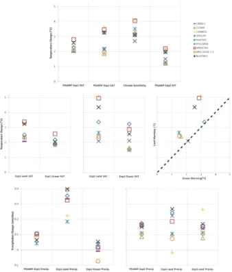
For the Experiment 1 ensemble, a range of global annual mean SAT anomalies from 1.75 to 2.55◦C is simulated, while in Experiment 2, the ensemble range is between 1.84 and 3.60◦C. No direct relationship between the magnitude of Pliocene SAT anomaly

20

and Climate Sensitivity is seen, demonstrating the importance of long-term climate drivers in mid-Pliocene warming. However, we note that MIROC4m and the COSMOS models have the two highest global annual SAT anomalies, as well as the highest published Climate Sensitivity estimates, showing CO₂and fast feedbacks to be among the primary drivers. As expected SAT anomalies over land (2.1 to 5.1◦C) are greater,

(9)

CPD

8, 2969–3013, 2012

Project

Title Page

Tables Figures

◭ ◮

Back Close

Full Screen / Esc

Discussion

P

a

per

|

Dis

cussion

P

a

per

|

Discussion

P

a

per

|

Discussio

n

P

a

per

|

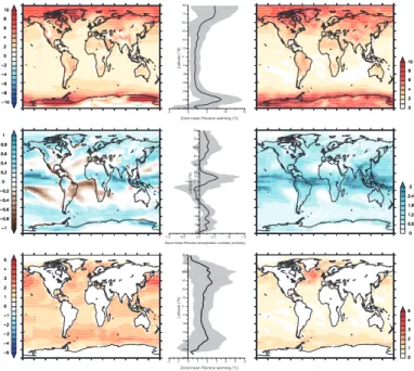
and show a larger spread of response than either SATs over the oceans or SSTs. SATs over the oceans increase by 1.5 to 3.2◦C and SSTs increase by 1.1 to 2.2◦C (Fig. 1). The greater SAT response over oceans, versus the SST response, is driven by changes at high latitudes where sea-ice is present in the control simulation but absent in the Pliocene simulation.

5

For Experiment 1, global annual mean precipitation rates increase by 0.04 to 0.11 mm day−1 (Fig. 1). The changes in global precipitation in Experiment 1 are dom-inated by the increases over the land, whereas the specified increases in SSTs are associated with very little increase in precipitation over the ocean. In Experiment 2, precipitation rates increase further to∼0.07 to 0.18 mm day−1. MIROC4m, COSMOS

10

and HadCM3 simulate the largest changes in total precipitation rate in the ensemble. A much smaller contrast is seen between increases on the land and over the ocean, although the partitioning of this increase is highly variable from model to model (Fig. 1).

3.2 Multi-model mean surface air temperature and precipitation (Experiment 1)

To facilitate the production of annual multi-model mean (MMM) SAT and precipitation

15

rate anomalies (Experiment 1 and 2), each participating models’ mPWP simulation was differenced to its respective pre-industrial control experiment. These data were then re-gridded on to the regular 2◦

×2◦ latitude/longitude grid of the PRISM3D boundary

conditions. MMM fields were then calculated as a simple mean of each of the individual model experiments. This allows us to evaluate the ensemble as a whole, without

down-20

weighting any of the individual models. Future work may include evaluation of each individual model against mPWP data and the production of weighted MMM, to improve estimates of mPWP climate. Individual model anomalies for SAT and total precipitation rate on their common/local grids are included in Supplement (Figs. S1 and S2).

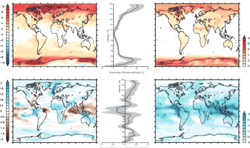
The Experiment 1 MMM SAT anomaly (Fig. 2) from pre-industrial is strongly

con-25

(10)

CPD

8, 2969–3013, 2012

Project

Title Page

Tables Figures

◭ ◮

Back Close

Full Screen / Esc

Discussion

P

a

per

|

Dis

cussion

P

a

per

|

Discussion

P

a

per

|

Discussio

n

P

a

per

Between 15◦ _{and 90}◦ _{north and south of the Equator the SAT anomaly becomes} pro-gressively stronger particularly over Greenland and the Arctic Basin, and in areas of West and East Antarctica. The zonal MMM SAT anomaly shows little or no change in the tropics and a clear polar amplification of temperatures. Temperatures increase by>10◦C in the Arctic and up to 20◦C in the Antarctic (Fig. 2). Over the oceans the

5

models’ SATs do not vary significantly from one another due to SSTs being prescribed. A 2σ of 1 to 4◦_{C is common in the MMM over land (Fig. 2). In regions dominated} by ice sheets or sea-ice the 2σ increases to 6 to 8◦C. In the same regions where the land/sea mask was altered (i.e. West Antarctica, the margins of East Antarctica and the Hudson Bay), the 2σ exceeds 8◦_{C. Such high inter-model di}

fferences are

10

attributable to the application of either the PlioMIP preferred or alternate experimental design (Haywood et al., 2010, 2011).

For total precipitation rate, the MMM indicates a complex response in the tropics (Fig. 2). In the Central and Western Pacific, precipitation rates near the Equator are reduced by ∼1 mm day−1. At 15◦ north and south of the Equator, and in the

East-15

ern Equatorial Pacific, precipitation rates increase by more than 2 mm day−1_{. Over the} African continent and the Indian sub-continent precipitation rates generally increase (0.1 to ∼2 mm day−1). Over the majority of the Indian Ocean precipitation rates are

reduced. Over North America precipitation rates increase in the north-west and are reduced in the south-west. Over ice-free regions of Greenland and Antarctica

precip-20

itation rates increase. Finally, large increases in precipitation rate (>2 mm day−1) are predicted in the Northern North Atlantic and the Nordic Seas.

Such regional differences are reproduced in the zonal MMM precipitation anomaly (Fig. 2). Around the Equator, precipitation rates decrease by∼0.4 mm day−1. 15◦north

and south of the Equator precipitation rates increase by up to 0.3 mm day−1. The zonal

25

(11)

CPD

8, 2969–3013, 2012

Project

Title Page

Tables Figures

◭ ◮

Back Close

Full Screen / Esc

Discussion

P

a

per

|

Dis

cussion

P

a

per

|

Discussion

P

a

per

|

Discussio

n

P

a

per

|

ensemble can exceed 3 mm day−1, whereas in most other areas the 2σ is no greater than 1.5 mm day−1(Fig. 2).

3.3 Multi-model mean surface air/sea surface temperature/precipitation (Experiment 2)

The process for constructing annual MMMs for Experiment 2 was the same as that

5

adopted for Experiment 1, except for the inclusion of SSTs. Individual model anomalies for SAT, total precipitation rate and SSTs on their common/local grids are included in the Supplement (Figs. S3–S5). In the tropics, the MMM indicates a general pattern of SAT warming of 1 to 2◦C over the oceans (Fig. 3). In the same region, warming over the land ranges from 1 to 6◦_{C. From the mid to high latitudes a pattern of progressively}

10

larger SAT anomalies is predicted reaching a maximum change over Greenland and the Arctic, West Antarctica and areas of East Antarctica. The zonal mean SAT anomaly displays∼2◦C warming in the tropics, increasing to∼6◦C and 9◦C in the high latitudes

of the Northern and Southern Hemispheres, respectively (Fig. 3). The 2σ around the zonal MMM SAT anomaly is broad in the high latitudes of both hemispheres. In the

15

tropics the degree of model variability is still significant given the relatively small amount of temperature change seen in the MMM.

The MMM indicates an increase in total precipitation rates between the Equator and 15◦_{N, which can exceed 1 mm day}−1_{(Fig. 3). In the Atlantic and Pacific Ocean basins,} a reduction in precipitation rate is seen between the Equator and 15◦S–30◦S (0.1

20

to 1 mm day−1). Regions influenced by the Indian and West African monsoons show a pattern of increased precipitation rates, and this is also seen in regions dominated by the mid-latitude storm tracks. The pattern of precipitation anomalies between the sub-tropics and mid-latitudes in the Northern Hemisphere (decline in the sub sub-tropics and increases in the mid latitudes) is suggestive of a northward shift of the zone influenced

25

(12)

CPD

8, 2969–3013, 2012

Project

Title Page

Tables Figures

◭ ◮

Back Close

Full Screen / Esc

Discussion

P

a

per

|

Dis

cussion

P

a

per

|

Discussion

P

a

per

|

Discussio

n

P

a

per

precipitation rates from the Equator to 15◦_{N is replicated, as is the general trend for} precipitation rates to decrease from 15 to 30◦ south. Precipitation rates in the mid-latitudes and to approximately 75◦ north and south of the Equator are also enhanced by a maximum of 0.3 mm day−1_{. The 2}_σ_{of model results which contribute to the MMM} is large (0.1 to>3 mm day−1) in the tropics with greater consistency between models

5

in the extra tropics (Fig. 3).

The MMM SST anomaly shows a pattern of increased global SSTs (1 to 5◦_C). Warm-ing of mPWP SSTs is most pronounced in the North Pacific, Southern Ocean and in parts of the North Atlantic. The zonal MMM for SSTs, along with the calculated 2σ, confirms these basic trends, whilst highlighting regions of greater or lesser consistency

10

between the model results. In the North Pacific, the SST anomaly is large (up to 5◦C) and the standard deviation is generally no greater than 2◦C (Fig. 3). In contrast, the SST response in the North Atlantic is weaker (2 to 3◦_{C), and at the same time the 2}_σ from the ensemble is large (locally exceeding 4◦C).

3.4 Multi-model means (Experiment 2 versus Experiment 1)

15

For annual MMM SAT anomalies, differences between Experiments 1 and 2 exceeding 1 or 2◦_{C are largely restricted to the North Atlantic and the Arctic (Fig. 4). The Nordic} Seas and the Arctic east of Greenland exhibit differences exceeding 6 to 8◦C due to a weaker SAT anomaly predicted in Experiment 2. In the Antarctic sea-ice region, the Experiment 2 MMM anomaly is also smaller than Experiment 1 (∼1 to 3◦C). In

20

the tropics, Experiment 2 generally displays a larger mean annual SAT anomaly than Experiment 1 by∼1 to 2◦C. These trends are also reflected in the zonal MMM SAT

difference between the Experiment 2 and 1 anomaly. From the calculated differences in model 2σit is clear that the consistency of the MMM in high latitudes is substantially less in Experiment 2 than Experiment 1. This result is also mimicked in the Southern

25

(13)

CPD

8, 2969–3013, 2012

Project

Title Page

Tables Figures

◭ ◮

Back Close

Full Screen / Esc

Discussion

P

a

per

|

Dis

cussion

P

a

per

|

Discussion

P

a

per

|

Discussio

n

P

a

per

|

and is an important factor in generating global annual mean temperature differences between models (see Fig. 1).

Differences between the MMM and zonal MMM’s for Experiment 2 and 1 for total precipitation rate anomalies are particularly striking in the tropics (Fig. 4). In this region, Experiment 2 predicts a larger anomaly in precipitation rates (wetter) over the oceans

5

than Experiment 1. Conversely, the Experiment 1 anomaly is greater in the tropics over land (drier) than Experiment 2 (Fig. 4). The calculated 2σ on the Experiment 2 and 1 MMM total precipitation rate anomalies shows, as expected, an inverse pattern to that displayed for SAT. Models-predicted anomalies appear largely consistent to within 2 mm day−1in high and mid-latitudes, but are more inconsistent in the tropics (Fig. 4).

10

3.5 Temperature and precipitation anomalies in response to mPWP boundary conditions

For Experiment 1, and to a lesser degree Experiment 2, the MMM differences in mPWP climate are closely linked to the specified boundary conditions provided by the PRISM3D data set. Altered SST patterns, sea and land ice volumes are a first order

15

control on the simulated variations of the mPWP climate relative to the pre-industrial. The variations in climate are driven by changes in sensible and latent heat fluxes (SST driven), and variations in ocean/atmosphere heat exchange caused by di_fferences in sea ice.

3.5.1 Experiment 1

20

For Experiment 1, the MMM response in annual mean SAT and total precipitation rates are strongly controlled by the imposed boundary conditions from the PRISM3D data set. At high-latitudes, reductions in specified land and sea-ice generate a significant po-lar amplification of the SAT anomaly (Fig. 2), driven by local altitude changes and also ice/albedo feedbacks. This is augmented on land by a change in vegetation

distribu-25

(14)

CPD

8, 2969–3013, 2012

Project

Title Page

Tables Figures

◭ ◮

Back Close

Full Screen / Esc

Discussion

P

a

per

|

Dis

cussion

P

a

per

|

Discussion

P

a

per

|

Discussio

n

P

a

per

rates. In the mid-latitudes, SAT anomalies are strongly controlled by local vegetation changes and also by elevated SSTs (Fig. 2). Increasing total precipitation rates outside the tropics are correlated with SSTs, land and sea-ice changes, and where vegeta-tion patterns differ most from modern. The response of precipitation in the tropics ap-pears to be driven by reduced meridional SST gradients generally, as well as reduced

5

zonal SST gradients in the tropical Pacific and Atlantic Oceans (Fig. 2). SST gradient changes have a significant effect on the strength of Hadley and Walker circulations, and potentially also generate a general broadening of the Hadley Cell, explaining the redistribution of precipitation (Kamae et al., 2011). Over North America, the precipita-tion rate anomaly displays a dipole pattern (wetter in the north-west and drier in the

10

south east of the continent). This appears to be an atmospheric teleconnection to the reduced zonal SST gradient in the tropical Pacific (Fig. 2; warmer Eastern Equatorial Pacific SSTs). These conclusions based on the MMM are consistent with published analyses of the individual model results (e.g. Chan et al., 2011; Contoux et al., 2012; Kamae and Ueda, 2012; Zhang and Yan, 2012; Koenig et al., 2012).

15

3.5.2 Experiment 2 versus Experiment 1

Experiment 2 displays a number of the general trends and drivers for predicted cli-mate di_fferences described already for Experiment 1, with important exceptions. The primary difference between the MMMs for Experiment 1 and 2 is dominated by Exper-iment 2 displaying a weaker high-latitude SAT anomaly and warmer tropical

temper-20

atures (Fig. 4). This generates a steeper meridional temperature gradient. Zonal SAT gradients are also larger in Experiment 2 compared to Experiment 1 in the tropical Pacific (Fig. 4). These differences in combination affect the simulated precipitation rate response in the tropics in Experiment 2 through influencing the vigour of the Hadley and Walker circulations.

(15)

CPD

8, 2969–3013, 2012

Project

Title Page

Tables Figures

◭ ◮

Back Close

Full Screen / Esc

Discussion

P

a

per

|

Dis

cussion

P

a

per

|

Discussion

P

a

per

|

Discussio

n

P

a

per

|

4 Surface air/sea surface temperature comparisons

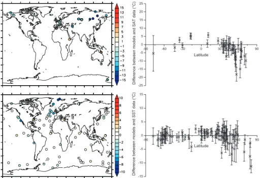
4.1 Point-based comparison of SATs and SSTs

Figure 5 shows a traditional comparison of point-based proxy temperature anomalies to the MMM anomalies derived from Experiment 2. This analysis assesses the de-gree of ade-greement between the temperature anomalies of proxies and models, rather

5

than comparing absolute temperature estimates. On land, terrestrial temperature es-timates are derived from Salzmann et al. (2008, 2012). In the Southern Hemisphere and tropics MMM SAT anomalies are within 3◦C of proxy anomalies. In the North-ern Hemisphere, particularly beyond 40◦N, the MMM underestimates the magnitude of SAT warming by as much as 15◦C. For the oceans, SST anomalies are derived

10

from Dowsett et al. (2010, 2012). The analysis shown in Fig. 5 demonstrates a broad concordance between data and models apart from in the Northern North Atlantic and Nordic Seas. Here the MMM underestimates the magnitude of change by as much as 8 to 10◦C. The calculated 2σon the MMM SAT and SST anomalies indicates that the majority of the discrepancies between model results and proxy estimates are not

statis-15

tically significant to a 95 % confidence interval. Nevertheless, data and models outputs for the Nordic Seas and Russia/Siberia remain significantly different.

4.2 Regional-scale comparison of SSTs and SATs

Due to the di_fferent spatial scales considered by proxy data and model outputs, it is perhaps unsurprising to observe the kind of discord between proxies and model

re-20

sults seen in Fig. 5. To test the validity of the comparison previously shown, and in an e_ffort to identify patterns of data/model discord which are regionally applicable, proxy and model simulations at a regional and seasonal scale were analysed (Fig. 6). The globe was subdivided into the seven continents in the terrestrial realm and the seven major ocean basins in the marine regime. Proxy temperature anomalies pertaining to

25

(16)

CPD

8, 2969–3013, 2012

Project

Title Page

Tables Figures

◭ ◮

Back Close

Full Screen / Esc

Discussion

P

a

per

|

Dis

cussion

P

a

per

|

Discussion

P

a

per

|

Discussio

n

P

a

per

analysis SST calculation methods provide information on cold and warm month SSTs (Dowsett et al., 2010, 2012). Available Mg/Ca and alkenone palaeothermometry-based estimates available for a sub-section of marine sites provide additional information on mean annual SSTs (Dowsett et al., 2010, 2012). These estimates are compared to regional mean annual and monthly changes in temperature computed from the

Ex-5

periment 2 (marine and terrestrial regions) and Experiment 1 (terrestrial regions only) multi-model means. The calculated 2σ for SAT and SST derived from the ensemble members is also included (Fig. 6).

In this analysis, the general agreement between model outputs and SST proxy es-timates for the Southern Ocean, North and South Pacific, Indian and South Atlantic

10

Oceans highlighted in Fig. 5 is reiterated. In the Arctic Ocean, the model/data discord persists but is only marked when the model results are compared to geochemically-based proxy mean annual SST estimates, rather than faunal analysis-geochemically-based estimates for cold and warm month means. Data/model discord in this region should be viewed cautiously unless multi-proxy temperature estimates become available from each

ma-15

rine locality in the Arctic.

For the North Atlantic, the regional comparison indicates concordance between the models and proxy data. This is in contrast to the analysis shown in Fig. 5 where the North Atlantic was shown as a region of major data/model discord. In some respects this is to be expected as as the analysis in Fig. 6 averages out the large meridional SST

20

gradient in the proxy data which is not fully reproduced by the models. However, this analysis may also indicate that models’ are capable of simulating the average amount of warming in the North Atlantic as a whole, whilst not necessarily reproducing the exact distribution of the SST increases vis-a-vis the PRISM3D localities used for SST reconstruction. Given the complex oceanography and steep SST gradients which exist

25

in the North Atlantic (e.g. Kelly et al., 2010), this outcome is not unexpected given the resolution of the ocean models used in this study.

(17)

CPD

8, 2969–3013, 2012

Project

Title Page

Tables Figures

◭ ◮

Back Close

Full Screen / Esc

Discussion

P

a

per

|

Dis

cussion

P

a

per

|

Discussion

P

a

per

|

Discussio

n

P

a

per

|

the degree of MAT increase compared to the proxy data. Differences over Australia are at the limits of detection, while the single point over Antarctica is not representative of continental scale warming and suffers from uncertain chronology (Hill et al., 2007). Over Asia the analyses shown in Figs. 5 and 6 highlight the greater degree of warming reconstructed in the continental interior and high-latitudes in the proxies compared to

5

the MMMs.

5 Calculation of Earth system sensitivity

5.1 What is Earth system sensitivity?

Climate Sensitivity (the temperature response of the Earth to elevated CO₂ concentra-tions) is a concept which has received much attention, as it is a simple and

easily-10

understood metric which gives a first-order indication of the magnitude of possible future climate change given increased CO₂ emissions (e.g. Charney, 1979; Hansen et al., 2008; Meinshausen et al., 2009).

Estimates of Climate Sensitivity which are based on models are normally defined as the modelled global mean near-surface air temperature equilibrium response to a

sus-15

tained doubling of atmospheric CO₂concentration. In general, model-based estimates of climate sensitivity are most relevant for short timescales (<100 yr), as typical cli-mate models do not include feedbacks which act on longer timescales, and/or are not often run out to full equilibrium (Lunt et al., 2010). Furthermore, no model includes all possible feedbacks even on short timescales (for example, feedbacks associated with

20

atmospheric chemistry and and aerosols are only just being included in state-of-the-art models).

Earth System Sensitivity (ESS) has been defined by Lunt et al. (2010) as the equi-librium global mean near-surface air temperature equiequi-librium response to a sustained doubling of atmospheric CO₂ concentrations, including all feedbacks and processes

25

(18)

CPD

8, 2969–3013, 2012

Project

Title Page

Tables Figures

◭ ◮

Back Close

Full Screen / Esc

Discussion

P

a

per

|

Dis

cussion

P

a

per

|

Discussion

P

a

per

|

Discussio

n

P

a

per

timescale feedbacks, models can be used to estimate ESS. Palaeo data are very use-ful tools in determining ESS, as they provide the potential for an independent test of ESS.

5.2 Previous estimates of ESS using the mPWP

The mPWP is useful for investigating the concept of ESS because it represents a world

5

in quasi-equilibrium with high CO2, for a sufficient period that long-term feedbacks are

close to equilibrium. Using a combined model-data approach, Lunt et al. (2010) esti-mated ESS to be between 30 % and 50 % greater than CS. They took a climate model (HadCM3), and imposed changes to the CO2, orography, ice sheet and vegetation

model boundary conditions which were consistent with changes observed in the palaeo

10

record. They then evaluated the model simulation relative to mPWP SST records. Fi-nally, they used a series of sensitivity studies to eliminate the orographic forcing effect, arguing that the remaining temperature signal was an approximation to ESS.

5.3 Using PlioMIP Experiment 2 to inform estimates of ESS

Here, we use the PlioMIP simulations from Experiment 2 to estimate ESS, using a

sim-15

ilar approach to Lunt et al. (2010). Since the PRISM3D orography in the PlioMIP ex-perimental design is similar to modern (Sohl et al., 2009), our approach is actually significantly simpler than Lunt et al. (2010) because we argue that in this case, the orographic effect is negligible. In the PRISM2 data set, which was used to provide the boundary consditions for the Lunt et al. (2010) estimates, mPWP and modern

oro-20

graphies were less similar. As such, we consider the elevated CO₂to be the ultimate forcing of the simulated mPWP warmth, and thus our simulations represent the equi-librium state of a world at 405 ppmv of CO2. To convert this to the usual definition of

ESS (i.e. a CO₂doubling from 280 to 560 ppmv), the Pliocene warming is multiplied by ln(560.0/280.0)/ln(405.0/280.0)₌1.88. The global mean values are given in Table 2

25

(19)

CPD

8, 2969–3013, 2012

Project

Title Page

Tables Figures

◭ ◮

Back Close

Full Screen / Esc

Discussion

P

a

per

|

Dis

cussion

P

a

per

|

Discussion

P

a

per

|

Discussio

n

P

a

per

|

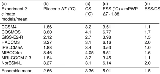
and the ratio ESS/CS. There is a large spread in the ratio ESS/CS from 1.04 (the IPSL model) to 1.99 (HadCM3). The ratio for the ensemble mean is 1.5. Therefore, the PlioMIP simulations give us high confidence that ESS>CS, and moderate confidence that ESS/CS is between 1 and 2.

One caveat to this calculation of ESS is that changes in the Earth’s orbit are not

5

relevant to calculations of either CS or ESS. If reconstructed changes in global ice vol-ume or vegetation distribution (i.e. longer term feedbacks) are even partly a function of orbital variability rather than CO2, the utility of the current experiments for

under-standing the sensitivity of climate in the context of future climate change is diminished. Initial transient mid-Pliocene climate simulations using Earth System Model of

Interme-10

diate Complexity are becoming available (Ganopolski et al., 2011). Here CO₂ forcing and orbital forcing have been imposed in isolation and in concert, and have suggested that a significant percentage of the additional feedback to global temperature derived from changes in vegetation cover and ice sheet extent are attributable to orbital forcing (Ganopolski et al., 2011).

15

6 Discussion and future outlook

6.1 PlioMIP phase 2: recognising and reducing uncertainties (the PMIP Triangle)

The marine point-based DMC shown in Fig. 5 demonstrates that even in the region where the proxy-derived SST anomalies are at their greatest, the 2σ calculated from

20

the PlioMIP ensemble makes it difficult to attribute statistical significance to the vast majority of site by site data/model mismatches at a 95 % confidence level. This result does not consider the variability and uncertainty of the proxy-estimated SST anoma-lies (see Dowsett et al. 2012). Therefore, whilst the extent of data/model mismatch may appear substantial, when the above points are considered, no discord between

25

(20)

CPD

8, 2969–3013, 2012

Project

Title Page

Tables Figures

◭ ◮

Back Close

Full Screen / Esc

Discussion

P

a

per

|

Dis

cussion

P

a

per

|

Discussion

P

a

per

|

Discussio

n

P

a

per

difficult for proxy-data or climate modelling to meaningfully inform the other regarding performance, until uncertainties in the reconstruction as well as modelling of Pliocene warmth are better quantified and then reduced.

In any palaeo data/model comparison the cause of data/model mismatches will be complex and not attributable to a single factor in either the models or proxy data. In the

5

context of PMIP three high level causes of data/model discord require consideration. The first is limitations in the underlying numerical representation of processes in mod-els, the second is uncertainties in the interpretation of proxy records, and the third is limitations of experimental design within models. This triangle of uncertainty, which we term the PMIP Triangle, serves as a useful guide to establish a well-balanced

assess-10

ment of the causes of disagreement between proxy data and model outputs.

In terms of the climate modelling for the Pliocene, PlioMIP is an effective means to quantify uncertainties in model predictions (the modelling vertex of the PMIP Trian-gle). So far PlioMIP has identified an envelope of climate possible from a collection of atmosphere-only and coupled atmosphere-ocean climate models set up to produce

15

a single realisation of climate for the mPWP. Given the known unknowns in providing models with “correct” boundary conditions for the mPWP, it would be advantageous for PlioMIP Phase 2 to focus on identifying a number of key sensitivity experiments to examine how poor constraints on atmospheric trace gasses, ice sheet configura-tions, palaeogeography and bathymetry could ameliorate the magnitude of data/model

20

discord seen in the high-latitudes of the Northern Hemisphere. Outlining a series of potential sensitivity tests, and allowing modelling groups to select which experiment or experiments they wish to run, would facilitate an efficient exploration of boundary condition uncertainty (experimental design vertex of the PMIP Triangle).

The final vertex of the PMIP Triangle to be considered is uncertainties in the

inter-25

(21)

CPD

8, 2969–3013, 2012

Project

Title Page

Tables Figures

◭ ◮

Back Close

Full Screen / Esc

Discussion

P

a

per

|

Dis

cussion

P

a

per

|

Discussion

P

a

per

|

Discussio

n

P

a

per

|

the Pliocene to which the ages of marine or terrestrial sites could be more confidently attributed (Dowsett and Poore, 1991). It also naturally increased the potential amount of geological data that could be incorporated, and would therefore underpin any en-vironmental reconstruction. The current PRISM time slab for marine reconstruction is 240 000 yr wide. The vegetation reconstruction is constructed by considering

informa-5

tion from the entire Piacenzian Stage (1 million yr wide).

So what exactly does the PRISM environmental reconstruction represent? At each individual site it is an average of warm climate signals that occurred during the time slab (Dowsett et al., 2010; Salzmann et al., 2008). It should not be considered as a re-construction of environmental conditions that could have existed together at a discrete

10

moment in time (i.e. a time slice). In terms of mPWP climate modelling studies using AGCMs this does not present a problem. The PRISM3D reconstruction allows AGCMs to examine what a global average warm climate during the mid-Pliocene might have looked like (e.g. Chandler et al., 1994; Sloan et al., 1996; Haywood et al., 2000).

However, outputs from the AOGCMs shown here have highlighted disconnections

15

between the proxy data, which is representative of a time slab, and relatively short model integrations that predict an equilibrium climate state based on constant external forcing (see also Dowsett et al., 2012; Haywood et al., 2012). So whilst there have been a number of attempts to evaluate AOGCMs against the PRISM data set, including the DMC shown here, it is important to appreciate that neither the proxy data nor the

20

climate models (due to the prescribed boundary conditions) are actually reproducing the same objective, a discrete moment in time during the mPWP.

In reality, climate model simulations run for 500 integrated years, using only a single realisation of orbit, CO2and other forcings, cannot reproduce a reconstruction of

aver-age warm climate conditions (over either 240 000 or 1 million yr), which reflect multiple

25

(22)

CPD

8, 2969–3013, 2012

Project

Title Page

Tables Figures

◭ ◮

Back Close

Full Screen / Esc

Discussion

P

a

per

|

Dis

cussion

P

a

per

|

Discussion

P

a

per

|

Discussio

n

P

a

per

future relies upon the identification of a discrete time slice, or slices, for environmental reconstruction within the Pliocene epoch.

6.2 PlioMIP: towards the identification and adoption of a Pliocene time slice(s)

Any criteria established to aid in the identification of a Pliocene time slice(s) for palaeoenvironmental reconstruction will be subjective. In essence the criteria will be

5

dependent upon specific scientific circumstances and the aim and objectives of the study. Given the potential utility of the Pliocene to understand the dynamics of warm climates, as well as elucidate Climate/Earth System Sensitivity, Haywood et al. (2012) proposed that a time slice displaying a near modern orbital configuration within a known warm peak in the benthic oxygen isotope record would represent the most logical

10

choice for an initial time slice reconstruction. Such a strategy also has the advantage of simplifying the interpretation of geological proxies, because palaeo-seasonality has more chance of being the same or very similar to modern seasonality.

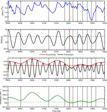
The Haywood et al. (2012) recommendation for an initial time slice at 3.205 Ma BP for reconstruction sits in the normal polarity of the Gauss Chron between the Kaena

15

(above) and Mammoth (below) reversals (Fig. 7). The peak deviation in benthicδ18O is centred on Marine Isotope Stage KM5c (or KM5.3). The 0.21 to 0.23‰ deviation in

δ18O could reflect a 21 to 23 m sea-level rise above modern (assuming 0.1‰ equates to∼10 m of sea level rise, Miller et al., 2012), providing that the signal is purely a

func-tion of ice volume rather than any change in deep ocean temperatures. Assuming the

20

near-total loss of the West Antarctic and Greenland ice sheets (a reasonable initial premise given proxy data and model outputs; Naish et al., 2009; Pollard and DeConto, 2009; Dolan et al., 2011; Lunt et al., 2008), volume reduction from the East Antarctic ice sheet is a moderate 6 or 7 m of ice volume equivalent. This general interpreta-tion of sea-level from the LR04 stack is supported by a recent synthesis of sea-level

25

records between 2.9 and 3.3 Ma BP by Miller et al. (2012). At∼3.205 Ma BP the Miller

et al. (2012) synthesis indicates a maximum sea-level rise of 25 m±10 m (derived from

(23)

CPD

8, 2969–3013, 2012

Project

Title Page

Tables Figures

◭ ◮

Back Close

Full Screen / Esc

Discussion

P

a

per

|

Dis

cussion

P

a

per

|

Discussion

P

a

per

|

Discussio

n

P

a

per

|

sea-level records for approximately the same time indicates a peak sea-level rise of

∼22 m±10 m.

During the time-slice, orbital forcing is close to the modern distribution both sea-sonally and regionally (Haywood et al., 2012). Available proxy data for atmospheric CO₂ (e.g. Bartoli et al., 2011) places an upper limit of ∼400 ppmv, with a cluster of

5

four measurements within 100 ka using three different proxy techniques (alkenones, boron isotopes and stomatal density) indicating a range of between 300 to 380 ppmv (Haywood et al., 2012).

7 Conclusions

We present, for the first time, a systematic model intercomparison and model-data

10

comparison of the results from eleven climates models simulating the mid-Pliocene Warm Period. This study includes outputs from atmosphere-only (Experiment 1; includ-ing outputs from seven models) as well as coupled atmosphere-ocean climate models (Experiment 2; including outputs from eight models). Model results show a range of global mean surface temperature anomalies, even though the models were specified

15

with identical boundary conditions. In other words, models interpret the amount of forc-ing derived from Pliocene boundary conditions di_fferently. For Experiment 2, the range in global annual mean surface air temperature warming is 1.76◦C. For sea surface and surface air temperature, the models are least consistent in the North Atlantic and in the high-latitudes. For precipitation they are least consistent in the tropics. Whilst all

mod-20

els predict an enhancement of the hydrological cycle, the magnitude of this enhance-ment is variable, and regional disparities in total precipitation are apparent. All models simulate a polar amplification of surface air temperature warming for the Pliocene, al-though the magnitude of this amplification is model dependant. Our ensembles support previous work suggesting that Earth System Sensitivity (ESS) is greater than Climate

25

(24)

CPD

8, 2969–3013, 2012

Project

Title Page

Tables Figures

◭ ◮

Back Close

Full Screen / Esc

Discussion

P

a

per

|

Dis

cussion

P

a

per

|

Discussion

P

a

per

|

Discussio

n

P

a

per

Within the ensemble range, the models appear able to reproduce many of the sea-surface and sea-surface air temperature anomalies reconstructed from multiple proxies in the Southern Hemisphere, the tropics, and in the Northern Hemisphere (to∼40◦N). At

higher latitudes in the Northern Hemisphere point-to point data/model comparisons in-dicate that models underestimate the magnitude of change on land and in the oceans.

5

Comparisons of regional averages highlight that Russia and Siberia as particular areas of concern. However, much of the signal of data/model discord in the Northern Hemi-sphere is not significant at a 95 % confidence interval, and this conclusion is drawn before uncertainties in geological proxies are included. Whilst these results provide jus-tification for new sensitivity studies specifically targeted towards improving the match

10

between data and models in the higher-latitudes of the Northern Hemisphere, they also highlight the need for reduced uncertainties in temperature estimates from geo-logical temperature proxies. We outline a strategy towards the adoption of more tightly constrained time slices, rather than the current time slab approach (where proxy data may be derived from a window of time as wide as one million years), to help reduce

15

uncertainties in proxy data and the experimental design used in future climate model simulations. Such a combined approach will allow for assessments of model perfor-mance for the Pliocene to be made with greater confidence in the future.

Supplementary material related to this article is available online at:

http://www.clim-past-discuss.net/8/2969/2012/cpd-8-2969-2012-supplement.

20

pdf.

Acknowledgements. A. M. H., A. M. D and S. J. P acknowledge that the research leading to these results has received funding from the European Research Council under the European Union’s Seventh Framework Programme (FP7/2007-2013)/ERC grant agreement no. 278636. A. M. D acknowledges the UK Natural Environment Research Council for the provision of a

Doc-25

(25)

CPD

8, 2969–3013, 2012

Project

Title Page

Tables Figures

◭ ◮

Back Close

Full Screen / Esc

Discussion

P

a

per

|

Dis

cussion

P

a

per

|

Discussion

P

a

per

|

Discussio

n

P

a

per

|

Survey for financial support. C. S. and G. L. received funding through POLMAR and PACES. Z. Z. would like to thank Mats Bentsen, Jerry Tjiputra, Ingo Bethke from Bjerknes Center for Cli-mate Research for the contribution to the development of the NorESM-L. D. J. L acknowledges Research Councils UK for the award of an RCUK fellowship and the Leverhulme Trust for the award of a Phillip Leverhulme Prize. B. L. O and N. A. R recognise that NCAR is sponsored

5

by the US National Science Foundation (NSF) and computing resources were provided by the Climate Simulation Laboratory at NCAR’s Computational and Information Systems Laboratory (CISL), sponsored by the NSF and other agencies. The source code of MRI model is provided by S. Yukimoto, O. Arakawa, and A. Kitoh in Meteorological Research Institute, Japan. Funding for L. S. and M. C. provided by NSF Grant ATM0323516 and NASA Grant NNX10AU63A.

W.-10

L.C and A.A-O. would like to thank R. Ohgaito for help in setting up the MIROC4m experiments which were run on the Earth Simulator at JAMSTEC.

References

Bartoli, G., H ¨onisch, B., and Zeebe, R. E.: Atmospheric CO₂ decline during the Pliocene intensification of Northern Hemisphere glaciations, Paleoceanography, 26, PA4213,

15

doi:10.1029/2010PA002055, 2011.

Bonan, G. B., Oleson, K. W., Vertenstein, M., Levis, S., Zeng, X., Dai, Y., Dickinson, R. E., and Yang, Z.-L.: The land surface climatology of the Community Land Model coupled to the NCAR Community Climate Model, J. Climate, 15, 3123–3149, 2002.

Braconnot, P., Otto-Bliesner, B., Harrison, S., Joussaume, S., Peterchmitt, J.-Y., Abe-Ouchi, A.,

20

Crucifix, M., Driesschaert, E., Fichefet, Th., Hewitt, C. D., Kageyama, M., Kitoh, A., La ˆan ´e, A., Loutre, M.-F., Marti, O., Merkel, U., Ramstein, G., Valdes, P., Weber, S. L., Yu, Y., and Zhao, Y.: Results of PMIP2 coupled simulations of the Mid-Holocene and Last Glacial Maxi-mum – Part 1: experiments and large-scale features, Clim. Past, 3, 261–277, doi:10.5194/cp-3-261-2007, 2007.

25

(26)

CPD

8, 2969–3013, 2012

Project

Title Page

Tables Figures

◭ ◮

Back Close

Full Screen / Esc

Discussion

P

a

per

|

Dis

cussion

P

a

per

|

Discussion

P

a

per

|

Discussio

n

P

a

per

Bragg, F. J., Lunt, D. J., and Haywood, A. M.: Mid-Pliocene climate modelled using the UK Hadley Centre Model: PlioMIP Experiments 1 and 2, Geosci. Model Dev. Discuss., 5, 837– 871, doi:10.5194/gmdd-5-837-2012, 2012.

Cattle, H. and Crossley, J.: Modelling arctic climate change, Philos. T. R. Soc. A, 352, 201–213, 1995.

5

Chan, W.-L., Abe-Ouchi, A., and Ohgaito, R.: Simulating the mid-Pliocene climate with the MIROC general circulation model: experimental design and initial results, Geosci. Model Dev., 4, 1035–1049, doi:10.5194/gmd-4-1035-2011, 2011.

Chandler, M., Rind, D., and Thompson, R.: Joint investigations of the middle Pliocene climate II: GISS GCM Northern Hemisphere results, Global Planet. Change, 9, 197–219, 1994.

10

Charney, J. G.: Carbon Dioxide and Climate: A Scientific Assessment, National Academy of Science, Washington, DC, 22 pp., 1979.

Collins, W. D., Rasch, P. J., Boville, B. A., Hack, J. J., McCaa, J. R., Williamson, D. L., Kiehl, J. T., and Briegleb, B.: Description of the NCAR Community Atmosphere Model (CAM3.0), NCAR Tech. Note NCAR/TN-464+STR, National Center for Atmospheric Research, Boulder, CO,

15

226 pp., 2004.

Contoux, C., Ramstein, G., and Jost, A.: Modelling the mid-Pliocene Warm Period climate with the IPSL coupled model and its atmospheric component LMDZ5A, Geosci. Model Dev., 5, 903–917, doi:10.5194/gmd-5-903-2012, 2012.

Cox, P. M., Betts, R. A., Bunton, C. B., Essery, R. L. H., Rowntree, P. R., and Smith, J.: The

20

impact of new land surface physics on the GCM simulation of climate and climate sensitivity, Clim. Dynam., 15, 183–203, 1999.

Cronin, T. M., Whatley, R. C., Wood, A., Tsukagoshi, A., Ikeya, N., Brouwers, E. M., and Briggs, W. M.: Microfaunal evidence for elevated mid-Pliocene temperatures in the Arctic Ocean, Paleoceanography, 8, 161–173, 1993.

25

Danabasoglu, G., Bates, S., Briegleb, B. P., Jayne, S. R., Jochum, M., Large, W. G., Pea-cock, S., and Yeager, S. G.: CCSM4 ocean component, J. Climate, 25, 1361–1389, 2012. Dufresne, J. L., Foujols, M. A., Denvil, S., Caubel, A., Marti, O., Aumont, O., Balkanski, Y.,

Bekki, S., Bellenger, H., Benshila, R., Bony, S., Bopp, L., Braconnot, P., Brockmann, P., Cad-ule, P., Cheruy, F., Codron, F., Cozic, A., Cugnet, D., de Noblet, N., Duval, J. P., Ethe, C.,

30

(27)

CPD

8, 2969–3013, 2012

Project

Title Page

Tables Figures

◭ ◮

Back Close

Full Screen / Esc

Discussion

P

a

per

|

Dis

cussion

P

a

per

|

Discussion

P

a

per

|

Discussio

n

P

a

per

|

J., Lott, F., Madecm, G., Mancip, M., Marchand, M., Masson, S., Meurdesoif, Y., Mignot, J., Musat, I., Parouty, S., Polcher, J., Rio, C., Schulz, M., Swingedouw, D., Szopa, S., Talandier, C., Terray, P., and Viovy, N.: Climate change projections using the IPSL-CM5 Earth System Model: from CMIP3 to CMIP5, Clim. Dynam., submitted, 2012.

Dekens, P. S., Ravelo, A. C., and McCarthy, M. D.: Warm upwelling regions in the Pliocene

5

Warm Period, Paleoceanography, 22, PA3211, doi:10.1029/2006PA001394, 2007.

Dolan, A. M., Haywood, A. M., Hill, D. J., Dowsett, H. J., Hunter, S. J., Lunt, D. J., and Pick-ering, S.: Sensitivity of Pliocene ice sheets to orbital forcing, Palaeogeogr. Palaeocl., 309, 98–110, 2011.

Dowsett, H. J. and Cronin, T. M.: High eustatic sea level during the Middle Pliocene: evidence

10

from the Southeastern US Atlantic Coastal Plain, Geology, 18, 435–438, 1990.

Dowsett, H. J. and Poore, R. Z.: Pliocene sea surface temperatures of the North Atlantic Ocean at 3.0 Ma, Quaternary Sci. Rev., 10, 189–204, 1991.

Dowsett, H. J., Robinson, M. M., and Foley, K. M.: Pliocene three-dimensional global ocean temperature reconstruction, Clim. Past, 5, 769–783, doi:10.5194/cp-5-769-2009, 2009.

15

Dowsett, H. J., Robinson, M., Haywood, A. M., Salzmann, U., Hill, D. J., Sohl, L., Chan-dler, M. A., Williams, M. Foley, K., and Stoll, D.: The PRISM3D paleoenvironmental recon-struction, Stratigraphy, 7, 123–139, 2010.

Dowsett, H. J., Haywood, A. M., Valdes, P. J., Robinson, M. M., Lunt, D. J., Hill, D. J., Stoll, D. K., and Foley, K. M.: Sea surface temperatures of the mid-Piacenzian Warm Period: a

compari-20

son of PRISM3 and HadCM3, Palaeogeogr. Palaeocl., 309, 83–91, 2011.

Dowsett, H. J., Robinson, M. M., Haywood, A. M., Hill, D. J., Dolan, A. M., Stoll, D. K., Chan, W. L., Abe-Ouchi, A., Chandler, M. A., Rosenbloom, N. A., Otto-Bleisner, B. L., Bragg, F. J., Lunt, D. J., Foley, K. M., and Riesselman, C. R.: Assessing confidence in Pliocene sea surface temperatures to evaluate predictive models, Nature Climate Change,

25

2, 365–371, doi:10.1038/NCLIMATE1455, 2012.

Dwyer, G. S. and Chandler, M. A.: Mid-Pliocene sea level and continental ice volume based on coupled benthic Mg/Ca palaeotemperatures and oxygen isotopes, Philos. T. R. Soc. A, 367, 157–168, 2009.

Fichefet, T. and Morales-Maqueda, M. A.: Sensitivity of a global sea ice model to the

30