www.biogeosciences.net/12/567/2015/ doi:10.5194/bg-12-567-2015
© Author(s) 2015. CC Attribution 3.0 License.
Secondary calcification and dissolution respond differently to future
ocean conditions
N. J. Silbiger and M. J. Donahue
University of Hawaii, at Manoa, Hawaii Institute of Marine Biology, PO Box 1346, Kaneohe, Hawaii
Correspondence to:N. J. Silbiger ([email protected])
Received: 8 August 2014 – Published in Biogeosciences Discuss.: 2 September 2014 Revised: 15 December 2014 – Accepted: 18 December 2014 – Published: 29 January 2015
Abstract. Climate change threatens both the accretion and erosion processes that sustain coral reefs. Secondary cal-cification, bioerosion, and reef dissolution are integral to the structural complexity and long-term persistence of coral reefs, yet these processes have received less research atten-tion than reef accreatten-tion by corals. In this study, we use cli-mate scenarios from RCP 8.5 to examine the combined ef-fects of rising ocean acidity and sea surface temperature (SST) on both secondary calcification and dissolution rates of a natural coral rubble community using a flow-through aquarium system. We found that secondary reef calcification and dissolution responded differently to the combined effect ofpCO2and temperature. Calcification had a non-linear
re-sponse to the combined effect of pCO2 and temperature:
the highest calcification rate occurred slightly above ambi-ent conditions and the lowest calcification rate was in the highest temperature–pCO2 condition. In contrast,
dissolu-tion increased linearly with temperature–pCO2. The rubble
community switched from net calcification to net dissolution at+271 µatmpCO2and 0.75◦C above ambient conditions,
suggesting that rubble reefs may shift from net calcification to net dissolution before the end of the century. Our results indicate that (i) dissolution may be more sensitive to climate change than calcification and (ii) that calcification and dis-solution have different functional responses to climate stres-sors; this highlights the need to study the effects of climate stressors on both calcification and dissolution to predict fu-ture changes in coral reefs.
1 Introduction
In 2013, atmospheric carbon dioxide (CO2(atm)) reached an unprecedented milestone of 400 ppm (Tans and Keel-ing, 2013), and this rising CO2(atm)is increasing sea surface temperature (SST) and ocean acidity (Caldeira and Wickett, 2003; Cubasch et al., 2013; Feely et al., 2004). Global SST has increased by 0.78◦C since pre-industrial times (Cubasch et al., 2013), and it is predicted to increase by another 0.8– 5.7◦C by the end of this century (Meinshausen et al., 2011; Van Vuuren et al., 2008; Rogelj et al., 2012). The Hawaii Ocean Time-series detected a 0.075 decrease in mean annual pH at station ALOHA over the past 20 years (Doney et al., 2009) and there have been similar trends at stations around the world, including the Bermuda Atlantic Time-series and the European Station for Time-series Observations in the ocean (Bindoff et al., 2007). pH is expected to drop by an additional 0.14–0.35 pH units by the end of the twenty-first century (Bopp et al., 2013). All marine ecosystems are at risk from rising SST and decreasing pH (Doney et al., 2009; Hoegh-Guldberg et al., 2007; Hoegh-Guldberg and Bruno, 2010), but coral reefs are particularly vulnerable to these stressors (reviewed in Hoegh-Guldberg et al., 2007).
by non-coral invertebrates and calcareous algae), bioerosion, and reef dissolution that are integral to maintaining the struc-tural complexity and net growth of coral reefs has received less attention (Andersson and Gledhill, 2013; Andersson et al., 2011; Andersson and Mackenzie, 2012). Bioerosion and dissolution break down the reef framework, while secondary calcification helps maintain reef stability by cementing the reef together (Adey, 1998; Camoin and Montaggioni, 1994; Littler, 1973) and producing chemical cues that induce settle-ment of many invertebrate larvae including several species of corals (Harrington et al., 2004; Price, 2010). Coral reefs will only persist if constructive reef processes (growth by corals and secondary calcifiers) exceed destructive reef processes (bioerosion and dissolution). In this study, we examine the combined effects of rising ocean acidity and SST on both calcification and dissolution rates of a natural community of secondary calcifiers and bioeroders.
Recent laboratory experiments have focused on the re-sponse of individual taxa of bioeroders or secondary calci-fiers to climate stressors. For example, studies have specif-ically addressed the effects of rising ocean acidity and/or temperature on bioerosion by a clionid sponge (Wisshak et al., 2012, 2013; Fang et al., 2013) and a community of pho-tosynthesizing microborers (Tribollet et al., 2009; Reyes-Nivia et al., 2013). These studies found that bioerosion in-creased under future climate change scenarios. Several stud-ies have focused on tropical calcifying algae and have found decreased calcification (Semesi et al., 2009; Johnson et al., 2014; Comeau et al., 2013; Jokiel et al., 2008; Kleypas and Langdon, 2006) and increased dissolution (Diaz-Pulido et al., 2012) with increasing ocean acidity and/or SST. How-ever, the bioeroding community is extremely diverse, and can interact with the surrounding community of secondary calcifiers: for example, crustose coralline algae (CCA) can inhibit internal bioerosion (White, 1980; Tribollet and Payri, 2001). To understand the combined response of bioeroders and secondary calcifiers, we take a community perspective and examine the synergistic effects of rising SST and ocean acidity on a natural community of secondary calcifiers and bioeroders. Using the total alkalinity anomaly technique, we test for net changes in calcification during the day and dis-solution (most of which is caused by bioeroders; Andersson and Gledhill, 2013) at night. Our climate change treatments are modeled after the Representative Concentration Pathway (RCP) 8.5 climate scenario (Van Vuuren et al., 2011; Mein-shausen et al., 2011), one of the high-emission scenarios used in the most recent Intergovernmental Panel on Climate Change (IPCC) report (Cubasch et al., 2013). The RCP 8.5 scenario predicts an increase in temperature of 3.8–5.7◦C (Rogelj et al., 2012) and an increase in atmospheric CO2of
557 ppm by the year 2100 (Meinshausen et al., 2011). We use the RCP 8.5 scenario because the current CO2concentrations
are tracking just above what this scenario predicts (Sanford et al., 2014). While prior studies have focused on the contribu-tions of individual community members to increased
temper-ature and CO2, here, we examine the community response to
the RCP 8.5 climate scenario and measure calcification, dis-solution, and net community production rates.
2 Materials and methods 2.1 Collection site
All collections were made on the windward side of Moku o Lo‘e (Coconut Island) in Kaneohe Bay, Hawaii adjacent to the Hawaii Institute of Marine Biology. This fringing reef is dominated byPorites compressaandMontipora capitata,
with occasional colonies ofPocillopora damicornis,Fungia scutaria, andPorites lobata. Kaneohe Bay is a protected,
semi-enclosed embayment; the residence time can be more than 1 month long in the protected southern portion of the bay (Lowe et al., 2009a, 2009b) that is coupled with a high daily variance in pH (Guadayol et al., 2014). The wave action is minimal (Smith et al., 1981; Lowe et al., 2009a; Lowe et al., 2009b), and currents are relatively slow (5 cm s−1 maxi-mum) and wind driven (Lowe et al., 2009a, 2009b).
2.2 Sample collection
We collected pieces of deadPorites compressacoral
skele-ton (hereafter, referred to as rubble) as representative com-munities of bioeroders and secondary calcifiers. Rubble was collected with a hammer and chisel from a shallow reef flat (∼1 m depth) in November 2012. Only pieces of rubble without any live coral were collected. The rubble commu-nity in Kaneohe Bay is comprised of secondary calcifiers, in-cluding CCA from the generaHydrolithon,Sporolithon, and Peyssonnelia, and non-coral calcifying invertebrates (e.g.,
boring bivalves (Lithophaga fasciola and Barbatia divari-cate), oysters (Crassostrea gigas), and small crustaceans),
filamentous and turf algae, and internal bioeroders, including boring bivalves (L. fasciolaandB. divaricate), sipunculids
(Aspidosiphon elegans,Lithacrosiphon cristatus, Phascolo-soma perlucens, andPhascolosoma stephensoni), phoronids
(Phoronis ovalis), sponges (Clionaspp.) and a diverse
as-semblage of polychaetes (White, 1980). All rubble pieces were combined after collection and maintained in a 100 L flow-through tank with ambient seawater from Kaneohe Bay until random assignment to treatments.
2.3 Experimental design
The Hawaii Institute of Marine Biology (HIMB) hosts a mesocosm facility with flow-through seawater from Kaneohe Bay and controls for light, temperature,pCO2, and flow rate.
The facility is comprised of 24 experimental aquaria split be-tween four racks; each rack has a 150 L header tank that feeds six experimental aquaria, each 50 L in volume (Fig. 1).
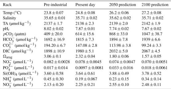
Table 1.Means and standard errors of all measured parameters by rack.pCO2, HCO−3 ,CO23−, DIC, andaragwere all calculated from
the measured TA and pH samples using CO2SYS. Each table entry is the mean of 12 water samples: one daytime sample and one nighttime sample for six aquaria within a rack. Data are all from the imposed treatment conditions with no rubble inside the aquaria.
Rack Pre-industrial Present day 2050 prediction 2100 prediction
Temp (◦C) 23.8±0.07 24.8±0.08 26.2±0.06 27.2±0.08 Salinity 35.65±0.01 35.71±0.02 35.62±0.02 35.71±0.02
TA (µmol kg−1) 2137±1.7 2138±2.3 2139±2.0 2142±1.9
pHt 8.02±0.02 7.87±0.01 7.74±0.02 7.67±0.02
pCO2(µatm) 409±20.0 614±15.6 868±33.0 1047±38.7
HCO−
3 (µmol kg−1) 1692±16.9 1815±7.3 1894±7.8 1939±6.6
CO2−
3 (µmol kg−1) 194.20±6.7 147.08±2.8 113.98±3.8 99.24±3.3
DIC (µmol kg−1) 1898±10.9 1980±5.1 2032±5.0 2067±4.5
arag 3.06±0.1 2.32±0.04 1.80±0.06 1.57±0.05
NO−
2 (µmol L−1) 0.082±0.0028 0.078±0.0045 0.074±0.0047 0.070±0.0051
PO3−
4 (µmol L−1) 0.017±0.014 0.0097±0.0081 0.033±0.016 0.018±0.0061
Si(OH)4(µmol L−1) 3.60±0.58 3.64±0.61 3.88±0.49 3.78±0.52
NH+
4 (µmol L−1) 0.45±0.30 0.19±0.067 0.23±0.15 0.34±0.14
NO−
3 (µmol L−1) 2.13±0.20 2.25±0.21 2.55±0.10 2.48±0.11
}
}
}
Filtered Ambient Seawater
Header Tanks
Individual Aquaria Flow
Temperature
Rack Light
pCO2
Figure 1.A schematic of the mesocosm system at the Hawaii Insti-tute of Marine Biology. Ambient seawater is pumped into the sys-tem from a nearby fringing reef in Kaneohe Bay. The seawater is filtered with a sand trap filter, passed through a water chiller and then fed into one of four header tanks. pCO2 is manipulated in
each header tank by bubbling a mixture of CO2-free air and pure
CO2to the desired concentration. The water from one header tank flows into six aquaria (a rack). Light is controlled by a rack with metal-halide lights. There are two metal-halide lights per rack, with each light oscillating over a set of three aquaria. Flow and tempera-ture are controlled in each individual aquarium with flow valves and aquarium heaters and coolers, respectively.
temperature, and salinity from all aquaria to demonstrate the consistency of water conditions across aquaria without any rubble present (Table 1). The long-term temporal stability of the mesocosm system is reported in Putnam (2012). We then conducted “control” and “treatment” experiments to de-termine how RCP 8.5 predictions affect daytime calcifica-tion and nighttime dissolucalcifica-tion rates in a natural rubble com-munity. The first “control experiment” characterized base-line calcification and dissolution in each aquarium caused
by differences in rubble communities. In the second “treat-ment experi“treat-ment”, we manipulatedpCO2 and temperature
to simulate four climate scenarios (pre-industrial, present day, 2050, and 2100) and tested the response of calcifica-tion, dissolucalcifica-tion, and net community production. Each exper-iment used the TA anomaly method (Smith and Key, 1975; Andersson et al., 2009). This method calculates net calcifi-cation from changes in TA, and calculates net community production from changes in total dissolved inorganic carbon (DIC) adjusted for changes in carbon due to calcificaiton. Be-cause estimates of calcification are based on changes in TA, this method does not account for mechanical erosion (e.g., small chips of CaCO3 produced by sponge erosion).
How-ever, given the short duration of the experiment and the types of bioeroders present, we expect that chemical dissolution captured a significant proportion of the erosion in the sys-tem.
Approximately 1.2 L of rubble (3–4 pieces of weight 499±148 g and skeletal density 1.53±0.1 g cm−3 (mean ±SD,n=85)) were placed in each of the 24 experimental aquaria and acclimated to tank conditions in ambient sea-water for 3 days. On the fourth day, we performed the con-trol experiment, calculating daytime calcification and night-time dissolution for rubble in ambient seawater conditions using the TA anomaly technique. The next day we manipu-lated seawaterpCO2 and temperature to replicate four
cli-mate scenarios for the treatment experiment: pre-industrial (−1±0.057◦C and −205±11.9 µatm), present day (natu-ral Kaneohe Bay seawater 24.8±0.09◦C, 614±15.6 µatm), 2050 (+1.4±0.09◦C and +255±31 µatm), and 2100 (+2.4±0.08 and+433±40 µatm). Note that all changes in temperature and pCO2 were made relative to present-day
is consistently high relative to the open ocean and can range from 196 to 976 µatm in southern Kaneohe Bay, depending on conditions (Drupp et al., 2013). The yearly averagepCO2
at our collection site ranged from 565 to 675 µatm (Silbiger et al., 2014). After an acclimation time of 7 days, we sampled the treatment experiment, calculating daytime calcification and nighttime dissolution over a 24 h period.
During both experiments, TA, pH, salinity, temperature, and dissolved inorganic nutrient (DIN) samples were col-lected every 12 h over a 24 h period: just before lights-on in the morning (time 1) and just before lights-off at night (time 2) to capture light conditions, and then again before lights-on the next morning (time 3) to capture dark condi-tions. Flow into each aquarium was monitored and adjusted every 3 hours to ensure a consistent flow rate over the 24 h experiment. We calculated net ecosystem calcification and net community production using a simple box model (An-dersson et al., 2009) and normalized all our calculations to the surface area of the rubble in each tank. The surface area of the rubble was calculated using the wax dipping technique (Stimson and Kinzie III, 1991) at the end of the experiment.
2.4 Mesocosm setup
The mesocosm facility (Fig. 1) is supplied with ambient sea-water from Kaneohe Bay, which is filtered through a sand filter, passed through a water chiller (Aqualogic Multi Temp MT-1 model no. 2TTB3024A1000AA), and then fed into one of the four header tanks.pCO2was manipulated using a CO2
gas blending system (see Fangue et al., 2010; Johnson and Carpenter, 2012). Each targetpCO2concentration was
cre-ated by mixing CO2-free atmospheric air with pure CO2
us-ing mass flow controllers (C100L Sierra Instruments). Out-putpCO2was analyzed using a calibrated infrared CO2
an-alyzer (A151, Qubit Systems). CO2mixtures were then
bub-bled into one of the four header tanks and water from each individual header tank fed into the six individual treatment aquaria (Fig. 1). ThepCO2in each treatment aquarium was
estimated with CO2SYS (Van Heuven et al., 2011) using pH
and TA as the parameters.
Temperature was manipulated in each treatment aquar-ium using dual-stage temperature controllers (Aqualogic TR115DN). The temperature was continuously monitored with temperature loggers (TidbiT v2 Water Temperature Data Logger, sampling every 20 min), and point measure-ments were taken during every sampling period with a hand-held digital thermometer (Traceable Digital Thermome-ter, Thermo Fisher Scientific; precision=0.001◦C). Light was controlled by positioning an oscillating pendant metal-halide light (250 W) over a set of three aquaria and was programmed to emit an equal amount of light to each tank (∼500 µE of light). Lights were set to a 12 h : 12 h light to dark photoperiod and were monitored using a LI-COR spherical quantum PAR sensor. Flow rate was main-tained at 115±1 mL min−1, resulting in a residence time of
7.3±0.07 h per tank. Each aquarium was equipped with a submersible powerhead pump (Sedra KSP-7000 powerhead) to ensure that the tank was well mixed.
2.5 Seawater chemistry
All sample collection and storage vials were cleaned in a 10 % HCl bath for 24 h and rinsed three times with MilliQ water before use and rinsed three times with sample water during sample collection and processing.
2.5.1 Total alkalinity
Duplicate TA samples were collected in 300 mL borosili-cate sample containers with glass stoppers. Each sample was preserved with 100 µL of 50 % saturated HgCl2 and
ana-lyzed within 3 days using open cell potentiometric titra-tions on a Mettler T50 autotitrator (Dickson et al., 2007). A certified reference material (CRM – Reference Material for Oceanic CO2Measurements, A. Dickson, Scripps
Insti-tution of Oceanography) was run at the beginning of each sample set. The accuracy of the titrator never deviated more than±0.8 % from the standard, and TA measurements were corrected for these deviations. The precision was 3.55 µEq (measured as the standard deviation of the duplicate water samples). During the 24 h control experiment, the average changes in TA were 37 µEq over the day and 20 µEq over the night (day and night TA changes were of a larger magnitude in the treatment experiments): these are measurable changes given the precision and accuracy of the TA measurements.
2.5.2 pHt(total scale)
Duplicate pHt samples were collected in 20 mL borosilicate glass vials, brought to a constant temperature of 25◦C in a water bath, and immediately analyzed using an m-cresol dye addition spectrophotometric technique (Dickson et al., 2007). The accuracy of the pH was tested against a Tris buffer of known pHt from the Dickson Lab at the Scripps Institu-tion of Oceanography (Dickson et al., 2007). Our accuracy was better than ±0.04 %, and the precision was 0.004 pH units (measured as the standard deviation of the duplicate water samples). In situ pH and the remaining carbonate pa-rameters were calculated using CO2SYS (Van Heuven et al.,
2011) with the following measured parameters: pHt, TA, temperature, and salinity. The K1K2 apparent equilibrium constants were from Mehrbach (1973) and refit by Dickson and Millero (1987), and HSO−
4 dissociation constants were
taken from Uppström (1974) and Dickson (1990).
2.5.3 Salinity
2.5.4 Nutrients
Nutrient samples were collected with 60 mL plastic syringes and immediately filtered through combusted 25 mm glass fiber filters (GF/F 0.7 µm) and transferred into 50 mL plastic centrifuge tubes. Nutrient samples were frozen and later ana-lyzed for Si(OH)4, NO−3, NO−2, NH+4, and PO34− on a Seal
Analytical AA3 HR Nutrient Analyzer at the UH SOEST Lab for Analytical Chemistry.
2.6 Measuring net ecosystem calcification
We assumed that the mesocosms were well-mixed systems; thus, we calculated net ecosystem calcification and net com-munity photosynthesis following the simple box model pre-sented in Andersson et al. (2009). TA was normalized to a constant salinity (35) to account for changes due to evap-oration and then corrected for dissolved inorganic nitrogen and phosphate to account for their small contributions to the acid–base system (Wolf-Gladrow et al., 2007). Net ecosys-tem calcification, or G, was calculated using the following equation:
G=
FTAin−FTAout−dTA dt
/2, (1)
whereFTAinis the rate of TA flowing into an aquarium (the
average TA in the header tank times the inflow rate),FTAoutis
the rate of TA flowing out of an aquarium (the average TA in the aquarium times the outflow rate), and, dTAdt is the change in TA in an aquarium during the measurement period (change in TA normalized to the volume of water and the surface area of the rubble); specific calculations are given in the supple-mental material. The equation is divided by 2 because 1 mole of CaCO3is precipitated or dissolved for every 2 moles of TA
removed or added to the water column. Here,Grepresents the sum of all the calcification processes minus the sum of all the dissolution processes in mmol CaCO3m−2h−1; thus,
all positive numbers are net calcification, and all negative numbers are negative net calcification (i.e., net dissolution). Net daytime calcification (Gday)is calculated from the first 12 h sampling period in the light, net nightime dissolution (Gnight)is calculated from the second 12 h sampling period in the dark, and total net calcification (Gnet)is calculated from the full 24 h cycle (Gday+Gnight).Gday,Gnight, andGnetare converted from hourly to daily rates and presented as mmol CaCO3m−2d−1.
2.7 Measuring net community production and respiration
Net community production (NCP) was calculated by measur-ing changes in DIC (Gattuso et al., 1999). DIC was normal-ized to a constant salinity (35) to account for any evaporation over the 24 h period. We used a simple box model to calculate
NCP: NCP=
FDICin−FDICout−dDIC dt
−G. (2)
FDICin,FDICout, and dDICdt are the rates of DIC flowing into the aquaria, flowing out of the aquaria, and the change in DIC in the aquaria per unit time in mmol C m−2h−1, respectively. To measure NCP, we subtractG to remove any change in carbon due to inorganic processes. NCP represents the sum of all the photosynthetic processes minus the sum of all the respiration processes; thus, all positive numbers are net pho-tosynthesis and all negative numbers are negative net photo-synthesis (i.e., net respiration). Net daytime NCP (NCPday) is calculated from the first 12 h sampling period in the light, net nightime NCP (NCPnight)is calculated from the second 12 h sampling period in the dark, and total NCP (NCPnet)is calculated from the full 24 h cycle (NCPday+NCPnight). All
rates are presented as mmol C m−2d−1. 2.8 Statistical analysis
Each aquarium contained a slightly different rubble commu-nity because of the randomization of rubble pieces to each treatment. To ensure there were no systematic differences in rubble communities between racks (rack effects) before the experimental treatments were applied, we tested for differ-ences in calcification and NCP between racks in the control experiment using an ANOVA (Fig. S2 in the Supplement).
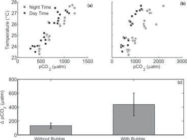
In the treatment experiment, we first tested for feed-backs in carbonate chemistry due to the presence of rub-ble: using a paired t test, we compared the day–night difference in measured pCO2 in each aquarium with
rubble, (pCO2,day−pCO2,night)rubble, and without rubble,
(pCO2,day−pCO2,night)no rubble.
Although we imposed four discrete temperature–pCO2
scenario treatments on each tank (Table 1), random varia-tion between treatments and the feedback between the rub-ble communities and the water chemistry resulted in near-continuous variation in temperature–pCO2treatments across
aquaria (Figs. 2 and S1 in the Supplement). To capture this continuous variation in temperature–pCO2 in the analysis,
we used the measured temperature–pCO2 seawater
condi-tion as a continuous independent variable in a regression rather than the four categorical treatment conditions in an ANOVA (an analysis ofGand NCP using the ANOVA ap-proach is included in Figs. S3, S4 and Tables S1, S2 in the Supplement). The regression approach allowed us to capture the quantitative relationships better between net calcifica-tion (G) or NCP and the temperature–pCO2treatment. We
created a single, continuous variable, standardized climate change (SCC), from a linear combination of temperature and pCO2values in each aquarium. A simple linear combination
was used becausepCO2increased linearly with temperature
Table 2. Regression results for the treatment experiments:Gday,
Gnight, and Gnetversus standardized climate change (Fig. 3a, c,
e) and NCPday, NCPnight, and NCPnetversus standardized climate
change (Fig. 3b, d, f). Bold values indicate a statistically significant
pvalue atα< 0.05.
SS df F p R2
Gday
Standardized climate change 3.79 1 1.45 0.06 (Standardized climate change)2 23.63 1 9.04 0.007
Error 54.89 21 0.33
Gnight
Standardized climate change 67.80 1 39.14 < 0.0001
Error 38.11 22 0.64
Gnet
Standardized climate change 88.01 1 19.49 < 0.001
Error 99.35 22 0.47
NCPday
Standardized climate change 5687.2 1 57.36 < 0.0001
Error 2181.4 22 0.72
NCPnight
Standardized climate change 3816.1 1 52.06 < 0.0001
Error 1612.6 22 0.70
NCPnet
Standardized climate change 17925 1 121.47 < 0.0001
Error 3246.4 22 0.85
using linear regression. The coefficients from this regression (slope: α=0.0031; y intercept: β= −0.078) were used to combine pCO2 and temperature onto the same scale, as a
measure of standardized climate change (Eq. 5):
1Tempi =Temptrt,i−Tempcont,i, (3) 1pCO2i=pCO2trt,i−pCO2cont,i, (4)
SCCi=1Tempi+α·1pCO2i+β. (5) This synthetic temperature–pCO2axis, SCC, is centered on
the ambient (control) conditions such that a value of 0 cor-responds to present-day Kaneohe Bay conditions, a nega-tive value corresponds to water that is colder and less acidic (pre-industrial) and a positive value corresponds to water that is warmer and more acidic (future conditions) compared to background seawater. (The independent relationships be-tweenG and NCP with1Temp and1pCO2 are shown in
Figs. S5 and S6 in the Supplement and are similar to the re-lationship with SCC.)
With SCC as a continuous, independent variable, we used a regression to test for linear and nonlinear relationships be-tween day, night, and net calcification (Gday, Gnight, and
Gnet)and NCP (NCPday, NCPnight, and NCPnet)versus SCC. For a simple test of nonlinearity in the response of calcifi-cation to SCC, we included a quadratic term (SCC2)in the
model. ForGday, we used weighted regression (weight
func-tion:wi=1/(1+|ri|)), wherewi=weight andri =residual, Fair, 1974) to account for heteroscedasticity. All other data met assumptions for a linear regression. Lastly, we used a linear regression to test the relationship betweenGand NCP.
0 500 1000 1500
23 24 25 26 27 28
pCO 2 (µatm)
Temperature (
°
C)
Night Time Day Time
0 1000 2000 3000
pCO 2 (µatm)
Without Rubble With Rubble
0 200 400 600 800
∆
pCO
2
(
µ
atm
)
(a) (b)
(c)
Figure 2.pCO2 and temperature in each aquarium (a) without any rubble present and(b)with rubble present. Daily variability in
pCO2was higher when rubble was present due to feedbacks from
the rubble community (note the differentxaxis scales in panels(a) and(b)). Panel(c)shows the mean difference between day and night
pCO2with and without rubble present, with observations paired by
aquarium (error bars are standard error) (t23= −7.23,p< 0.0001).
3 Results
3.1 Control experiment
For rubble in ambient seawater conditions, the average Gday, Gnight, and Gnet in the control experiment were 3.4±0.16 mmol m−2d−1, −2.4±0.15 mmol m−2d−1, and 0.96±0.20 mmol m−2d−1, respectively. There was no sig-nificant difference inGday (F3,23=0.68,p=0.58),Gnight (F3,23=1.52, p=0.24), or Gnet (F3,23=1.38, p=0.28) between racks in the control experiment (Fig. S2). NCP rates also did not show any rack effects. Average NCP rates were 23.2±1.4 mmol m−2d−1 (F3,23=0.07, p=0.94) during the day, −20.7±1.9 mmol m−2d−1 (F3,23=1.95, p=0.15) during the night, and 2.5±2.1 mmol m−2d−1 (F3,23=1.5,p=0.25) over the entire 24 h period.
3.2 Treatment experiment
The rubble communities significantly altered the seawater chemistry, with higher pCO2 than the applied pCO2
ma-nipulation, particularly at night (Fig. S1). The mean differ-ence between day and night pCO2 for all treatments was
−2 0 2 4 6
−10 −5
0
5 10
SCC
G net
0
5 10
G day
−10 −5
0
G night
−2 0 2 4 6
−100 −50 0 50 100
SCC
NCP
net
−50
0
50
NCP
day
−100 −50
0
NCP
night
Pre-IndustrialPresent2050 2100 Pre-IndustrialPresent2050 2100
x x x x x x
x x
Net Calc.
Net Diss.
Net Photo.
Net Resp.
(a) (b)
(c) (d)
(e) (f)
Figure 3.Net ecosystem calcification ((a)Gday,(c)Gnight,(e)and
Gnet)and net community production ((b)NCPday,(d)NCPnight,
and (f)NCPnet)versus standardized climate change (SCC). Each
point represents net ecosystem calcification (left panel) or net community production (right panel) calculated from an individual aquarium. Standardized climate change was centered around back-ground seawater conditions such that a value of 0 indicated that there was no change inpCO2or temperature. Positive values
indi-cate an elevatedpCO2and temperature condition relative to
back-ground, and negative values represent lower pCO2 and
tempera-ture conditions.Gday had a non-linear relationship with
standard-ized climate change (y= −0.27x2+ 0.59x+5.7), while Gnight
(y= −0.63x−3.6) andGnet(y= −0.76x+1.1) each had a
nega-tive linear relationship with standardized climate change (Table 2). NCPday (y= −7.01x+23.4), NCPnight (y= −35.76−4.74), and
NCPnet (y= −12.07x−10.85) all had significant negative
rela-tionships with standardized climate change. Black lines are best fit lines for each model with 95 % confidence intervals in gray. Thex’s in the top panel represent the imposed conditions for pre-industrial, present day, 2050, and 2100. The black horizontal line in panels(b), (e)and(f)shows the point whereGand NCP equal 0. Points above
the line are net calcifying(e)or net photosynthesizing(f)and points below the line are net dissolving(e)or net respiring(f)over the en-tire 24 h period.
Standardized climate change was a significant predictor forGday,Gnight, andGnet(Table 2; Fig. 3).Gdayhad a
non-linear relationship with standardized climate change (Ta-ble 2, Fig. 3a), increasing to a threshold and then rapidly declining. Gnight, however, had a strong linear relationship
−60 −40 −20 0 20 40 60
−20 −10 0 10 20
NCP mmol C m−2 d−1
G mmol CaCO
3
m
−2 d
−1 Day
Night
Standardized Climate Change
−2 0 2 4 6
1900 2000 2100 2200 2300
2100 2150 2200 2250 2300 2350
TA (
µ
mol kg
−1)
DIC (µmol kg−1)
Net Photosynthesis
Net Dissolution
Net Respiration
Net
Calcification
(a)
(b)
Figure 4. (a)CalculatedGand NCP rates for all treatment aquaria.
Squares are data collected during light (day) conditions and cir-cles represent data collected during dark (night) conditions, and the color represents standardized climate change (color bar). There is a strong positive relationship betweenGand NCP (y=0.14x+1.9,
p< 0.0001,R2=0.85). Negative and positiveyvalues are net dis-solution and net calcification, respectively; negative and positive
x values are net respiration and net photosynthesis, respectively.
(b)TA versus DIC: There is a strong positive relationship between TA and DIC (y= 0.31x+1577.4,p< 0.0001,R2=0.85). Black
and gray lines represent the best-fit line and 95 % confidence inter-vals, respectively. As expected, the slope of TA versus DIC (0.31) is approximately twice that ofGversus NCP (0.14).
with standardized climate change (Table 2; Fig. 3c), sug-gesting that joint increases in oceanpCO2and temperature
will increase nighttime dissolution of coral rubble. Lastly, Gnethad a strong negative relationship with standardized
cli-mate change (Table 2; Fig. 3e), and the rubble community switched from net calcification to net dissolution at an in-crease inpCO2 and temperature of 271 µatm and 0.75◦C,
respectively. Standardized climate change was also a signifi-cant predictor of NCP: day, night, and net NCP rates all de-clined with standardized climate change (Table 2; Fig. 3b, d, f).
Net ecosystem calcification increased with net commu-nity production (F1,46=260,p< 0.0001,R2=0.85; Fig. 4). In general, communities were net photosynthesizing and net calcifying during the day (Fig. 4a: squares in the upper right quadrant) and were net respiring and net dissolving at night (Fig. 4a: circles in the lower left quadrant). The exceptions were communities in the most extreme temperature–pCO2
4 Discussion
4.1 Carbonate chemistry feedbacks
The rubble communities in the aquaria significantly altered the seawater chemistry, particularly at night (t23= −7.23,
p< 0.0001; Figs. 2, S1). This day–night difference in seawa-ter chemistry increased under more extreme climate scenar-ios, as predicted by Jury et al. (2013). This large diel swing in pCO2is not uncommon in shallow coral reef environments.
pCO2ranged from 480 to 975 µatm over 24 h on a shallow
reef flat adjacent to our collection site (Silbiger et al., 2014) and from 450 to 742 µatm on a Moloka‘i reef flat dominated by coral rubble (Yates and Halley, 2006). Here,pCO2had
an average difference of 438 µatm between day and night, with a range of 412 µatm in the pre-industrial treatment to 854 µatm in the most extreme temperature–pCO2treatments
(Fig. 2). In our study, we incorporated these feedbacks into the statistical analysis by using the actual, sampled pCO2
(and temperature) in each aquarium (Fig. 3) rather than us-ing the intended pCO2 (and temperature) treatments in an
ANOVA (Tables S1, S2 and Figs. S3, S4), better reflecting thepCO2experienced by organisms in each aquarium.
4.2 Calcification, dissolution, and net community production in a high CO2and temperature
environment
Our results suggest that as pCO2 and temperature
in-crease over time, rubble reefs may shift from net calcifi-cation to net dissolution. In our study, this tipping point occurred at a pCO2 and temperature increase of 271 µatm
and 0.75◦C. Furthermore, our results showed that G
day
and Gnight in a natural coral rubble community have dif-ferent functional responses to changing pCO2 and
tem-perature (Fig. 3). The ranges in Gday and Gnight in our
aquaria were similar to in situ rates on Hawaiian rubble reefs. Yates and Halley (2006) saw Gday values between 3.3 and
11.7 mmol CaCO3m−2d−1andGnightvalues between−2.4
and−24 mmol CaCO3m−2d−1on a Moloka‘i reef flat with
coral rubble only (note that Yates and Halley calculated G over a 4 h time frame and that the data were multiplied by 3 here to showGin mmol m−2d−1). Also note that we normal-ized our rates to the surface area of the rubble, while Yates and Halley (2006) normalized their rates to planar surface area.).GdayandGnightin our experiment ranged from 1.9 to
9.4 and −1.3 to −10.5 mmol CaCO3m−2d−1, respectively,
across all treatment conditions. The higher dissolution rates in the in situ study by Yates and Halley (2006) are likely due to dissolution in the sediment, which was not present in our study.
Gday had a non-linear response to standardized
cli-mate change. Gday increased with temperature–pCO2until
slightly above ambient conditions, and then decreased un-der more extreme climate conditions (Fig. 3a). This mixed
response, increasing and then decreasing with standardized climate change, is reflected in prior experiments. We sug-gest three possible mechanisms to explain why calcification increases in slightly higher temperature–pCO2 than
ambi-ent conditions. (1) Some calcifiers can maintain and even in-crease their calcification rates in acidic conditions (Kamenos et al., 2013; Findlay et al., 2011; Rodolfo-Metalpa et al., 2011; Martin et al., 2013) by either modifying their local pH environment (Hurd et al., 2011) or partitioning their ener-getic resources towards calcification (Kamenos et al., 2013). For example, in low, stable pH conditions, the coralline al-gae,Lithothamnion glaciale, increased its calcification rate
relative to a control treatment, but did not concurrently in-crease its rate of photosynthesis (Kamenos et al., 2013). Ka-menos et al. (2013) suggest that the up-regulation of calci-fication may limit photosynthetic efficiency. In the present study, the increase inGday coincided with a decrease in net photosynthesis (Fig. 3a, b). Photosynthesizing calcifiers in the community may be partitioning their energetic resources more towards calcification and away from photosynthesis in order to maintain a positive calcification rate (Kamenos et al., 2013). Notably, turf algae likely have a major control over the NCP in this community, which would not have any impact on calcification. (2) An alternative hypothesis is that the calcifiers may be adapted or acclimatized to highpCO2
conditions (Johnson et al., 2014) and have not yet reached their threshold because the rubble was collected from a nat-urally high and variable pCO2 environment (Guadayol et
al., 2014; Silbiger et al., 2014). (3) In this study, the cal-cifiers experienced a combined increase in bothpCO2 and
temperature and, thus, the non-linear response inGdaymay
also be due a metabolic response. In a typical thermal perfor-mance curve, organisms increase their metabolism until they have reached a thermal maximum, and then rapidly decline (Huey and Kingsolver, 1989; Pörtner et al., 2006), and we see this response in our results. A recent study found a simi-lar non-linear response to temperature andpCO2in the coral Siderastrea sidera(Castillo et al., 2014). While they attribute
thepCO2response to photosynthesis being neutralized (we
did not see this response in our non-coral community), they suggest that the thermal response is due to both changes in metabolism and thermally driven changes in the aragonite saturation state (Castillo et al., 2014).
We saw a decline in both calcification and NCP in the extreme temperature–pCO2condition (Fig. 3). Calcification
has been shown to decline with climate stressors, and the magnitude of decline differs across species (Kroeker et al., 2010; Pandolfi et al., 2011; Ries et al., 2009; Kroeker et al., 2013). The concurrent decline in NCP and calcification (Figs. 3a, b and 4) suggests that non-photosynthesizing in-vertebrates in the community (such as bivalves) might be dominating the calcification signal in these conditions. This hypothesis would explain the pattern that we see in Fig. 4, where communities in the most extremepCO2and
maintaining a small, positive calcification rate (Fig. 4a: five points in the upper left quadrant).
Gnight rates are more straightforward, decreasing linearly withpCO2and temperature (Figs. 3c and 4). NCPnight rates
also decreased linearly withpCO2and temperature (Fig. 3d).
Similarly, Andersson et al. (2009) saw an increase in dissolu-tion under acidic condidissolu-tions in a community of corals, sand, and CCA. Previous studies on individual bioeroder taxa have also found higher rates of bioerosion or dissolution in more acidic, higher-temperature conditions (Wisshak et al., 2013; Fang et al., 2013; Reyes-Nivia et al., 2013; Tribollet et al., 2009; Wisshak et al., 2012). There are several mechanisms that could be mediating the increased dissolution rates in the high temperature–pCO2treatments. (1) Higher temperatures
could increase the metabolism of the bioeroder community, thus increasing borer activity (e.g., Davidson et al., 2013). (2) Because many boring organisms excrete acidic compounds to erode the skeletal structure (Hutchings, 1986), reduced pH in the overlaying water column may reduce the metabolic cost to the organisms, making it easier for eroders to break down the CaCO3. (3) Higher dissolution rates could be
medi-ated by an increase in the proportion of dolomite in the skele-tal structure of CCA on the rubble. A recent study found a 200 % increase in dolomite in CCA that were exposed to high pCO2and temperature conditions; this increase in dolomite
resulted in increased bioerosion by endolithic algae (Diaz-Pulido et al., 2014). However, it is unlikely that changes in the mineralogy of the CCA indirectly increased dissolution here, given the short timescale of our study. In the present study, we used the TA anomaly method to calculate chemical dissolution as a proxy for bioerosion. Future studies should also include measures of mechanical breakdown (e.g. the production of sponge chips) in addition to chemical disso-lution for a more complete picture of the impacts of climate stress on reef breakdown. Studies, including the present one, which focused on community-level responses, have consis-tently found that ocean acidification will increase dissolution rates on coral reefs (Andersson and Gledhill, 2013).
Standardized climate change explained more of the vari-ance in dissolution than in calcification in our rubble commu-nity (RG2night=0.64> RG2
day=0.33; Table 2). This result is
not surprising. Bioerosion, an important driver of dissolution, may be more sensitive to changes in ocean acidity than calci-fication, leading to net dissolution in high CO2waters. Many
boring organisms excrete acidic compounds, which may be less metabolically costly in a low pH environment. Erez et al. (2011) hypothesize that increased dissolution, rather than decreased calcification, maybe be the reason that net coral reef calcification is sensitive to ocean acidification. The re-sults of this study support this hypothesis. AlthoughGnet
de-clines linearly with temperature–pCO2, calcification (Gday) and dissolution (Gnight)have distinct responses to standard-ized climate change:Gday had a non-linear response, while Gnight declined linearly with standardized climate change.
Our results highlight the need to study the effects of climate stressors on both calcification and dissolution.
The Supplement related to this article is available online at doi:10.5194/bg-12-567-2015-supplement.
Author contributions. Conceived and designed the experiments: N. J. Silbiger, M. J. Donahue. Performed the experiments: N. J. Sil-biger. Analyzed the data: N. J. Silbiger, M. J. Donahue. Wrote the paper: N. J. Silbiger, M. J. Donahue.
Acknowledgements. Thanks to I. Caldwell, R. Coleman, J. Faith, K. Hurley, J. Miyano, R. Maguire, D. Schar, J. M. Sziklay, and M. M. Walton for help in field collections and lab analyses and to R. Briggs from UH SOEST Lab for Analytical Chemistry. M. J. Atkinson, R. Gates, C. Jury, H. Putnam, and R. Toonen gave thoughtful advice throughout the project. Comments by F. Macken-zie and our two anonymous reviewers improved this manuscript. This project was supported by a NOAA Nancy Foster Scholarship to N. J. Silbiger, a PADI Foundation Grant to N. J. Silbiger, and Hawaii SeaGrant 1847 to M. J. Donahue. This paper is funded in part by a grant/cooperative agreement from the National Oceanic and Atmospheric Administration, Project R/IR-18, which is sponsored by the University of Hawaii Sea Grant College Program, SOEST, under Institutional Grant No. NA09OAR4170060 from the NOAA Sea Grant Office, Department of Commerce. The views expressed herein are those of the author(s) and do not necessarily reflect the views of NOAA or any of its subagencies. This is HIMB contribution no. 1607, Hawaii SeaGrant contribution no. UNIHI-SEAGRANT-JC-12-19, and SOEST contribution no. 9237.
Edited by: J. Middelburg
References
Adey, W. H.: Review – coral reefs: algal structures and mediated ecosystems in shallow turbulent, alkaline waters, J. Phycol., 34, 393–406, 1998.
Andersson, A. J. and Gledhill, D.: Ocean Acidification and Coral Reefs: Effects on Breakdown, Dissolution, and Net Ecosystem Calcification, Ann. Rev. Mar. Sci., 5, 321–348, 2013.
Andersson, A. J. and Mackenzie, F. T.: Revisiting four scientific debates in ocean acidification research, Biogeosciences, 9, 893– 905, doi:10.5194/bg-9-893-2012, 2012.
Andersson, A. J., Kuffner, I. B., Mackenzie, F. T., Jokiel, P. L., Rodgers, K. S., and Tan, A.: Net Loss of CaCO3 from a subtropical calcifying community due to seawater acidifica-tion: mesocosm-scale experimental evidence, Biogeosciences, 6, 1811–1823, doi:10.5194/bg-6-1811-2009, 2009.
Bopp, L., Resplandy, L., Orr, J. C., Doney, S. C., Dunne, J. P., Gehlen, M., Halloran, P., Heinze, C., Ilyina, T., Séférian, R., Tjiputra, J., and Vichi, M.: Multiple stressors of ocean ecosys-tems in the 21st century: projections with CMIP5 models, Biogeosciences, 10, 6225–6245, doi:10.5194/bg-10-6225-2013, 2013.
Caldeira, K. and Wickett, M. E.: Oceanography: anthropogenic car-bon and ocean pH, Nature, 425, 365–365, 2003.
Camoin, G. F. and Montaggioni, L. F.: High energy coralgal-stromatolite frameworks from Holocene reefs (Tahiti, French Polynesia), Sedimentology, 41, 656–676, 1994.
Castillo, K. D., Ries, J. B., Bruno, J. F., and Westfield, I. T.: The reef-building coralSiderastrea sidereaexhibits parabolic re-sponses to ocean acidification and warming, Proc. R. Soc. B., 281, 20141856, 2014.
Comeau, S., Edmunds, P. J., Spindel, N. B., and Carpenter, R. C.: The responses of eight coral reef calcifiers to increasing par-tial pressure of CO2 do not exhibit a tipping point, Limnol. Oceanogr, 58, 388–398, 2013.
Cubasch, U., Wuebbles, D., Chen, D., Facchini, M. C., Frame, D., Mahowald, N., and Winther, J.-G.: Climate Change 2013: The Physical Science Basis, Contribution of Working Group I to the Fifth Assessment Report of the Intergovernmental Panel on Cli-mate Change Cambridge, United Kingdom and New York, NY, USA, 119–158, 2013.
Davidson, T. M., de Rivera, C. E., and Carlton, J. T.: Small increases in temperature exacerbate the erosive effects of a non-native bur-rowing crustacean, J. Exp. Mar. Biol. Ecol., 446, 115–121, 2013. Diaz-Pulido, G., Anthony, K., Kline, D. I., Dove, S., and Hoegh-Guldberg, O.: Interactions between ocean acidification and warming on the mortality and dissolution of coralline alge, J. Phycol., 48, 32–39, 2012.
Diaz-Pulido, G., Nash, M. C., Anthony, K. R. N., Bender. D., Opdyke, B. N., Reyed-Nivia, C., and Troitzsch, U.: Greenhouse conditions induce mineralogical changes and dolomite accumu-lation in coralline algae on tropical reefs, Nature Communica-tions, 5, 3310, doi:10.1038/ncomms4310, 2014.
Dickson, A. G.: Standard potential of the reaction: AgCl (s)+
12H2(g)=Ag (s)+HCl (aq), and and the standard acidity
con-stant of the ion HSO−
4 in synthetic sea water from 273.15 to
318.15 K, J. Chem. Thermodyn., 22, 113–127, 1990.
Dickson, A. G. and Millero, F. J.: A comparison of the equilibrium constants for the dissociation of carbonic acid in seawater media, Deep-Sea Res.-Pt. I, 34, 1733–1743, 1987.
Dickson, A. G., Sabine, C. L., and Christian, J. R.: Guide to best practices for ocean CO2 measurements, Sidney, British Columbia, North Pacific Marine Science Organization, PICES Special Publication 3, 2007.
Doney, S. C., Fabry, V. J., Feely, R. A., and Kleypas, J. A.: Ocean Acidification: The Other CO2Problem, Ann. Rev. Mar. Sci., 1, 169–192, 2009.
Drupp, P. S., De Carlo, E. H., Mackenzie, F. T., Sabine, C. L., Feely, R. A., and Shamberger, K. E.: Comparison of CO2dynamics
and air–sea gas exchange in differing tropical reef environments, Aquat. Geochem., 19, 371–397, 2013.
Erez, J., Reynaud, S., Silverman, J., Schneider, K., and Allemand, D.: Coral calcification under ocean acidification and global change, in: Coral Reefs: an ecosystem in transition, edited by: Dubinski, Z. and Stambler, N., Springer, 151–176, 2011.
Fabricius, K. E.: Effects of terrestrial runoff on the ecology of corals and coral reefs: review and synthesis, Mar. Pollut. Bull., 50, 125– 146, 2005.
Fabricius, K., Langdon, C., Uthicke, S., Humphrey, C., Noonan, S., De’ath, G., Okazaki, R., Muehllehner, N., Glas, M., and Lough, J.: Losers and winners in coral reefs acclimatized to elevated car-bon dioxide concentrations, Nature Climate Change, 1, 165–169, 2011.
Fair, R. C.: On the robust estimation of econometric models, in: Annals of Economic and Social Measurement, 3, NBER, 117– 128, 1974.
Fang, J. K. H., Mello-Athayde, M. A., Schönberg, C. H. L., Kline, D. I., Hoegh-Guldberg, O., and Dove, S.: Sponge biomass and bioerosion rates increase under ocean warming and acidification, Glob. Change Biol., 19, 3581–3591, 2013.
Fangue, N. A., O’Donnell, M. J., Sewell, M. A., Matson, P. G., MacPherson, A. C., and Hofmann, G. E.: A laboratory-based, experimental system for the study of ocean acidification effects on marine invertebrate larvae, Limnol. Oceanogr.-Meth., 8, 441– 452, 2010.
Feely, R. A., Sabine, C. L., Lee, K., Berelson, W., Kleypas, J., Fabry, V. J., and Millero, F. J.: Impact of anthropogenic CO2 on the CaCO3system in the oceans, Science, 305, 362–366, 2004. Findlay, H. S., Wood, H. L., Kendall, M. A., Spicer, J. I., Twitchett,
R. J., and Widdicombe, S.: Comparing the impact of high CO2 on calcium carbonate structures in different marine organisms, Mar. Biol. Res., 7, 565–575, 2011.
Gattuso, J.-P., Frankignoulle, M., and Smith, S. V.: Measurement of community metabolism and significance in the coral reef CO2 source-sink debate, Proc. Natl. Acad. Sci., 96, 13017–13022, 1999.
Guadayol, Ò., Silbiger, N. J., Donahue, M. J., and Thomas, F. I. M.: Patterns in Temporal Variability of Temperature, Oxygen and pH along an Environmental Gradient in a Coral Reef, PloS one, 9, e85213, doi:10.1371/journal.pone.0085213, 2014.
Harrington, L., Fabricius, K., De’ath, G., and Negri, A.: Recog-nition and selection of settlement substrata determine post-settlement survival in corals, Ecology, 84, 3428–3437, 2004. Hoegh-Guldberg, O., Mumby, P. J., Hooten, A. J., Steneck, R. S.,
Greenfield, P., Gomez, E., Harvell, C. D., Sale, P. F., Edwards, A. J., Caldeira, K., Knowlton, N., Eakin, C. M., Iglesias-Prieto, R., Muthiga, N., Bradbury, R. H., Dubi, A., and Hatziolos, M. E.: Coral reefs under rapid climate change and ocean acidification, Science, 318, 1737–1742, 2007.
Huey, R. B. and Kingsolver, J. G.: Evolution of thermal sensitivity of ecotherm performance, Trends Ecol. Evol., 4, 131–135, 1989. Hutchings, P. A.: Biological destruction of coral reefs, Coral Reefs,
4, 239–252, 1986.
Hoegh-Guldberg, O. and Bruno, J. F.: The impact of climate change on the world’s marine ecosystems, Science, 328, 1523–1528, 2010.
Hurd, C. L., Cornwall, C. E., Currie, K., Hepburn, C. D., McGraw, C. M., Hunter, K. A., and Boyd, P. W.: Metabolically induced pH fluctuations by some coastal calcifiers exceed projected 22nd century ocean acidification: a mechanism for differential suscep-tibility?, Glob. Change Biol., 17, 3254–3262, 2011.
Hy-drolithon onkodesand increase susceptibility to grazing, J. Exp. Mar. Biol. Ecol., 434, 94–101, 2012.
Johnson, M. D., Moriarty, V. W., and Carpenter, R. C.: Ac-climatization of the Crustose Coralline Alga Porolithon onkodes to Variable pCO2, PLOS ONE, 9, e87678,
doi:10.1371/journal.pone.0087678, 2014.
Jokiel, P. L., Rodgers, K. S., Kuffner, I. B., Andersson, A. J., Cox, E. F., and Mackenzie, F. T.: Ocean acidification and calcifying reef organisms: a mesocosm investigation, Coral Reefs, 27, 473–483, 2008.
Jury, C. P., Thomas, F. I. M., Atkinson, M. J., and Toonen, R. J.: Buffer Capacity, Ecosystem Feedbacks, and Seawater Chemistry under Global Change, Water, 5, 1303–1325, 2013.
Kamenos, N. A., Burdett, H. L., Aloisio, E., Findlay, H. S., Mar-tin, S., Longbone, C., Dunn, J., Widdicombe, S., and Calosi, P.: Coralline algal structure is more sensitive to rate, rather than the magnitude, of ocean acidification, Glob. Change Biol., 19, 3621– 3628, 2013.
Kleypas, J. and Langdon, C.: Coral reefs and changing seawater chemistry, in: Coral Reefs and Climate Change: Science and Managemen., edited by: Phinney, J., Skirving, W., Kleypas, J., and Hoegh-Guldberg, O., American Geophysical Union, Wash-ington D.C., 73–110, 2006.
Kroeker, K. J., Kordas, R. L., Crim, R. N., and Singh, G. G.: Meta-analysis reveals negative yet variable effects of ocean acidifica-tion on marine organisms, Ecol. Lett., 13, 1419–1434, 2010. Kroeker, K. J., Kordas, R. L., Crim, R., Hendriks, I. E., Ramajo, L.,
Singh, G. S., Duarte, C. M., and Gattuso, J. P.: Impacts of ocean acidification on marine organisms: quantifying sensitivities and interaction with warming, Glob. Change Biol., 19, 1884–1896, 2013.
Littler, M. M.: The population and community structure of Hawai-ian fringing-reef crustose corallinaceae (Rhodophyta, Cryptone-miales), J. Exp. Mar. Biol. Ecol., 11, 103–120, 1973.
Lowe, R. J., Falter, J. L., Monismith, S. G., and Atkin-son, M. J.: A numerical study of circulation in a coastal reef-lagoon system, J. Geophys. Res.-Oceans, 114, C06022, doi:10.1029/2008JC005081, 2009a.
Lowe, R. J., Falter, J. L., Monismith, S. G., and Atkinson, M. J.: Wave-driven circulation of a coastal reef-lagoon system, J. Phys. Oceanogr., 39, 873–893, 2009b.
Martin, S., Cohu, S., Vignot, C., Zimmerman, G., and Gattuso, J. P.: One-year experiment on the physiological response of the Mediterranean crustose coralline alga,Lithophyllum cabiochae, to elevated pCO2 and temperature, Ecol. Evol., 3, 676–693,
doi:10.1029/2008JC005081, 2013.
Mehrbach, C.: Measurement of the apparent dissociation constants of carbonic acid in seawater at atmospheric pressure, Limnol. Oceanogr., 18, 897–907, 1973.
Meinshausen, M., Smith, S. J., Calvin, K., Daniel, J. S., Kainuma, M. L. T., Lamarque, J. F., Matsumoto, K., Montzka, S. A., Raper, S. C. B., and Riahi, K.: The RCP greenhouse gas concentrations and their extensions from 1765 to 2300, Clim. Change, 109, 213– 241, 2011.
Pandolfi, J. M., Connolly, S. R., Marshall, D. J., and Cohen, A. L.: Projecting coral reef futures under global warming and ocean acidification, Science, 333, 418–422, 2011.
Price, N.: Habitat selection, facilitation, and biotic settlement cues affect distribution and performance of coral recruits in French Polynesia, Oecologia, 163, 747–758, 2010.
Pörtner, H. O., Bennet, A. F., Bozinovic, F., Clarke, A., Lardies, M. A., Lucassen, M., Pelster, B., Schiemer, F., and Stillman, J. H.: Trade-offs in therman adaptation: the need for molecular ecolog-ical integration, Phys. Biochem. Zool., 79, 295–313, 2006. Putnam, H. M.: Resilience and acclimatization potential of reef
corals under predicted climate change stressors, PhD, Zoology, University of Hawaii at Manoa, Honolulu, 1–154, 2012. Reyes-Nivia, C., Diaz-Pulido, G., Kline, D., Guldberg, O.-H., and
Dove, S.: Ocean acidification and warming scenarios increase microbioerosion of coral skeletons, Glob. Change Biol., 19, 1919–1929, 2013.
Ries, J. B., Cohen, A. L., and McCorkle, D. C.: Marine calcifiers exhibit mixed responses to CO2-induced ocean acidification, Ge-ology, 37, 1131–1134, 2009.
Rodolfo-Metalpa, R., Houlbrèque, F., Tambutté, É., Boisson, F., Baggini, C., Patti, F. P., Jeffree, R., Fine, M., Foggo, A., and Gattuso, J. P.: Coral and mollusc resistance to ocean acidifica-tion adversely affected by warming, Nature Climate Change, 1, 308–312, 2011.
Rogelj, J., Meinshausen, M., and Knutti, R.: Global warming un-der old and new scenarios using IPCC climate sensitivity range estimates, Nature Climate Change, 2, 248–253, 2012.
Sanford, T., Frumhoff, P. C., Luers, A., and Gulledge, J.: The cli-mate policy narrative for a dangerously warming world, Nature Climate Change, 4, 164–166, 2014.
Semesi, I. S., Kangwe, J., and Björk, M.: Alterations in seawater pH and CO2affect calcification and photosynthesis in the tropical coralline alga,Hydrolithonsp. (Rhodophyta), Estuarine, Coast. Shelf Sci., 84, 337–341, 2009.
Silbiger, N., Guadayol, Ò., Thomas, F. I. M., and Donahue, M.: Reefs shift from net accretion to net erosion along a natural en-vironmental gradient, Mar. Ecol. Prog. Ser., 515, 33–44, 2014. Smith, S. V. and Key, G. S.: Carbon dioxide and metabolism in
ma-rine environments, Limnol. Oceanogr, 20, 493–495, 1975. Smith, S. V., Kimmerer, W. J., Laws, E. A., Brock, R. E., and Walsh,
T. W.: Kaneohe Bay sewage diversion experiment – perspectives on ecosystem responses to nutritional perturbation, Pacific Sci-ence, 35, 279–402, 1981.
Solomon, S., Qin. D., Manning. M. Chen. Z., Marquis, M., Bindoff, N. L., Willebrand, J., Artale, V., Cazenave, A., Gregory, J., Gulev, S., Hanawa, K., Le Quéré, C., Levitus, S., Nojiri, Y., Shum, C. K., Talley L. D., and Unnikrishnan, A.: Observations: Oceanic Climate Change and Sea Level, in: Climate Change 2007: The Physical Science Basis, Contribution of Working Group I to the Fourth Assessment Report of the Intergovernmental Panel on Climate Change, edited by: Solomon, S., Qin, D., Manning, M., Chen, Z., Marquis, M., Averyt, K. B., Tignor, M., and Miller, H. L., Cambridge University Press, Cambridge, United Kingdom and New York, NY, USA, 387–429, 2007.
Stimson, J. and Kinzie III, R. A.: The temporal pattern and rate of release of zooxanthellae from the reef coralPocillopora dami-cornis(Linnaeus) under nitrogen-enrichment and control condi-tions, J. Exp. Mar. Biol. Ecol., 153, 63–74, 1991.
Tribollet, A. and Payri, C.: Bioerosion of the coralline alga Hy-drolithon onkodesby microborers in the coral reefs of Moorea, French Polynesia, Oceanol. Acta, 24, 329–342, 2001.
Tribollet, A., Atkinson, M. J., and Langdon, C.: Effects of elevated
pCO(2)on epilithic and endolithic metabolism of reef
carbon-ates, Glob. Change Biol., 12, 2200–2208, 2006.
Tribollet, A., Godinot, C., Atkinson, M., and Langdon, C.: Ef-fects of elevated pCO(2) on dissolution of coral carbonates by microbial euendoliths, Glob. Biogeochem. Cy., 23, GB3008, doi:10.1029/2008GB003286, 2009.
Uppström, L. R.: The boron/chlorinity ratio of deep-sea water from the Pacific Ocean, Deep-Sea Res., 21, 161–162, 1974.
Van Heuven, S., Pierrot, D., Lewis, E., and Wallace, D. W. R.: MATLAB Program developed for CO2system calculations, Rep. ORNL/CDIAC-105b, 2009.
van Heuven, S., Pierrot, D., Rae, J. W. B., Lewis, E., and Wal-lace, D. W. R.: 5 MATLAB program developed for CO2system
calculations, ORNL/CDIAC-105b, Carbon Dioxide Inf. Anal. Cent., Oak Ridge Natl. Lab., US DOE, Oak Ridge, Tenn., doi:10.3334/CDIAC/otg.CO2SYS_MATLAB_v1.1, 2011. Van Vuuren, D. P., Meinshausen, M., Plattner, G. K., Joos, F.,
Strassmann, K. M., Smith, S. J., Wigley, T. M. L., Raper, S. C. B., Riahi, K., and De La Chesnaye, F.: Temperature increase of 21st century mitigation scenarios, Proc. Natl. Acad. Sci., 105, 15258–15262, 2008.
Van Vuuren, D. P., Edmonds, J., Kainuma, M., Riahi, K., Thomson, A., Hibbard, K., Hurtt, G. C., Kram, T., Krey, V., and Lamarque, J.-F.: The representative concentration pathways: an overview, Clim. Change, 109, 5–31, 2011.
White, J.: Distribution, recruitment and development of the borer community in dead coral on shallow Hawaiian reefs, Ph.D., Zo-ology, University of Hawaii at Manoa, Honolulu, 1980. Wisshak, M., Schönberg, C. H. L., Form, A., and Freiwald, A.:
Ocean acidification accelerates reef bioerosion, Plos One, 7, e45124, doi:10.1371/journal.pone.0045124, 2012.
Wisshak, M., Schönberg, C. H. L., Form, A., and Freiwald, A.: Ef-fects of ocean acidification and global warming on reef bioero-sion – lessons from a clionaid sponge, Aquat. Biol., 19, 111–127, 2013.
Wolf-Gladrow, D. A., Zeebe, R. E., Klass, C., Körtzinger, A., and Dickson, A. G.: Total Alkalinity: The explicit conservative ex-pression and its application to biogeochemical processes, Mar. Chem., 106, 287–300, 2007.
Yates, K. K. and Halley, R. B.: CO2−
3 concentration and pCO2