Confidence in Phase Definition for Periodicity in Genes Expression Time Series.

(1)

Confidence in Phase Definition for Periodicity

in Genes Expression Time Series

Mohammed El Anbari*, Abeer Fadda, Andrey Ptitsyn

Division of Biomedical Informatics, Sidra Medical and Research Center, Doha, Qatar

Abstract

Circadian oscillation in baseline gene expression plays an important role in the regulation of multiple cellular processes. Most of the knowledge of circadian gene expression is based on studies measuring gene expression over time. Our ability to dissect molecular events in time is determined by the sampling frequency of such experiments. However, the real peaks of gene activity can be at any time on or between the time points at which samples are collected. Thus, some genes with a peak activity near the observation point have their phase of oscillation detected with better precision then those which peak between observa-tion time points. Separating genes for which we can confidently identify peak activity from ambiguous genes can improve the analysis of time series gene expression. In this study we propose a new statistical method to quantify the phase confidence of circadian genes. The numerical performance of the proposed method has been tested using three real gene expression data sets.

Introduction

Analysis of periodic patterns is an essential part of many studies of gene expression involving timeline sampling or targeting of rhythmically expressed genes. Recent publications report a large proportion of the entire transcriptome oscillating in a circadian (i.e. approximately daily) rhythm [1–3]. The number of genes for which circadian baseline can be identified as statisti-cally significant over stochastic noise is traditionally thought to be under 10% [4–6], but more recently estimated as 43% [1] or even close to 100% [7], depending on the algorithms applied. Significance of the signal-to-noise ratio is the focus of most studies targeting rhythmic expres-sion. The absolute amplitude and time of the peak (i.e. phase) of rhythmic gene expression are also analyzed and reported. However, we feel that one aspect of rhythmic gene expression required additional consideration. It has been observed that low sampling frequency presents a significant challenge to all studies of periodic gene expression ([7] for review). Most gene expression studies only report 6 or 9 observation points per period and not more than two con-secutive periods in the entire timeline. Some oscillating genes may have peak expression coin-ciding at, or near, the observation point (i.e. the time when the animal is sacrificed and tissue samples are taken for analysis). However, other genes may peak at any time between sparsely placed observations. Since our ability to differentiate events in time is restricted by the low

a11111

OPEN ACCESS

Citation:El Anbari M, Fadda A, Ptitsyn A (2015) Confidence in Phase Definition for Periodicity in Genes Expression Time Series. PLoS ONE 10(7): e0131111. doi:10.1371/journal.pone.0131111

Editor:Ying Xu, University of Georgia, UNITED STATES

Received:January 13, 2015

Accepted:May 28, 2015

Published:July 10, 2015

Copyright:© 2015 El Anbari et al. This is an open access article distributed under the terms of the Creative Commons Attribution License, which permits unrestricted use, distribution, and reproduction in any medium, provided the original author and source are credited.

Data Availability Statement:All relevant data are within the paper and its Supporting Information files.

Funding:The authors have no support or funding to report.

(2)

it be possible to make a quantitative estimation of confidence that a gene peaks at a certain time of the day? With such a metric we could separate a fraction of genes for which we know the true time of peak and analyze the function of genes at a given time with less noise (i.e. genes highly expressed, but peaking at a different time) mixed in. To answer these questions and enable time-wise analysis of gene function and interactions, we propose a novel algorithm for the estimation of confidence of phase assignment in analysis to timeline expression profiles.

To answer the questions posed for this study we propose to use the bootstrap, which is a general technique for estimating unknown quantities associated with statistical models. Often the bootstrap is used to find

• standard errors for estimators,

• confidence intervals for unknown parameters,

• p-values for test statistics under a null hypothesis.

The maximum entropy bootstrap [8] is a resampling method for observations that are not nec-essarily independent and/or identically distributed. These conditions match typical observa-tions of gene expressions time series. The maximum entropy bootstrap is an algorithm that constructs a large number of replicates (such asR= 999) that retain the basic shape, local peaks and troughs and time independence of the original time series, by being strongly dependent on it. The maximum entropy bootstrap is particularly useful for short time series.

Materials and Methods

Notations

I: indicator function.

n: the sample size.

p: the number of genes.

χ= {X1,. . .,Xn}: random sample from population.

w_{¼ f}_X 1; :::;X

ng: resample obtained by sampling fromχ.

α: level of confidence.

^

y: estimate ofθ, computed fromχ.

^

y_{: bootstrap version of}_y^_{, computed from}_χ_.

Phase estimation

We consider a gene expression time series {x1,. . .,xn}. Without loss of generality, suppose that

the measurements are taken in time pointst= 0, 4, 8,. . ., 44h. We can then construct a collec-tion of intervals namedphasesand labeledG0,G1,. . .,G5such that

G0 ¼ ½ 2;2;G1 ¼ ½2;6;G2¼ ½6;10;G3¼ ½10;14;G4¼ ½14;18;G5 ¼ ½18;22: ð1Þ

Letθbe theﬁrstpeak timeor thephaseof the gene expression. We are interested inestimating

and in a later stepconstructing a conﬁdence intervalforθ. More precisely, we want to construct an interval contained in one of the classesGi, and that contains the estimated parametery^with

high probability.

(3)

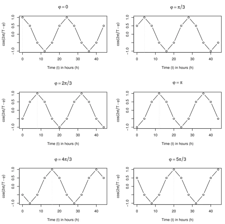
1. Generate 6 cosine waves with the equation given below

C

φðtÞ ¼ cos 2p

T t φ

;t¼0;4;8; :::;44;φ2 f0;p=3;2p=3;p;4p=3;5p=3g: ð2Þ

The following properties apply: the periods are 24h, 48h long (two cycles), and the intervals between adjacent phases is 4h.Fig 1is a graphical representation of the cosine (Eq 2).

2. Calculate the correlation coefficient between the gene expression profile and each of the 6 cosine wavesC_φ_{. Let}R¼ fr0^ ;^r1; :::;r5^ gdenotes the obtained vector of correlations. Let

^

r ¼ maxR; ð3Þ

be the highest correlation andφ^the phase of the corresponding cosine wave. The optimal C_^

φis selected to be the representative of the circadian rhythmicity if the correlation is

sig-niﬁcant. Our parameter of interestθis then estimated by the peak of thebest-correlated

cosine curve, and it is equal to

^

y¼φT=^ 2p¼12^φ=p: ð4Þ

Data resampling using Maximum Entropy Bootstrap Algorithm

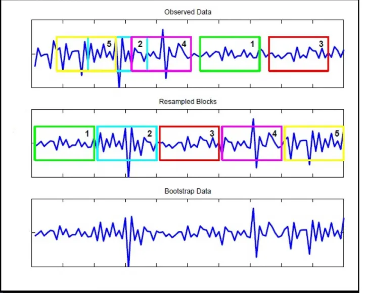
Several bootstrap methods have been proposed for time series data. The most well-known is theMoving Block Bootstrap. This procedure works by dividing the observations in blocks of lengthband then resampling the blocks (SeeFig 2for an illustration). The main problem with the block bootstrap is that the block length,b, which is a form of smoothing parameter, needs to be chosen. If the blocks are too short, the bootstrap samples cannot mimic the original sam-ple. In this case dependency is broken whenever we start a new block. If, on the other hand, the blocks are too long, we will lose the randomness of the replicates. For these reasons, in this study we apply the maximum entropy bootstrap algorithm proposed by [8]. It does not impose strong assumptions on the distribution of the time series like stationarity. A full description of the algorithm can be found in [9]. The replications are generated by the following steps

1. Form order statisticsx(t)by sorting increasingly the original data, and keep the vector of

ordering index.

2. Using the ordering statistics obtained at step 1, compute the intermediate pointsz(t)=

(x(t)+x(t+1))/2 fort= 1,. . .,n−1.

3. Fort= 1,. . .,n, construct the deviationx(t)−x(t−1), and calculate the trimmed meanmtrm

of the obtained observations. The lower limit for left tail isz0=x(1)−mtrmand upper limit

for right tail iszn=x(n)+mtrm.z0andznare the new limiting intermediate points.

4. Compute the mean of the maximum entropy (ME) density within each interval while satis-fying themean-preserving constraint.

5. Generate uniformly distributed numbers on the [0, 1] interval, then calculate sample quan-tiles of the Maximum Entropy at the generated points and sort them.

6. Using the ordering index of step 1, reorder the sorted sample. This process permits to con-serve the dependance relationships among observations in the original data.

(4)

0 10 20 30 40

−1.0

0.0

0.5

1.0

ϕ =0

Time (t) in hours (h)

cos ( 2 π t T −ϕ )

0 10 20 30 40

−1.0

0.0

0.5

1.0

ϕ = π 3

cos ( 2 π t T −ϕ )

0 10 20 30 40

−1.0

0.0

0.5

1.0

ϕ =2π 3

cos ( 2 π t T −ϕ )

0 10 20 30 40

−1.0

0.0

0.5

1.0

ϕ = π

cos ( 2 π t T −ϕ )

0 10 20 30 40

−1.0

0.0

0.5

1.0

ϕ =4π 3

cos ( 2 π t T −ϕ )

0 10 20 30 40

−1.0

0.0

0.5

1.0

ϕ =5π 3

cos ( 2 π t T −ϕ )

Fig 1. Graph of the ideal cosines.Graph representing the cosine waves:cosð2p

Tt φÞfort= 0,4,8,. . ., 44 andφ2{0,π/3, 2π/3,π, 5π/3}. The dotted vertical line shows theﬁrstpeak time.

(5)

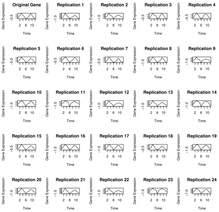
A complete simulated example for illustration of each step of the algorithm can be found in [9].Fig 3shows one gene expression time series from the IWAT data, along with 24 different replicates of the series chosen randomly from 999 used in the analysis. Due to the fact that the maximum entropy algorithm tries to retain all the properties of the data, one can see that the replicates remain close to the original time series.

The Bootstrap Approach for

p

-value

Let^tdenote the realized value of a test statisticτcomputed for a particular sample. Then

P_ð_t_^_t_j_H

0Þis the deﬁnition of thep-value in situations where large values ofτsupport the alternative hypothesis. The process of calculatingp-value consists of the following steps:

1. Specify a way to generate bootstrap samples that resemble the real data while satisfying the null hypothesisH0. In our case we will use theMaximum Entropy Bootstrap Algorithm.

2. LetMEBAdenote thisbootstrap data-generating process.

Fig 2. Graph of the moving block bootstrap principle.Graph showing the principal of moving block bootstrap. The moving block bootstrap randomly selects blocks of the original data (top) and concatenate them together (center) to form a resample (bottom).

(6)

2 6 10

−0.5

Original Gene

Time

Gene Expression 2 6 10

−1.0

Replication 1

Time

−1.0

Replication 2

Time

−0.5

Replication 3

Time

−0.5

Replication 4

Time

Gene Expression

2 6 10

−0.5

Replication 5

Time

−0.5

Replication 6

Time

−0.5

Replication 7

Time

−1.0

Replication 8

Time

−1.0

Replication 9

Time

Gene Expression

2 6 10

−1.0

Replication 10

Time

−1.0

Replication 11

Time

−1.0

Replication 12

Time

−1.0

Replication 13

Time

−1.0

Replication 14

Time

Gene Expression

2 6 10

−0.5

Replication 15

Time

−1.0

Replication 16

Time

−1.0

Replication 17

Time

−0.5

Replication 18

Time

−1.0

Replication 19

Time

Gene Expression

2 6 10

−1.0

Replication 20

Time

−1.0

Replication 21

Time

−1.0

Replication 22

Time

−1.0

Replication 23

Time

−1.0

Replication 24

Time

Gene Expression

Fig 3. An Example of data resampling using the Maximum Entropy Bootstrap Algorithm.(Top left panel): A gene expression time series from the IWAT data. (Remaining:) Set of 24 replications randomly chosen from 999 maximum entropy bootstrap samples used in the analysis.

(7)

3. UsingMEBA, generateR= 999 bootstrap samples indexed byj. From each of them, com-pute a bootstrap test statistict_j. To estimate a bootstrapp-value, we use

^

p_ð_^_t_{Þ ¼}

1þPR

j¼1Ift j>^tg

1þR :

ð5Þ

Arguments in favor of the latter formulae for calculatingp-value instead of the classical for-mulaePR

j¼1Ift j>^tg

=R, can be found in [10], p. 148, 161). For example, if 73 of thet_j are

greater than^t, then_p^ð^tÞ ¼ ð1þ73Þ=ð1þ999Þ ¼0:074.

4. Reject the null hypothesisH0if^pð^tÞ<a. Whereαis a given constant satisfying 0<α<1.

In general we takeα= 0.05.

This algorithm will be used to assess significance of the correlation between a gene expres-sion time series and one of the cosine (Eq 2).

Bootstrap Percentile Confidence Interval

The main focus of this paper is to give an accurate approximate confidence interval forpeak timeparameter^y. Computing such confidence intervals with distributions that are difficult to represent mathematically, is very challenging. The bootstrap is another class of general meth-ods for constructing confidence intervals without making strong distributional assumptions about the data or the statistic being calculated. There are several ways to construct bootstrap confidence intervals. They vary in ease of calculation and accuracy. There have been three main lines of development: Efron’s original percentile method [11], the bootstraptinterval introduced in [12], and the double bootstrap interval introduced in [13]. In this work, due to its simplicity and good performance, we use the Bootstrap Percentile Confidence Interval.

Let^ybe an estimator ofθon the measured dataX1,. . .,Xn, andy^be its analog on a

boot-strapped sampleX 1; :::;X

n, then:

KbootðxÞ ¼Pðfy^ xgÞ: ð6Þ

WhereKbootis the empirical distribution function of the bootstrap values. Efron’s (1979)

origi-nal 100(1−2α)% bootstrappercentile intervalis to just take the empirical 100αand 100(1−α)

percentiles from the bootstrap values^y 1; :::;y^

R. Then the 100(1−2α)% percentile interval is

½y_bp;y_bp ¼ ½K 1

bootðaÞ;K

1

bootð1 aÞ; ð7Þ

whereK 1

bootis the inverse or the generalized inverse distribution function or quantile function. The name percentile comes from the fact thatK 1

bootðaÞandK 1

bootð1 aÞare percentiles of the bootstrap distributionKbootin (Eq 6). In practice, we proceed as follows:

1. GenerateRbootstrap samples of sizenusing the maximum entropy algorithm.

2. Estimate the parameterθof interest for each bootstrap sample:^y_bforb= 1,. . .,R.

3. Order the bootstrap replications of^ysuch that^y_ð₁_Þy^_ð₂_Þ:::^y_ð_R_Þ. The lower and upper confidence bounds are theR.αthandR.(1−α)thordered elements, respectively. The esti-mated (1−2α) confidence interval ofy^is

½y_bp;y_bp ¼ ½^y ðR:aÞ;y^

(8)

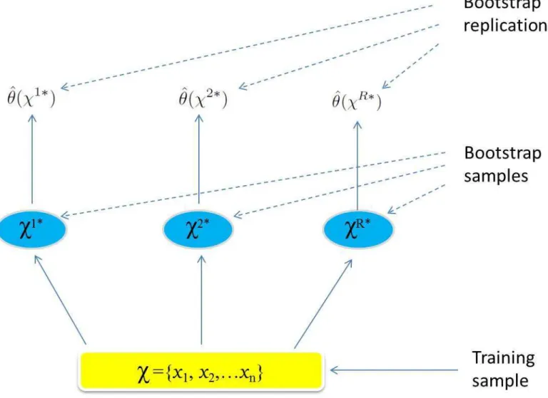
Fig 4summarizes the steps of the Bootstrap Percentile confidence interval principle.

Remark 1. IfR.αis not an integer, the following procedure can be used:

Letk= [(R+ 1)α], the largest integer(R+ 1)α. Then we define the empiricalαand (1−

α) quantities by thekthlargest and (R+k−1)thvalues ofy^ðbÞ, respectively. So ifR= 999 andα = 2.5% these are the 25thand 975thordered elements.

We have now all the pieces needed to accomplish the phase confidence analysis. Algorithm 1 summarizes the details of the proposed approach

Algorithm 1: Confidence in phase definition for periodicity in genes expres-sion time series

Data:χ= {x1,. . .,xn}:nrealizations of a gene expression time series, the

number of replicationsR, and a confidence levelα.

Fig 4. The Bootstrap Percentile confidence interval principle.Schematic of the bootstrap process. We want to estimate a confidence interval for the phaseθ(χ).Rtraining sets,χ1*,. . .,χR*each of sizenare generated using an appropriate resampling mechanism. The quantity of interestθ(χ) is computed from each bootstrap training set, and the valuesyðw

1Þ; :::;yðw

(9)

Result: Bootstrappedp-value, Bootstrap Percentile Confidence Interval

½y_bp;y_bp.

1forb 1toRdo

2 Using the maximum entropy bootstrap algorithm, generate a bootstrap

sampleχb

;

3 Calculate the maximum correlationr^_busing formula (Eq 3);

4 Estimate the peak time^y_busing formula (Eq 4);

5 Calculate the bootstrappedp-value^p_ð_r_^_Þ_{using formula (}_{Eq 5}_);

6if^p_ð_r_^_Þ_a_then

7 the gene is considered as circadian.

8 Calculate the Bootstrap Percentile Confidence Interval½y_bp;y_bpusing

for-mula (Eq 8).

9ifit exist i2{0,. . ., 5} such that½y_bp;y_bp Githen

10 the gene is assigned to the phaseGi, whereGjare defined in (Eq 1).

Results, Discussion, and Conclusions

We conducted experiments on three real previously published data sets. The data are derived from microarray study of gene expression in three tissues in mice referred as Inguinal White Adipose tissue (IWAT), Brown Adipose Tissue (BAT) and Liver. Each individual data set con-tains more than 22,000 gene expression profiles. Each profile consists of 12 time points of 4-h interval difference. See [14] for detailed description. In the first step of our analysis, we esti-mated the phase of each gene using theEq (4), and we identified the circadian gene expression based on the Algorithm 1. We note here that our aim is not to identify all the circadian genes, but we are more interested in genes for which the peak time is near to one of the time points where the measurements are taken. Detection of circadian genes can be sophistically performed using Fisher’sg-test, autocorrelation or permutation test (See [15] for more details). This esti-mation revealed 646 oscillatory genes in the IWAT data, 680 in the BAT data, and 747 in the Liver data for which the bootstrappedp-value was0.05, representing 6.9%, 7.15%, and 7.6% of the number of oscillatory genes obtained by applying a permutation test, respectively.

We used our proposed method to calculate a 95% confidence interval½ybp;ybpfor thepeak timeof the oscillating genes, and then we assigned a phase to each of them using the following rule: a circadian gene is assigned to a PhaseGiif½ybp;ybp Gi.

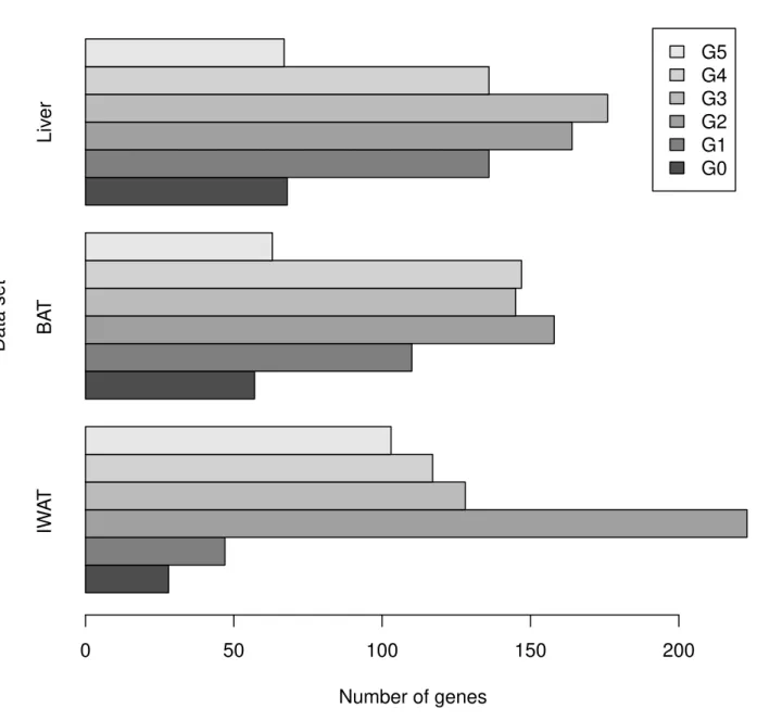
The Results of phase classification are summarized inTable 1andFig 5. In the IWAT data, and with a confidence levels of at least 95%, 28 genes peak at PhaseG0, 47 at PhaseG1, 223 at

PhaseG2, 128 at PhaseG3, 117 at PhaseG4, and 103 at PhaseG5, representing 4.33%, 7.27%,

34.52%, 19.81%, 18.11%, and 15.94% of the oscillating genes, respectively. In the BAT data, 57 peak at PhaseG0, 110 at PhaseG1, 158 at PhaseG2, 145 at PhaseG3, 147 at PhaseG4, and 63 at

Table 1. Number of genes in each phase for the IWAT, BAT and Liver data sets.

Phase/Data IWAT BAT Liver

PhaseG0 28 57 68

PhaseG1 47 110 136

PhaseG2 223 158 164

PhaseG3 128 145 176

PhaseG4 117 147 136

PhaseG5 103 63 67

Total 646 680 747

(10)

PhaseG5, representing 8.38%, 16.17%, 23.23%, 21.32%, 21.61%, and 9.26% of the oscillating

genes, respectively. For the Liver data set, 68 genes peak at PhaseG0, 136 at PhaseG1, 164 at

PhaseG2, 176 at PhaseG3, 136 at PhaseG4, and 67 at PhaseG5, representing 9.10%, 18.20%,

21.95%, 23.56%, 18.20%, and 8.97% of the oscillating genes, respectively. The method for esti-mation of phase assignment confidence that we proposed allows some useful observation even on the testing data. For instance, we may ask how uniform is gene expression over time? For

IW

A

T

BA

T

Liv

er

G5

G4

G3

G2

G1

G0

Number of genes

Data set

0

50

100

150

200

Fig 5. Barplot of the number of genes against phases.Bar plot summarizing the number of genes in each phase for the IWAT, BAT and Liver data sets from the results inTable 1.

(11)

the experiments collecting data in circadian timeline we can formulate the Null-hypothesis stating that the same number of genes can be confidently assigned to each phase group. The alternative hypothesis would state that at least one phase group has significantly different num-ber of genes. Both hypotheses are consistent with the overall numnum-ber of rhythmically expressed genes and cannot be testes without quantitative estimation of confidence of phase assignment. In our test data we apply the samep= 0.05 threshold, but observe fewer genes peaking at one of the phases. In biological terms this means the in murine adipose tissue there is a period (morning hours) when the overall gene expression activity is lower compared to all other times of the day.

However, it is even more important that our method can be applied to increase precision of observation in many studies involving timeline observation of gene expression. The sampling fre-quency still imposes limitation on our ability to separate molecular events (such as peak of gene expression) in time. To know the time of peak expression more precisely the experiment has to be repeated with higher a number of time points (for example, one sample every 2 hours rather than every 4 hours). However, with our method we can refine the existing data. For the groups peaking at a certain time we can be confident (at a selected confidence level) that certain genes peak at a certain time and filter out genes peaking sometime between out observation time points. This confidence is essential for functional annotation of co-expressed genes and can be critical in analysis of permutation of gene activity in reaction to environment or medication.

Strengths and boundaries

We compare the proposed method with some competing algorithms, namely Fisher’sg-test [16], Permutation test [15], and JTK-CYCLE [17]. All methods except the permutation test are implemented in R, and run on an Itel corei7 at 3.40 GHz. The permutation test is implemented in C++. Tables2,3and4show some results for the IWAT, BAT and Liver data sets.

In this paper, we are interested in genes that may have a peak expression coinciding or near one of the observation points. We approximate their expression profiles by an ideal cosine wave of the form:

C

φðtÞ ¼ cos 2p

T t φ

;t¼0;4;8; :::;44;φ2 ½0;2p½: ð9Þ

We know that for circadian genes we haveT= 24h. For the data sets used in this paper, the measurements time aret2{0,4,8,. . ., 44}. Since we are interested by theﬁrst peak expression time, the possible time points to be considered aret2{0,4,8,. . ., 20}. If we solve for equations C_φ₍_t_{) = 0 for}_t₂_{0,4,8,. . ., 20}, we obtainφ2{0,π/3, 2π/3,π, 4π/3, 5π/3}, this explains the use ofπ/3 as a resolution power of estimated phase inEq (2). If we choose different values of the resolution power of estimated phase, the peak time of the generated ideal cosine waves will not necessarily coincide with one of the time points when the measurements were taken. Neverthe-less, the method is general. It can work for periods other than 24 hours, for different spacing time points, and it can works with a larger number of cosines waves with smaller phases. For example, for any integerkwe can generate 2kcosine waves using the equation:

C

i¼cos 2p

1 24t

1 2ki

¼cos p 1 12t

1

ki

;t¼0;4;8; :::;44;i¼0;1;2; :::;2k 1: ð10Þ

(12)

that the average CPU timings increases with number of generated cosine waves and the num-ber of bootstrap replications.

Table 3shows some timing results for the three different datasets; Fisher’sg-test is faster, followed by JTK-CYCLE and then the proposed method (one replication). We note here that the computing performance of the proposed method can be enhanced considerably (See

Remark 4).

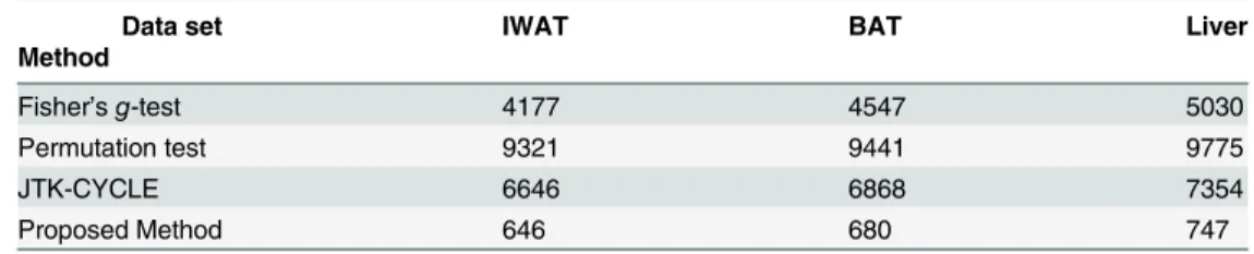
Table 4shows the number of identified circadian genes. The Permutation test identifies the highest number, followed by the JTK-CYCLE and then Fisher’sg-test. Our method is not developed for detecting all the circadian genes, but rather it detects, with high confidence, the circadian gene for which the peak time (the phase) is near one of the time points; estimates this phase, and constructs a confidence interval for it. This explains the small number of circadian genes detected by our method compared to the competitors.

Remark 2. This experiment design is rather typical for circadian biology. Some experiments collect samples at different intervals, such as 3h or, rarely, every 2h. Higher sampling frequency improves resolution ability, but costs a lot more and is harder to implement.

Remark 3. Gene expression profiles are analyzed independently, thus it is possible that a researcher may find few or none of the gene confidently peaking at a given time. In fact, in the data set on which we tested the method, gene expression has a quiet period at which relatively few genes are active.

cosine waves with smaller phases generated using theEq (10).The number of bootstrap replicationsRis in {9, 99, 999}.

Data set IWAT BAT Liver

Method R= 9 R= 99 R= 999 R= 9 R= 99 R= 999 R= 9 R= 99 R= 999

Proposed Method usingEq (2) 3.71(m) 32.20(m) 5.53(h) 3.67(m) 32.54(m) 5.75(h) 3.61(m) 32.39(m) 5.79(h) Proposed Method usingEq (10) 11.40(m) 1.86(h) 19.83(h) 11.39(m) 1.82(h) 19.83(h) 11.45(m) 1.81(h) 19.73(h) doi:10.1371/journal.pone.0131111.t002

Table 3. IWAT, BAT and Liver data sets: timings (seconds) for Fisher’sg-test, Permutation test, JTK-CYCLE, and the proposed method on one bootstrap replication.

Method

Fisher’sg-test 11.79(secs) 12.27(secs) 11.87(secs)

JTK-CYCLE 16.49(secs) 14.34(secs) 14.59(secs)

Proposed Method (One replication) 22.50(secs) 22.63(secs) 22.41(secs) doi:10.1371/journal.pone.0131111.t003

Table 4. IWAT, BAT and Liver data sets: number of circadian genes identified using Fisher_’sg-test, Permutation test and JTK-CYCLE respectively.

Method

Fisher’sg-test 4177 4547 5030

Permutation test 9321 9441 9775

JTK-CYCLE 6646 6868 7354

Proposed Method 646 680 747

(13)

Remark 4. We note that the computational performance of the proposed method can be enhanced. In fact, if we avoid usingloopsin R script that process one element per iteration, and instead we useapplyfamily of functions that process whole rows, columns, or lists, the comput-ing time is reduced significantly. In this case we need just 0.001 second to run the method for one replication usingEq (2), and we need 0.008 second to run the method using higher number of cosine waves usingEq (10).

Supporting Information

S1 R Codes. R Analysis Codes.

(PDF)

S1 Data. IWAT data measurements.

(TXT)

S2 Data. BAT data measurements.

(TXT)

S3 Data. Liver data measurements.

(TXT)

Acknowledgments

We thank Christopher Leonard from QScience, Qatar Foundation, for improving the quality of the manuscript.

Author Contributions

Analyzed the data: ME. Wrote the paper: ME AP. Developed the algorithm and implemented the code: ME. Discussed the results: AF AP. Formulated the problem: AP.

References

1. Zhang R, Lahens NF, Ballance HI, Hughes ME, Hogenesch JB. A circadian gene expression atlas in mammals: implications for biology and medicine. Proceedings of the National Academy of Sciences. 2014; 111(45):16219–16224. doi:10.1073/pnas.1408886111

2. Klevecz RR, Li CM, Marcus I, Frankel PH. Collective behavior in gene regulation: the cell is an oscilla-tor, the cell cycle a developmental process. FEBS journal. 2008; 275(10):2372–2384. doi:10.1111/j. 1742-4658.2008.06399.xPMID:18410382

3. Ptitsyn AA, Reyes-Solis G, Saavedra-Rodriguez K, Betz J, Suchman EL, Carlson JO, et al. Rhythms and synchronization patterns in gene expression in the Aedes aegypti mosquito. BMC genomics. 2011; 12(1):153. doi:10.1186/1471-2164-12-153PMID:21414217

4. Panda S, Antoch MP, Miller BH, Su AI, Schook AB, Straume M, et al. Coordinated transcription of key pathways in the mouse by the circadian clock. Cell. 2002; 109(3):307–320. doi:10.1016/S0092-8674 (02)00722-5PMID:12015981

5. Storch KF, Lipan O, Leykin I, Viswanathan N, Davis FC, Wong WH, et al. Extensive and divergent circa-dian gene expression in liver and heart. Nature. 2002; 417(6884):78–83. doi:10.1038/nature744PMID: 11967526

6. Bray MS, Shaw CA, Moore MW, Garcia RA, Zanquetta MM, Durgan DJ, et al. Disruption of the circa-dian clock within the cardiomyocyte influences myocardial contractile function, metabolism, and gene expression. American Journal of Physiology-Heart and Circulatory Physiology. 2008; 294(2):H1036–

H1047. doi:10.1152/ajpheart.01291.2007PMID:18156197

7. Ptitsyn AA, Gimble JM. True or false: All genes are rhythmic. Annals of medicine. 2011; 43(1):1–12. doi:10.3109/07853890.2010.538078PMID:21142579

(14)

Journal of Statistical Software. 2009; 29(5):1–19.

10. Davison AC, Hinkley DV. Bootstrap methods and their application. vol. 1. Cambridge university press; 1997.

11. Efron B. Bootstrap methods: another look at the jackknife. The annals of Statistics. 1979;p. 1–26.

12. Efron B, Efron B. The jackknife, the bootstrap and other resampling plans. vol. 38. SIAM; 1982.

13. Hall P. On the bootstrap and confidence intervals. The Annals of Statistics. 1986;p. 1431–1452.

14. Zvonic S, Ptitsyn AA, Conrad SA, Scott LK, Floyd ZE, Kilroy G, et al. Characterization of peripheral cir-cadian clocks in adipose tissues. Diabetes. 2006; 55(4):962–970. doi:10.2337/diabetes.55.04.06. db05-0873PMID:16567517

15. Ptitsyn AA, Zvonic S, Conrad SA, Scott LK, Mynatt RL, Gimble JM. Circadian clocks are resounding in peripheral tissues. PLoS Comput Biol. 2006; 2(3):e16. doi:10.1371/journal.pcbi.0020016PMID: 16532060

16. Wichert S, Fokianos K, Strimmer K. Identifying periodically expressed transcripts in microarray time series data. Bioinformatics. 2004; 20(1):5–20. doi:10.1093/bioinformatics/btg364PMID:14693803 17. Hughes ME, Hogenesch JB, Kornacker K. JTK CYCLE: an efficient nonparametric algorithm for

detect-ing rhythmic components in genome-scale data sets. Journal of biological rhythms. 2010; 25(5):372–