Simulation of Triple Junction Motion
with Arbitrary Surface Tensions
Nur Shofianah, Rhudaina Z. Mohammad, Karel Svadlenka
Abstract—We simulate triple junction motion that is given by the gradient flow of surface energy with arbitrary sur-face tensions of the individual intersur-faces. The foundation of the method is the diffusion-based BMO algorithm in vector-valued formulation. We modify the original vector-vector-valued BMO method so that it can accommodate motions for any triple of surface tensions leading to the possibility of a nonsymmetric junction. The main idea of the modification is to adjust both the reference vectors and the coefficients in the underlying diffusion system. Moreover, we improve the method by using vector-valued projection triangle and also address the volume-preserving problem. Analysis and numerical results of this generalized vector-valued BMO algorithm are presented.
Index Terms—triple junction motion, mean curvature flow, surface tension, vector-valued thresholding
I. INTRODUCTION
T
HE problem of simulating the motion of interfaces with triple junction according to some curvature-dependent speed arises in many applications, e.g., grain growth [1], image processing [2], multiphase flow [3]. Equal surface ten-sions lead to symmetric triple junction, which is well-known as the symmetric Herring condition (interfaces meeting at120◦). On the other hand, arbitrary surface tensions lead to
nonsymmetric triple junctions.
To treat such motions, several methods have been devel-oped. Bronsard et. al [11] uses the reaction-diffusion equation
ut=ε∆u−
1
ε∇uW(u), (1)
to model triple junctions. Here,ε >0 is a small parameter andW is a well potential, a non-negative function which has three minima for the three-phase case. This so-called phase-field method represents the phase boundary as an interfacial layer. In [11] the authors showed that the interfaces in the solution of (1) move with a velocity proportional to the curvature of the interface and in its sharp interface limit
(ε→0), one obtains the Young’s law at the junction. How-ever, this method has difficulties in the numerical solution when ε < ∆x, where ∆x is the spacing grid. The only remedy is to take ∆εx ≪ 1, which is impractical numer-ically [4]. Moreover, it is also necessary to appropriately determine parameters of the well-potential function which Manuscript received December 31, 2013; revised June 27, 2014. The work of the first author is supported by the Directorate General of Higher Education (DIKTI), Ministry of National Education, Indonesia and the second author by the Japanese Government (Monbukagakusho: MEXT) Scholarship Grant. This work was also supported by JSPS A3 Foresight Program ”Computational Applied Mathematics 2014-2019”.
Nur Shofianah and Rhudaina Z. Mohammad are with the Graduate School of Natural Science and Technology, Kanazawa University, 920-1192 Japan, e-mail: nur [email protected], [email protected]
Karel Svadlenka is with Institute of Science and Engineering, Kanazawa University, 920-1192 Japan, and Institute of Mathematics, Academy of Sciences of the Czech Republic, Prague, Czech Republic, e-mail: [email protected]
amounts to a complicated minimization problem. Garcke et al. [12] performed numerical simulations for a multiphase field model and showed that for suitably chosen parameters (which they determined based on numerical experiments), numerical results agree with the formal asymptotic expansion of [13] and yield the correct motion.
On the other hand, Zhao et al. [17] developed a numerical algorithm capturing the interfaces based on the level set method of Osher et al. [18]. This method is able to deal with topological singularities and nonsmooth data. Moreover, it can be extended to the multiphase setting by introducing as many level set functions as there are phases and imposing an additional constraint on the constrained flow problem so that the level sets do not overlap or create vacuums. However, such a constraint has an unwanted influence on the motion and the volume of phases is not sufficiently controlled by the method.
Merriman, Bence and Osher [4] introduced the BMO method, an implicit scheme for realizing interfacial motion by mean curvature for symmetric junctions, which alternately diffuses and sharpens characteristic function for each phase region. For two-phase case, it has been shown that the method converges to motion by mean curvature [5], [6], [7]. Ruuth [8] generalized the BMO method to nonsymmetric triple junctions by replacing the thresholding step with a new decision, i.e., by using a projection triangle. This generalized method also allows for normal velocity equal to a positive multiple of the curvature of the interface plus the difference in bulk energies for prescribed junction angles. Svadlenka et al. [3] reformulated the BMO algorithm in vector-valued formulation for multiphase motion. This vector-valued for-mulation is essential for implementing constraints and for dealing with more general motions. However, it is restricted to the symmetric case. Mohammad et al. [9], [10] improved the symmetric multiphase BMO algorithm of [3] by intro-ducing a signed distance vector-valued function.
In this work, we consider three evolving curves meeting at a junction and having arbitrary surface tensions. We achieve the simulation of such a triple junction by generalizing the two main ingredients of the method in [3]: the reference vec-tors (corresponding to the positions of wells in the phase-field method) and the way of diffusing. Moreover, we improve the scheme by including a modification of the projection step in [8]. The developed method is applicable to constrained motions.
velocity and find the suitable modification for the coeffi-cients of underlying diffusion system. Section VI presents a correction by projection triangle. Numerical method and its implementation are explained in Section VII. Finally, Section VIII shows several numerical tests.
II. EQUATIONS OFTRIPLEJUNCTION
In this section, we write the total surface energy of the curves and compute its first variation to get the normal velocity for each interface and the condition that has to be satisfied at triple junction.
We consider three evolving curvesγi(s),s∈[pi, qi], i=
1,2,3, which lie inside a fixed smooth regionΩofR2, meet the outer boundary ∂Ω at a right angle and get together at a triple junction xT = γi(qi), i = 1,2,3. Each curve has different surface tensionσi.
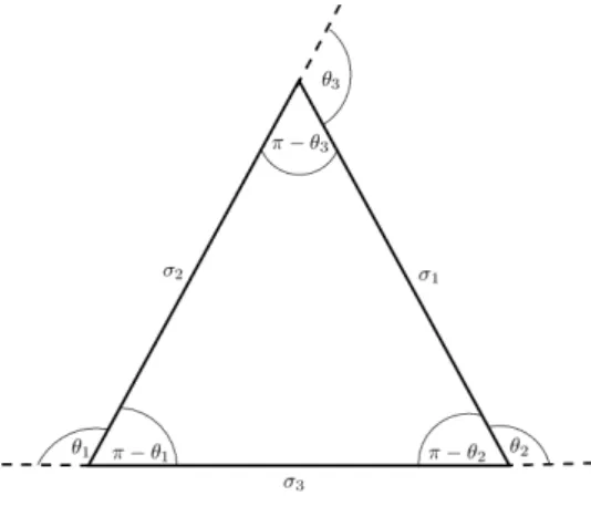
Fig. 1. Triple Junction
Then the surface energy of all curves is given by
L(γ) = 3
X
i=1
Z
γi
σidl=
3
X
i=1
Z qi pi
σi |γi′(s)|ds.
The gradient flow of surface energy [19] can be found from its variation. Define the tangential vectorti, curvatureκiand outer normal ni of curveγi by
ti=
γ′
i
|γ′
i|
, κi=−
γ′
ixγiy′′ −γiy′ γix′′
|γ′
i|3
, ni=
1
|γ′
i|
(γiy′ ,−γix′ ).
Then for a smooth vector fieldϕvanishing near the boundary
∂Ω,
d
dǫL(γ+ǫϕ(γ))|ǫ=0=
3
X
i=1
Z qi pi
σiti·
d
ds(ϕ(γi)) ds
= 3
X
i=1
−
Z
γi
(σiκini)·ϕdl+σiti·ϕ(xT)
.
From this result, the motion by gradient flow satisfies 1) The normal velocity of interface
vi=σiκi. (2)
2) Condition at triple junction
3
X
i=1
σiti= 0. (3)
The junction condition (3) is the balance of forces which is well-known to be equivalent to the Young’s law
sinθ1
σ1
=sinθ2
σ2
=sinθ3
σ3
,
whereθ1, θ2, θ3 are the angles at the junction (see Figure 1).
Fig. 2. Relating surface tensions to junction angles.
Noting the connection of the above formula to the triangle in Figure 2 and using the law of cosines, we obtain the junction angles as [14]:
cos(π−θ1) =
σ2 3+σ
2 2−σ
2 1 2σ2σ3
,
cos(π−θ2) =
σ2 1+σ
2 3−σ
2 2 2σ1σ3
, (4)
andθ1+θ2+θ3= 2π.
Note that we can compute the stable angles with any given triple of surface tensions, as long as the triple satisfies the triangle inequality.
III. VECTOR-VALUEDBMO
The basis of our method is the vector-valued BMO algo-rithm [3]:
1) Define reference vectors pi of dimension two, each corresponding to a phase Pi fori= 1,2,3.
2) Given a partition Pi, i = 1,2,3, set u0(x) = pi for
x∈Pi. 3) Repeat
• Solve the vector-valued heat equation with initial
condition u0:
ut(t, x) = ∆u(t, x) for (t, x)∈(0,∆t]×Ω,
∂u
∂n(t, x) = 0 on (0,∆t]×∂Ω.
• Update u0 by identifying the reference vector
which is closest to the solution u(∆t, x): u0(x) =pj,
This redistribution of reference vectors determines the configuration of each phase after time∆t.
The paper [3] deals only with symmetric junctions and therefore, the above algorithm works with symmetric refer-ence vectors and simple heat equation in the diffusion step, as is formally proved there. However, for arbitrary junction angles, this setting is not sufficient and has to be generalized. We will do so in the following two sections.
IV. JUNCTIONSTABILITY
We consider three straight lines meeting at the origin with the given stable angles as in Figure 3. The fact that this configuration is stable will yield a condition on the selection of reference vectors for the BMO algorithm.
Fig. 3. Configuration of a stable junction.
The triple junction does not move ifu(t,0,0) =0 for all
t > 0, where u is the solution of the heat equation. This means
1 4πt
3
X
i=1
pi
Z
R2∩P
i
exp(−|x|
2
4t ) dx=0.
Since by radial symmetry we can compute the integral of the wedgePi as
Z
Pi
e−|x|2
dx=θi 2,
we get
θ1p1+θ2p2+θ3p3=0. (5)
The above relation is a one-dimension higher BMO ana-logue of Young’s law (3) in the sense that the reference vectorspi are distributed in the whole phase regionsPi and, thus, the equilibrium condition is related to area integrals, which results in weights equal to junction angles.
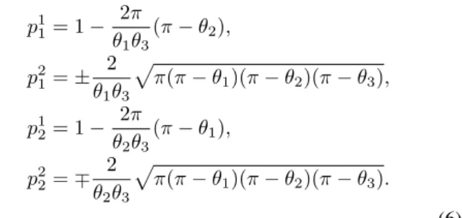
The vector equation (5) and the condition obtained in the next section that the lengths of pi, i = 1,2,3, must be equal, form a systems of equations for the components ofpi. Since the reference vectors are determined up to rotation and scaling, we can choose one reference vector arbitrarily, e.g., we set p3 = (1,0). This closes the system and its solution
can be written as
p11= 1− 2π θ1θ3
(π−θ2),
p2 1=±
2
θ1θ3
p
π(π−θ1)(π−θ2)(π−θ3),
p1 2= 1−
2π θ2θ3
(π−θ1),
p22=∓ 2
θ2θ3
p
π(π−θ1)(π−θ2)(π−θ3).
(6) The possible choices for the sign of the second component follow from the invariance of the reference vectors with respect to flipping.
V. INTERFACEVELOCITY
Here we study the modification of the original BMO algorithm yielding the correct interface velocitiesvi=σiκi. The idea is to consider, instead of the heat equation, the general diffusion system
u1
t+du
2
t =a∆u
1+b∆u2,
du1
t+eu
2
t=b∆u
1
+c∆u2
, u1
u2
!
(t= 0) = u 1 0
u2 0
!
,
(7)
and determine its coefficientsa, b, c, d, e, so that we obtain the desired interface velocities. We will show that this leads to a system of nonlinear equations fora, b, c, d, e. Moreover, we check that the change of the underlying diffusion system does not influence the arguments of the previous section on junction stability.
Note that we restrict our considerations to symmetric coefficient matrices. This is due to the fact that in order to incorporate phase-volume preservation, we use the varia-tional structure of the system in an essential way (see Section VII.B).
The system (7) can be rewritten in the form
˜
ut=A∆˜u,
where
˜
u=
˜
u1 ˜
u2
=
1 d
d e
u1
u2
,
and
A= 1
e−d2
ae−bd b−ad be−cd c−bd
.
We assume thatA is positive definite and diagonalize it in the following form
A=KΛK−1
with Λ =
λ1 0
0 λ2
.
The eigenvalues ofAare given by
λ1,2=
ae+c−2bd±r
2(e−d2) ,
wherer=p
(ae−c)2+ 4(ad−b)(cd−be).
Hence, we get the matrixK consisting of eigenvectors as
K= 1
2r
ae−c+r 2(ad−b) 2(be−cd) ae−c+r
The original problem is transformed into w1
t =λ1∆w1,
w2
t =λ2∆w2,
w1
w2
!
(t= 0) = w 1 0
w2 0
!
=M u
1 0 u2 0 ! , (8) where w1 w2 =M u1 u2
,withM =K−1
1 d
d e
.
The solution to the transformed problem (8) in the whole R2
is
wi(t, x) = 1
4πλit
Z
R2
wi
0(ξ)e−
|x−ξ|2
4λit dξ, i= 1,2, (9)
where
wi
0|Pj = ((Mu0)|Pj)
i= (Mp
j)i, i= 1,2, j= 1,2,3.
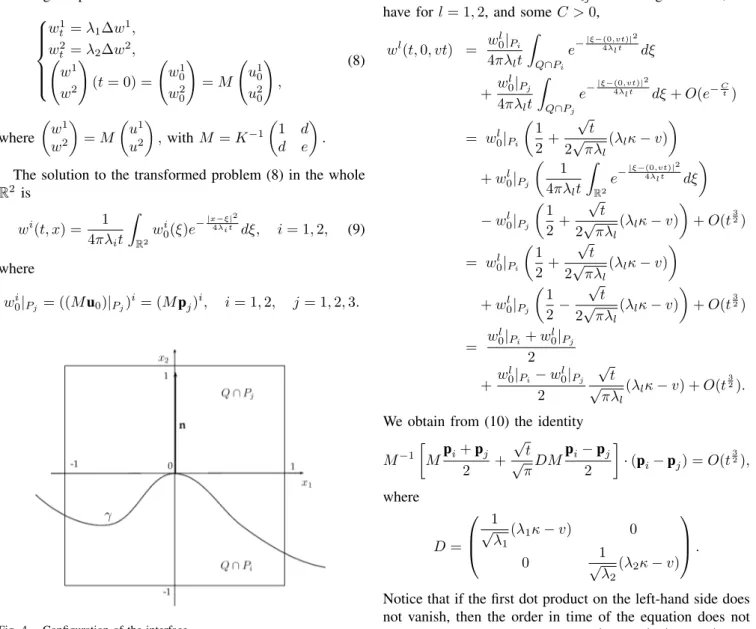
Fig. 4. Configuration of the interface.
Now, let us calculate the velocity of the interface for the above diffusion system. We consider a point on the interface
γ=∂Pij between phasePi andPj. We translate and rotate the coordinate system so that the chosen point lies in the origin and the outer normal at the point agrees with the positivex2-direction. We defineQ= [−1,1]×[−1,1]. Then
the normal velocity v of the interface is found from the relation, expressing the condition on the interface position along thex2-axis after time t, i.e.,
u(t,0, vt)·(pi−pj) = 0. (10) We can write the solution of the transformed problem (8) as
w(t,0, vt) =
1 4πλ1t
R
R2w 1 0(ξ)e−
|ξ−(0,vt)|2
4λ1t dξ
1 4πλ2t
R
R2w 2 0(ξ)e−
|ξ−(0,vt)|2
4λ2t dξ
.
By the techniques in [5] and [15], we get
1 4πλ1t
Z
Q∩Pi
e−|ξ−(0,vt)|
2 4λ1t dξ= 1
2+
√ t
2√πλ1
(λ1κ−v)+O(t 3 2),
(11)
where κis the curvature of ∂Pij at the origin. Hence, we have forl= 1,2, and someC >0,
wl(t,0, vt) = w0l|Pi
4πλlt
Z
Q∩Pi
e−|ξ−(0,vt)|
2 4λlt dξ
+w
l
0|Pj
4πλlt
Z
Q∩Pj
e−|ξ−(0,vt)|
2
4λlt dξ+O(e−Ct)
= w0l|Pi
1 2 +
√ t
2√πλl
(λlκ−v)
+wl
0|Pj
1 4πλlt
Z
R2
e−|ξ−(0,vt)|
2 4λlt dξ
−wl
0|Pj
1 2 +
√ t
2√πλl
(λlκ−v)
+O(t32)
= wl
0|Pi
1
2 +
√ t
2√πλl
(λlκ−v)
+wl
0|Pj
1
2 −
√ t
2√πλl
(λlκ−v)
+O(t32)
= w
l
0|Pi+w l
0|Pj
2
+w
l
0|Pi−w l
0|Pj
2
√ t √
πλl
(λlκ−v) +O(t
3 2).
We obtain from (10) the identity
M−1
Mpi+pj
2 +
√ t √
πDM
pi−pj
2
·(pi−pj) =O(t32),
where D= 1 √ λ1
(λ1κ−v) 0
0 √1
λ2
(λ2κ−v)
.
Notice that if the first dot product on the left-hand side does not vanish, then the order in time of the equation does not match. This leads to the condition(pi+pj)·(pi−pj) = 0, meaning that the lengths of reference vectors have to be equal (see Section IV). Then we obtain
(pi−pj)TM−1
DM(pi−pj) =O(t),
which is, up to orderO(t), equivalent to
µ1
p
λ1κ− 1
√ λ1
v
+µ2
p
λ2κ− 1
√ λ2
v
= 0,
where
µ1= m11m22(p 1
ij)
2
−m12m21(p 2
ij)
2
+ (m12m22−m11m21)p 1
ijp
2
ij,
µ2= −m12m21(p 1
ij)
2
+m11m22(p 2
ij)
2
−(m12m22−m11m21)p1ijp2ij,
with pij = pi −pj and m11, m12, m21, m22 denote the
entries of the matrix M. Finally, we get the velocity of interfaceγk (k6=i, j)in the form
vk=
µ1
√ λ1+µ2
√ λ2
µ2
√ λ1+µ1
√ λ2
p
λ1λ2κk.
velocities. Hence, it is reasonable to try to setd= 0, e= 1, so that our diffusion system becomes
ut=A∆u, (12)
with A =
a b
b c
. We could have done so from the beginning of this section but, as we will see below, the resulting nonlinear system for a, b, c is hard to analyze theoretically, which led us to keep the parameters d and e
as a last resort in case the three-parameter system cannot be solved. In this case, we get the interface velocities
vk=
µ1(a+c+r) + 2µ2
√ ac−b2
µ2(a+c+r) + 2µ1
√ ac−b2
p
ac−b2κ
k, (13) wherer=p
(a−c)2+ 4b2 and
µ1= [(a−c+r)(p1i −p1j) + 2b(p2i −p2j)]2,
µ2= [2b(p1i −p1j)−(a−c+r)(p2i −p2j)]2.
From (13) and (2), we have a nonlinear system consisting of three equations for the coefficients a, b and c, which is solved numerically. First, we simplify it by setting
x = α+
p
β2+ 1
p
α2−β2−1,
y = β+pβ2+ 1,
z = bpα2
−β2
−1,
where α = (a+c)/(2b) and β = (a−c)/(2b). Then the above system in terms ofx, y, z becomes
(p1
ijy+p
2
ij)
2
x+ (p1
ij−p
2
ijy)
2
(p1
ij−p
2
ijy)
2x+ (p1
ijy+p
2
ij)
2z=σk
for (i, j, k) = (2,3,1),(1,3,2),(1,2,3). We take any two equations from this system and solve for x, z analyti-cally, which is possible, since the corresponding equation is quadratic. Due to this fact we get two different solutions for
x, z. For each such pair of x, z we use a numerical method (such as Newton’s method) to find the rootyof the remaining equation. There may exist several roots fory. For each such combination of x, y, zwe recover α, βandb by
α=(x 2
+ 1)(y2 + 1) 2(x2−1)y , β =
y2
−1
2y , b=± x(y2
+ 1) (x2−1)y.
The coefficients a and c are then obtained easily. The number of cases doubles because of two possible signs for
b. All triples(a, b, c)obtained in the described way are then checked if they solve the system and the appropriate triple is selected.
Since the nonlinear system is very complicated, we were not able to prove the unique existence of solution using analytical methods such as fixed point theory. However, in using the above method we can always find a solution, except when b= 0, which occurs when two of the surface tensions are equal. In that case, the system simplifies in such a way that it can be solved fully analytically.
Remark. For the initial condition in Figure 3, at the triple junction we have
wi(t,0) = 1
4πλit
Z
P1 +
Z
P2 +
Z
P3
wi
0(ξ)e−
|ξ|2
4λitdξ
= 1
π
θ
1
2w
i
0|P1+
θ2 2 w
i
0|P2+
θ3 2w
i
0|P3
.
Therefore,
w(t,0) = 1
2πM(θ1p1+θ2p2+θ3p3).
For junction stability, we requireu(t,0) =M−1
w(t,0) =0. This condition is equivalent to
θ1p1+θ2p2+θ3p3=0,
which is in agreement with (5).
This result shows that no matter how we change the diffusion equation, the stability condition (5) will not be affected. Hence, the selection of reference vectors can be done independently of the diffusion equation.
VI. CORRECTION BYPROJECTIONTRIANGLE In the previous sections, we have derived an extension of the vector-valued BMO algorithm to include the case of nonsymmetric junctions and general interface velocities. We have shown that, for a suitably selected diffusion system, if an interface point is sufficiently far from the junction, the interface velocity at that point will satisfy the desired formula
vi=σiκi, and that, for a suitably selected reference vectors, the junction will be stationary for the initial configuration of three straight lines meeting at the junction with stable contact angles.
However, the above analysis does not address the close vicinity of the triple junction. In fact, by formal calculations it can be made clear (see Appendix A) that the correct interface velocity is obtained only with an exponentially decreasing error with respect to the distance of the considered interface point to the junction. Indeed, numerical tests proved that the stable configuration consisting of three straight lines slightly curves in the neighborhood of the junction. This fact produces errors in the angles of the moving junction.
Therefore, we include a correction step based on the notion of a projection triangle given by Ruuth [8]. The idea is to first investigate how the stable configuration of three straight lines deforms, and use this information to project the phase regions back into the correct position in each step of the BMO algorithm. For details of the construction of the projection triangle we refer to [8].
The original method in [8] uses the scalar setting, i.e., it diffuses separately characteristic functions for each of the three phase regions of the stable configuration (Figure 3) which yields three values of diffused function at every point in the domain. These three values are positive and sum up to one, thus, taken as points inR3, lie inside a triangle on a hyperplane ofR3. The straight lines of the stable configura-tion are mapped on the triangle as dividing curves. In order to relate our vector-valued formulation to the construction in [8], for(i, j, k)∈ {(1,2,3),(2,3,1),(3,2,1)} we introduce the functions
fi(t, x) =
u(t, x)·(pj+pk)−1−pj·pk
(pi−pj)·(pj+pk) , (14)
Note that (14) is a generalization of the functionwi(t, x)in [3], Section 2.2.2, for general reference vectors (6). Since u(0, x) =pi forx∈Pi, one can easily check that
fi(0, x) =χi(x), i= 1,2,3,
However, the advantage of our vector-valued approach is that we do not have to perform separate diffusions and subsequently identity the hyperplanex1+x2+x3= 1. It is
sufficient to diffuse the vector-valued initial condition as in Figure 3 and record the images of the straight lines. In this way, we obtain a projection triangle that can be used directly for the functionu in the BMO algorithm.
We summarize the construction of the projection triangle in the generalized vector-valued formulation. Given an angle configurationθ1, θ2, θ3, we perform the following steps:
1) Define the lines (in polar coordinates)
ℓ12={(r, 1
2θ1) :r >0},
ℓ13={(r,− 1
2θ1) :r >0},
ℓ23={(r, 1
2θ1+θ2) :r >0},
and regionsP1, P2, P3, as in Figure 3.
2) Setu0(x) =pi forx∈Pi.
3) Apply the diffusion (7) to the initial condition u0 for
a timeτ ≤∆t, where ∆t is the BMO time step. 4) Map the values of the solution of step 3 along each line
ℓij onto the projection triangle to form the dividing linesℓ˜ij: ℓ˜ij={u(τ, x) :x∈ℓij}.
Fig. 5. Projection triangleT in vector-valued setting.
Notice that the values of the diffused functionufall inside the triangle T formed by the vectors p1,p2,p3 (Figure 5).
Moreover, because of (5), the dividing lines ℓ˜12,ℓ˜13,ℓ˜23
will always meet at the origin which corresponds to the circumcenter of T, and they approach the midpoints of edges of T on their other ends. This is in contrast to the projection triangles in [8], where the position of the junction shifts and the shape of dividing lines is distorted, especially for junction angles strongly deviating from the Herring symmetric case. This fact helps significantly to make the numerical computations stable, especially for the volume-preserving problem.
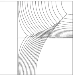
Figure 6 shows the resulting projection triangles for the
150◦−90◦−120◦junction and the135◦−90◦−135◦junction.
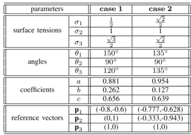
Since these two cases will be used in numerical tests, we list the coresponding parameters in Table I. As it sometimes happens in the numerical computations that the values of the functionu fall out of the projection triangle, we extend the dividing curves by straight lines connecting the junction to the midpoints of the edges.
(a) (b)
Fig. 6. Projection triangle for (a)150◦−90◦−120◦ and (b)135◦−
90◦−135◦triple junctions.
TABLE I
NUMERICAL PARAMETERS FOR CASE1AND CASE2
parameters case 1 case 2
surface tensions
σ1 12
√
2 2
σ2 1 1
σ3
√
3 2
√
2 2
angles
θ1 150◦ 135◦
θ2 90◦ 90◦
θ3 120◦ 135◦
coefficients
a 0.881 0.954
b 0.262 0.127
c 0.656 0.639
reference vectors
p1 (-0.8,-0.6) (-0.777,-0.628)
p2 (0,1) (-0.333,-0.943)
p3 (1,0) (1,0)
Remark. There is a close relation between the BMO algorithm and a splitting method for the phase-field equation (1), which repeats the following steps:
1) Diffuse for a time∆t
ut=ε∆u,
with initial condition u(0, x) =u0.
2) Solve
ut=−
1
εW
′(u), (15)
with initial condition u(∆t, x).
One can see that (15) corresponds to the thresholding step in BMO in the sense that the solution asymptotically separates into three regions with values equal to the minima of W. The dividing lines between these regions are the separatrices for the well potentialW. The well potential can be chosen as in [12] but, as mentioned in the Introduction, it is not easy to calibrate its parameters since they are not given by an explicit formula.
VII. THEALGORITHM
In this section, we summarize the above deliberations into a generalized vector-valued BMO scheme. First we present the basic version of the BMO algorithm and then comment on the method of incorporating the volume constraint.
A. Generalized vector-valued BMO algorithm
The generalized vector-valued BMO for three-phases mo-tion is as follows:
1) For given surface tensions, calculate junction anglesθi by (4).
3) Find the solutiona, b, cof (13) and setA=
a b
b c
.
4) Construct projection triangle according to the algo-rithm in Section VI.
5) For a given three phase initial configurationP1, P2, P3,
set
u0(x) =pi, x∈Pi.
6) Repeat until desired time
• Solve the diffusion system
ut=A∆u for(t, x)∈(0,∆t]×Ω, (16)
∂u
∂n = 0 on(0,∆t]×Ω, u(0, x) =u0(x) inΩ.
• Threshold according to the projection triangle
de-fined in step 4, i.e.,
u0(x) =pi if u(x)∈Ri, i= 1,2,3, whereRi are the regions in Figure 5.
The modified diffusion system is solved by using vector-type discrete Morse flow (DMF) [16], i.e., at each step we solve (16) by discretizing time ∆t =
h× N and successively minimizing the following functionals forn= 1, .., N overH1(Ω;R2)
:
Jn(u) =
Z
Ω
a
2|∇u 1
|2
+b∇u1
· ∇u2 +c
2|∇u 2
|2 dx
+
Z
Ω
|u−un−1|2 2h
dx. (17)
We approximate the functional (17) by using piecewise linear finite elements. The minimizers are found by steepest descent method.
B. BMO algorithm with volume-constraint
The minimization formulation of the vector-valued algo-rithm allows the inclusion of volume constraints via penal-ization. In particular, instead of the functionalJn in step 6, we minimize
Fn(u) =Jn(u) +
1
ǫ
3
X
i=1
|Vi−meas(Piu)|
2
.
Hereǫ >0is a small penalty parameter,Viis the prescribed volume of regionPiand the volumes corresponding touare obtained from the sets
Piu={x∈Ω;u(x)∈Ri}.
This means that we have to employ the projection triangle each time we evaluate the functional Fn.
VIII. NUMERICALRESULTS
We now present some numerical tests and examples of our method. All numerical experiments in this section are con-ducted on a[0,1]×[0,1]domain with time step∆t= 0.005
and DMF partition N = 30. Moreover, the phase interior angles at the triple junction are measured using the tangents to the quadratic interpolation of the piecewise linear interface in the neighborhood of the junction.
We begin by investigating the stability of the triple junction in terms of the angle measure and location of the junction.
Next, we look at the behavior of the triple junction motion for two cases (with and without axial symmetry). Finally, we present an example which incorporates the volume constraint and check the stability of the junction and preservation of the phase volumes of its stationary solution.
A. Junction Stability Test
Consider an initial condition where phase P2 consists
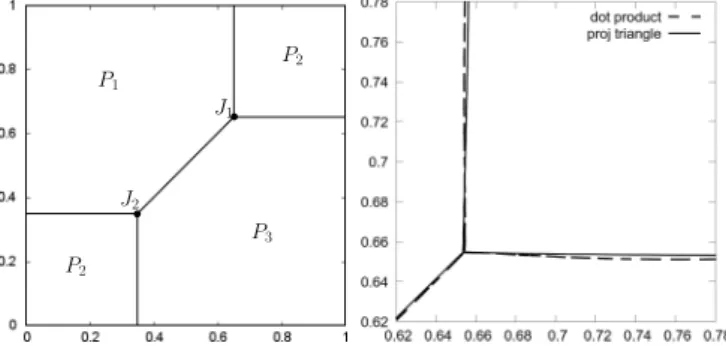
of two disjoint square regions on opposite corners of the domain; while the remaining regions above and below the liney=xare taken as phaseP1andP3, respectively (refer
to Figure 7a). In this setting, the interface network remains stationary for a135◦−90◦−135◦junction angle configuration.
We then, run our method under the case 2 setting (see Table I) and check the stability of the triple junction when the maximum dot product (without projection triangle) or projection triangle is used for phase detection. Here, the domain is triangulated into12,800elements (∆x= 0.0125).
P1
P3
P2
P2
b
J2
b
J1
Fig. 7. (a) Initial condition. (b) The stationary interface network around junctionJ1after time100∆tusing dot product and projection triangle for
phase detection.
The relative error of the stationary junction angle measures are summarized in Table II. We see that when the maximum dot product is used to locate the interface, the stationary interior angle in phaseP2 is of measure 90◦±5.11, while
the other two junction angles are approximately135◦±4.10;
thereby, yielding a relative error of at most 5.68%. On the other hand, utilizing the projection triangle in the phase detection scheme reduces the relative error to at most0.88%
with stationary junction angles of measure 90◦±0.78 and 135◦±1.19.
TABLE II
RELATIVEERROR INJUNCTIONANGLEMEASURES
phase maximum dot product projection triangle junctionJ1 junctionJ2 junctionJ1 junctionJ2 P1 −0.0083 −0.0081 0.0088 0.0077 P2 −0.0290 −0.0296 −0.0062 −0.0019 P3 0.0561 0.0568 −0.0039 −0.0087
In addition, both phase detection scheme shifted the junc-tion to a distance of at most 0.0065 for the dot product scheme and at most0.0057for the projection triangle. This can be accounted for by the approximation error in the con-struction of the projection triangle. Hence, our method stably preserves the angle conditions, in this case135◦−90◦−135◦.
B. Triple Junction Motion
In this section, we start with an initial condition where a T-shaped interface is rotated90◦counterclockwise where the
T-junction is at point (0.25,0.5). We take phase P2 as the
region to the left of linex= 0.25, and the remaining top and bottom regions as phases P1 andP3, respectively. We
trian-gulate the domain into 20,000 elements with ∆x = 0.01, and evolve the interface via our method using the projection triangle to determine the different phase regions at each time step. We then investigate the evolution of the triple junction in both cases.
1) Junction without Axial Symmetry: (Case 1 in Table I) Under the first case setup, we plot the evolution of the initial T-junction and its underlying interface network at different times in Figure 8.
Fig. 8. Evolution of the triple junction for case 1.
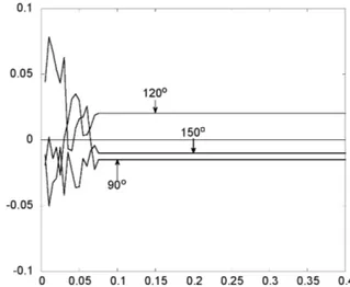
Fig. 9. Relative error of the junction angles at each time step.
Notice that for the first10time steps, the junction angles rapidly adjusts to approximate the 150◦−90◦−120◦ angle
conditions. Thereafter, the triple junction maintains phase interior angles of measure within 2.5% relative error (refer to Figure 9). Note that this approximation error in the stationary junction angles can be made smaller by increasing the precision in the construction of the projection triangle.
2) Axially Symmetric Junction: (Case 2 in Table I) We now look at the behavior of the junction motion when subjected to the second case. Note that since the surface
tensions on the 1−2 and2−3 interfaces are equal, that is,
σ1=σ3=√1
2, we expect these interfaces to symmetrically
evolve with respect to the horizontal line y = 0.5. This is in agreement with our numerical simulation shown in Figure 10.
Fig. 10. Evolution of the triple junction for case 2.
In the first 10 time steps, the triple junction rapidly approaches the135◦−90◦−135◦angle conditions. After which,
the interface gradually starts to move horizontally to the right. The transport velocity s of our numerical interface solution approaches 2√π
2, which is the exact velocity of
the constantly transported solution of the sharp interface problem, as shown in Figure 11.
Fig. 11. Transport velocities of the numerical interface solution at y= 0.45,0.47,0.49vs the constantly transported solution (sharp interf. sol.).
Moreover, we note that the shape of such a constantly transported profile in the axially symmetric case is deter-mined by:
v(y) =−σ1
s log(cos( s
σ1y)) +c,
Fig. 12. The shape of the numerical interface at timet= 30∆tvs the constantly transported solution.
C. Volume-preserving150◦−90◦−120◦ Double Bubble
Consider a three-phase volume-preserving case where two phases are identical squares with one common side of length
0.28. We take the outside region as phase P1, and the left
and right square regions as phase P2 and P3, respectively
(refer Figure 13).
We evolve this configuration via our method under case 1 setting in Table I. Moreover, we wish to preserve the volume of each phase region employing a penalization technique with parameter ǫ = 10−6
. Here, the domain is triangulated into
12,800elements with∆x= 0.0125. To locate the interface, we use a projection scheme determined by the maximum dot product. The numerical stationary interface solution is shown in Figure 13.
Fig. 13. (a) Initial Condition. (b) The stationary numerical solution in case 1.
To check the stability of the triple junction, we measure the junction angles at each time step and calculate the corresponding errors. We observe that the interior phase angles at the top and bottom triple junctions behave in the same manner, hence, we only plot the relative error in the measure of the top junction angle in Figure 14.
It is evident from the error plot that the triple junction first rapidly approximates the angle conditions, which is consistent with the previous results. Thereafter, the numerical solution gradually reaches a stationary state whose junction angles are of measure150◦±1.50,120◦±2.43, and90◦±1.36
yielding a relative error of at most 2%. This is consistent with the result in our stability test. Hence, one can achieve
Fig. 14. Relative error of the top junction angles at each time step.
a more precise result using the projection triangle to locate the interface.
TABLE III
PHASEVOLUMES UNDER PENALTY PARAMETERǫ= 10−6
.
phase prescribed vol stationary state vol absolute error P1 0.8432 0.84321 1.0×10⁻⁵ P2 0.0784 0.07840 3.0×10⁻⁶ P3 0.0784 0.07839 8.0×10⁻⁶
Moreover, it is clear from Table III that the phase vol-umes are preserved. Hence, the stationary numerical solution obtain using our method fairly approximates the volume-preserving solution of case 1.
IX. CONCLUSION
We have developed a method for numerical realization of triple junction motion with arbitrary surface tensions. Our method is based on the vector-valued BMO algorithm, which has been generalized and augmented by a correction step using projection triangle. Several numerical tests, including the volume-constrained motion, were performed.
APPENDIXA
FORMALANALYSIS OFNONSYMMETRICTRIPLE JUNCTION
We look at the formula for the solution of the system (7) with initial condition as in Figure 3 in more detail. From this, we will see that the interfaces close to the triple junction will not remain straight but will curve slightly.
Recalling the solution of the transformed problem (9), the solution of the original system is given by
u(t, x) =M−1
w=M−1
w1
w2
, (18)
wherew1, w2
are obtained from the formula
wi(t, x) =
3
X
j=1 (Mpj)i
Z
Pj
1 4πλit
e−|x−ξ|
2
4λit dξ, i= 1,2.
Set
erfc(s) = 1−erf(s) = √2 π
Z ∞
s
and
α(ϑ) =x1cosϑ+x2sinϑ,
β(ϑ) =x1sinϑ−x2cosϑ.
To see the specific form of the respective terms, we compute the integral
Z
P1
e−|x4−λtξ|2dξ
=
Z ∞
0
Z θ21 −θ1 2
e−(r−α(ϑ4))2 +λt β(ϑ)2rdϑdr
=
Z θ21 −θ1
2
e−β(4ϑλt)2
Z ∞
−√α(4ϑ)
λt
√
4λtz+α(ϑ)√4λte−z2dzdϑ
=√πλt
Z θ21
−θ1 2
α(ϑ)e−β4(ϑλt)2erfc
−√α(ϑ)
4λt
dϑ
+ 2λt
Z θ21 −θ1 2
e−β(ϑ)2 +4λtα(ϑ)2dϑ.
Rearranging the terms, we get
Z
P1
e−|x−ξ|
2 4λt dξ
= 2λt√π
Z
β(θ21)
√4
λt β(−θ1 2 )
√
4λt
e−z2erfc ±
r
|x|2 4λt −z
2
!
dz
+ 2λtθ1e−
|x|2
4λt.
Expressing the point x in polar coordinates as x = (scosϕ, ssinϕ), we get
1 2λt
Z
P1
e−|x−ξ|
2 4λt dξ
=√π
Z
ssin(θ21−ϕ)
√4
λt ssin(−θ1
2 −ϕ)
√
4λt
e−z2erfc ±
r
s2 4λt−z
2
!
dz
+θ1e−
s2
4λt, (19)
and similarly for the integrals over the regions P2 and P3.
From (19) we can conclude that: 1) If √s
t is close to zero, (19) approaches θ1 since the first term is negligible. Hence, from (18) we get the value of the solution
u(t, x)≈2θπ1p1+
θ2 2πp2+
θ3 2πp3,
which is in agreement with (5).
2) If the pointxis away from the triple junction and close to some of the interfaces, for instance the interface between phases P1 and P2, then the second term is
exponentially small. Moreover, ϕ ≈ θ1
2, and so the
first integral will be close toπ. Similarly, the integral over the regionP2 will be close to πand the integral
overP3 will be close to zero. Therefore, the solution
(18) at this pointxwill be
u(t, x)≈ 12(p1+p2),
which means that the interface will remain stationary as a straight line.
3) If the point xis in other position than the two cases mentioned above, the values of the above integrals will depend not only on xandt but also on the values of
λ1, λ2. As a consequence, the solutionu will depend
also on the coefficients a, b, c, and the corresponding interfaces may curve.
REFERENCES
[1] M. Elsey, S. Esodoglu, P. Smereka, “Diffusion generated motion for grain growth in two and three dimensions,” inJ. Comp. Physics, vol. 228, pp. 8015-8033, 2010.
[2] F. Catte, P. L. Lions, J. M. Morel, “Image selective smoothing and edge detection by nonlinear diffusion,” inSIAM J. Num. Anal., vol. 29, pp. 182-183, 1992.
[3] K. Svadlenka, E. Ginder, S. Omata, “A variational method for multi-phase volume-preserving interface motions,“ in Journal of Computa-tional and Applied Mathematics, vol. 257, pp. 157-179, 2014. [4] B. Merriman, J. Bence, S. Osher, “Motion of multiple junctions: a level
set approach,” inJ. Comp. Physics, vol. 112, pp. 334-363, 1994. [5] L. Evans, “Convergence of an algorithm for mean curvature motion,”
inIndiana Univ. Math. J., vol. 42, pp. 533-557, 1993.
[6] G. Barles, C. Georgelin, “A simple proof of convergence of an approx-imation scheme for computing motions by mean curvature,” inSIAM J. Numer. Anal., vol. 32, pp. 484-500, 1995.
[7] Y. Goto, K. Ishii, T. Ogawa, “Method of the distance function to the Bence-Merriman-Osher algorithm for motion by mean curvature,” in
Comm. Pure Appl. Anal., vol. 4, pp. 311-339, 2005.
[8] S. J. Ruuth, “A diffusion-generated approach to multiphase motion,” in
J. Comp. Physics, vol. 145, pp. 166-192, 1998.
[9] R. Z. Mohammad, K. Svadlenka, “Multiphase Volume-preserving Inter-face Motions via Localized Signed Distance Vector Scheme”, preprint. [10] R. Z. Mohammad, “Multiphase mean curvature flow: signed distance vector approach,” in Recent development in computational science: selected papers from the ISCS, vol. 4, pp. 115-123, 2013.
[11] L. Bronsard, F. Reitich, “On three-phase boundary motion and the singular limit of a vector-valued Ginzburg - Landau equation,” inArch. Ration. Mech. Anal., vol. 124, pp. 355-379, 1993.
[12] H. Garcke, B. Nestler, B. Stoth, “A multiphase field concept: numerical simulations of moving phase boundaries and multiple junctions,” in
SIAM J. Appl. Math, vol. 60, pp. 295-315, 1999.
[13] H. Garcke, B. Nestler, B. Stoth, “On anisotropic order parameter models for multi-phase systems and their sharp interface limits,” in
Physica D, vol. 115, pp. 87-108, 1998.
[14] X. Chen, J-S. Guo, “Self-similar solutions of a 2-D multiple-phase curvature flow,” inJ. Comp. Physics, D 229, pp. 22-34, 2007. [15] K. Ishii, “Mathematical analysis to an approximation scheme for mean
curvature flow, in: S. Omata, K. Svadlenka (Eds.), ISCS 2011,” in Math-ematical Sciences and Applications, vol. 34, GAKUTO International Series, pp. 67-85, 2011.
[16] E. Rothe, “Zweidimensionale parabolische Randwertaufgaben als Grenzfall eindimensionaler Randwertaufgaben,” inMath. Ann., vol. 102, pp. 650-670, 1930.
[17] H. Zhao, T. Chan, B. Merriman, S. Osher, “A variational level set approach to multiphase motion”, inJ. Comp. Physics, vol. 127, pp. 179-195, 1996.
[18] S. Osher, J. A. Sethian, “Fronts propagating with curvature dependent speed: Algorithms based on Hamilton-Jacobi formulations”, inJ. Comp. Physics, vol. 79, pp. 12-49, 1988.
[19] D. ˇSevˇcoviˇc and S. Yazaki, “On a gradient flow of plane curves minimizing the anisoperimetric ratio”, inIAENG International Journal of Applied Mathematics, vol. 43 (3), pp. 160-171, 2013.
Nur Shofianahwas born in Gresik, Indonesia, on November24th
, 1984. She received S.Si. degree and M.Si. degree in Mathematics from Sepuluh Nopember Institute of Technology, Surabaya, East Java, Indonesia, in 2007 and 2009, respectively.