CHANGE IN CONVERGENT EVOLUTION OF
NATURAL POPULATIONS
Identifying candidate genes
behind convergent evolution
in blind cave fish Astyanax
mexicanus
Martina Bradi
㾒
Dissertation presented to obtain the Ph.D degree in Biology
Instituto de Tecnologia Química e Biológica | Universidade Nova de LisboaOeiras,
1
CONVERGENT EVOLUTION OF NATURAL POPULATIONS
:
IDENTIFYING CANDIDATE GENES BEHIND CONVERGENT
EVOLUTION IN BLIND CAVEFISH
ASTYANAX MEXICANUS
0DUWLQD%UDGLü
Dissertation presented to obtain the Ph.D. degree in Biology at the
Instituto de Tecnologia Química e Biológica, Universidade Nova de Lisboa
Supervisors: Richard Borowsky & Henrique Teotónio
2
3
TABLE OF CONTENTS
List of Figures 5
List of Tables 6
Acknowledgements 7
Summary 9
Resumo 12
Chapter 1: INTRODUCTION 16
1.1. Convergence and Parallelism: similar or different ways to the same trait?
17
1.2. Astyanax Mexicanus as a model to test convergent and parallel evolution
25
1.3. Quantitative genetics approach in detecting genetic basis behind morphological traits
33
1.4. Inference of evolutionary history and demographic processes in the natural populations
35
1.5. Selection detection in the natural populations
40
1.6. Objectives 46
Chapter 2: Gene flow and population structure in the Mexican blind cavefish complex
(Astyanax mexicanus)
48
2.1. Summary 49
2.2. Background 50
2.3. Results 53
4
2.5. Materials and methods 77
2.6. Acknowledgements 82
Chapter 3: Signatures of selection on standing genetic variation and association with adaptive phenotypes in the cave environment
83
3.1. Summary 83
3.2. Background 84
3.3. Results 86
3.4. Discussion 140
3.5. Materials and methods 157
3.6. Acknowledgements 169
Chapter 4: DISCUSSION 170
4.1. Establishing relationships convergence and parallelism in Astyanax mexicanus
170
4.2. Genetic basis of convergence and parallelism testing selection in the wild
172
4.3. Importance of pleiotropy in the evolution of cave related traits
177
4.4. Perspectives 179
REFERENCES 182
SUPPLEMENTARY MATERIAL
5
List of Figures
Figure 1.1. Parallelism vs. convergence in molecular evolution.
Figure 1.2. Map showing the regiRQ FRQWDLQLQJ GLIIHUHQW$VW\DQD[ FDYH¿VK SRSXODWLRQVLQ QRUWKHDVWHUQ
Mexico.
Figure 1. 3. Summary of phenotypes and expression studies in Astyanax Mexicanus.
Figure 2.1. Map of the Sierra de El Abra region showing all the cave and surface collection sites.
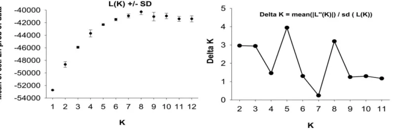
Figure 2.2. Estimated population structure of Astyanax cave and surface population using STRUCTURE for
K = 2 and K = 5 population.
Figure 2.3.A. Proportion of shared alleles between the studied populations shown as Euclidian distances.
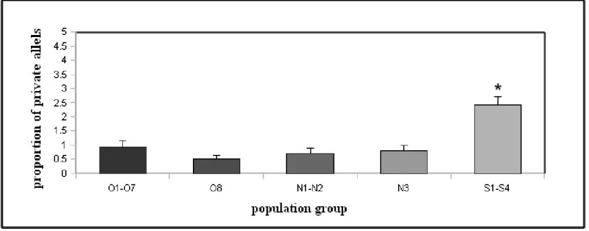
Figure 2.3.B. Private allelic richness averaged over geographically grouped populations.
Figure 2.4. Estimates of effective population size (Ne) based on Bayesian inferences of migration rates and
population sizes among Astyanax mexicanus population.
Figure 2.5. Summary of the estimates of gene flow based on Bayesian inferences of migration rates and
population sizes using MIGRATE-N 3.2.6.
Figure 2.6. Correlations between genotype and phenotype in three mixed cavefish populations.
Figure 3.1. Summary of Astyanax contig statistics using RAD tag sequencing methodology.
Figure 3.2. Integrated linkage maps (microsatellite + SNPs) of Astyanax mexicanus with colored bars
denoting positions of detected QTL for specific trait.
Figure 3.3. Distribution of the percentages of total (PEV) and additive (PEVad); variance explained (PVE) at
the phenotypic loci per each trait on the QTL map as identified using MultiQTL.
3.4.A. PCA for all the SNP markers used in the study.
3.4.B. PCA for SNPs produced by RAD tag and Sanger sequencing method for the markers with MAF > 5%
in surface populations.
Figure 3.5. Trends in heterozygosity for different marker panels.
Figure 3.6. Distributions of the outlier loci in multiple cave vs. surface comparisons.
Figure 3.7. Summary of the differentiated loci detected by hierarchical outlier test per each population.
Figure 3.8. Correlation between single locus FST estimates from outlier loci test vs. observed
heterozygosities (Ho) in multiple cave-surface comparisons.
Figure 3.9. Correlation between single locus FST estimates from outlier loci test vs.FIS (inbreeding coefficient)
in multiple cave-surface comparisons.
Figure 3.10. Proportion of the loci out of HW equilibrium.
Figure 3.11. Observed marker numbers of markers per each population and linkage group.
Figure 3.12. LD versus physical distance between SNPs for three population panels: Surface (SN1), old
population (O1) and new population (N2).
Figure 3.13. Summary of the outliers found inside or outside the population per each population.
Figure 3.14. Haplotypes and population comparisons of the different QTLs and linkage groups.
Figure 3.15. Representation of the 800kb of Danio rerio region of ZV8 assembly on the chromosome 13
homologous with the QTL region in LG3.
6
Figure S2.1. A detailed hydrological map of the El Abra region with the indication of surface and subsurface
water divide.
Figure S2.2. Estimates of gene flow based on Bayesian inferences of migration rates and population sizes
using MIGRATE-N 3.2.6 among Astyanax mexicanus population clusters within each geographical region.
Figure S2.3. Summary of the proposed models.
Figure S3.1. SNP only map of Astyanxa mexicanus with colored bars denoting positions of detected QTL for
specific trait.
Figure S3.2. Minor allele frequencies in each population.
List of Tables
Table 1.1.A. Examples in which similar phenotype evolved within a species by different genetic changes.
Table 1.1.B. Examples in which similar phenotype evolved within a species by similar genetic changes.
Table 2.1. Sample information and summary statistics of the sampled populations.
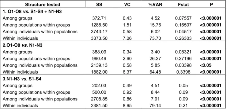
Table 2.2. Analyses of molecular variance (AMOVA) in cave and surface populations for 26 microsatellite
loci.
Table 2.3. Multilocus pairwise FST estimates from 26 microsatellite loci in Astyanax mexicanus.
Table 3.1.A. Summary and description of the measured phenotypes, abbreviations and their mean values in
F2 generation as measured by Protas.
Table 3.1.B. Summary of identified QTL with their respective linkage groups, position, maximum LOD score
and P-values.
Table 3.2. Details on sample locations, population abbreviations, origin, sampled individuals (N), and marker
quality control per populations.
7DEOH*HQHWLFGLYHUVLW\IRUWZRPDUNHUJURXSV³FDYH613V´DQG³VXUIDFH613V´PDUNHUVDQGDYHUDJHG parameters per populations.
Table 3.4. Summary of significant FST values assigned to the QTL locus.
Table 3.5. Summary of the gene list with their functions and positions from the region on the Chr 13 in Danio
rerio which shows synteny with cavefish.
Table S3.1. Summary of identified QTL with their respective linkage group position and maximum LOD
score.
7
Acknowledgements
First and foremost I want to thank to my supervisors Dr. Richard Borowsky and Dr. Henrique Teotónio. They gave me enormous support and great opportunities through all these years of my PhD. I am thankful for their excellent model as a scientist and above all as a people. I thank Dr. Borowsky for sharing his enormous knowledge about this extraordinary organism-Mexican blind cavefish as well as possibility to do the fieldwork and learn a lot about caving and caves. Henrique deserves special thanks for giving me a great opportunity to work in his lab as pre-doctoral student. He gave me enormous support through all this years of my career.
I would like to thank to my colleagues from GABBA PhD program, especially to the 10th edition. It was a great scientific and personal experience to be a student in this great environment. I would also like to thank Prof. António Amorim as a director of the GABBA 10th edition as well as our program secretary Catarina Carona for her efficacy and great help with solving any administrative problems through all these years.
8
I would also like to thank to our collecting expedition team; Geoffrey Hoese and Jean Luis Lacaille Muzquiz, Paco and Sarai and all the other people that provided enormous help during my fieldwork.
I want to thank all the members of Teotónio lab (Evolutionary genetics group) at the IGC that have contributed immensely not only to this thesis but also to my personal time at the IGC. They have always been a source of great mood as well as excellent scientific discussions. I thank Sara for being a great ³YL]LQKD´, friend and a colleague during all this time and especially during the very intense period of writing this thesis. I would also like to thank Bruno for being a great colleague and translating my summary to Portuguese. Dr. Ivo Chelo should probably get at least 10 pages of acknowledgments for his support during my data analysis and fruitful discussions during all these years. ,RZHKLPDQHQRUPRXV³thank you´IRUEHLQJSDWLHQWZLWKP\programming as ZHOODVIRUVKDULQJKLVVFULSWVDQG³5´NQRZOHGJHZLWK me.
I thank Isabel Marques and Joao Costa for sharing their experiences about genotyping and providing great technical support during my experimental work at the IGC.
,ZDQWWRWKDQNP\JUHDW³,*&IULHQG´5LFDUGR, for a great friendship and scientific discussions during my time at the IGC. My dearest friends Nadja and Liliana, there are no words I could possibly use to tell how much I am thankful for all these years of friendship, support and sharing the same stages of the scientific career in good and bad moments on the both sides of the ocean -. You guys are the greatest friends ever!
At the end, the biggest thank you goes to my parents and my sister that have been supporting me all these years wherever I was and wherever I have decided to go.
9
Summary
10
cave populations than in related surface populations due to their smaller effective population sizes, probably because of limitations in food and space. However some of the cave populations receive migrants from the surface and exchange migrants with one another, especially when geographically close. This admixture results in significant heterozygote deficiencies at numerous loci due to Wahlund effects. In cave populations receiving migrants from the surface, we identified small numbers of individuals that are both phenotypically and genotypically intermediate between the cave and surface forms, affirming gene flow from the surface. Our study confirmed that the cave populations are GHULYHGIURPWZRPDLQVXUIDFHVWRFNVWKDWZHFDOO³ROG´DQG³QHZ´SRSXODWLRQV and that diverged about 6.7 Mya, based on estimates from a previous study. ³1HZ´FDYHSRSXODWLRQVDUHFORVHUWRWKHVXUIDFHSRSXODWLRQVZKLOH³ROG´FDYH SRSXODWLRQV DUH PRUH GLVWDQWO\ UHODWHG WR VXUIDFH DQG ³QHZ´ SRSXODWLRQV ,Q addition to that, our results suggest the old stock surface populations inhabited at least three independent cave localities while there are two independent ORFDOLWLHV LQKDELWHG E\ ³QHZ´ VWRFN VXUIDFH SRSXODWLRQV 7KXV ZH KDYH HVWDEOLVKHGHYROXWLRQDU\FRQYHUJHQFHWKDWUHIHUVWRFKDQJHVEHWZHHQ³ROG´DQG ³QHZ´SRSXODWLRQVDQGSDUDOOHOHYROXWLRQDU\V\VWHPWKDWUHIHUs to the changes between the populations within each of these groups. This part of the study clearly established the relationship between the phenotypically similar populations and allowed us to further investigate the importance of natural selection in the parallel and convergent evolution.
In the second part of the thesis we developed and genotyped 745 SNP markers in multiple cave and surface populations and further asked: can we find loci that were repeatedly selected for in the cave environment? All together, 80 loci were identified in several independent populations and they are potentially involved in adaptation to the cave environment.
11
physical genome of cavefish is not available we integrated our information with the data from laboratory crosses. We used an F2 cross between the cave and
surface individuals and genotyped the same SNP markers in the F2 progeny.
This allowed us to design a genetic map. Measures of 10 phenotypic traits that differ between cave and surface populations were available from previous studies. We used quantitative trait loci analysis (QTL) in essence correlating genotype with phenotype, to detect regions in the genome with gene loci that are responsible for each phenotype.
Some of the 80 SNPs detected as adaptive in multiple natural populations also mapped to the QTL loci for lens, amino-acid sensitivity and eye size. Those SNPs were then joined into haplotypes. Some of these haplotypes denoting SXWDWLYHVHOHFWLRQZHUHIRXQGRQO\LQ³QHZ´FDYHSRSXODWLRQVEXWRWKHUVZHUH IRXQGERWKLQ³QHZ´DVZHOODV³ROG´FDYHSRSXODWLRQV
Our study supports the hypothesis that convergent adaptive phenotypic change in different populations can arise through a conserved genetic basis (shared haplotypes in new and old cave populations). Furthermore, we observed the alternative possibility that implies that natural selection can repeatedly generate similar patterns of phenotypic variation in totally novel ways (haplotypes in only new cave populations).
12
Resumo
A compreensão da base genética da variação fenotípica adaptativa é central para podermos compreender a origem e a manutenção da diversidade biológica. A ocorrência sistemática dos mesmos fenótipos em populações geneticamente próximas ou distantes constitui uma técnica muito poderosa para testar o papel da seleção natural na sua manutenção. A investigação da base genética por detrás das semelhantes alterações fenotípicas constitui a melhor oportunidade de unificar ideias bem estabelecidas sobre a extensão dos constrangimentos que existem nas alterações evolutivas. Será que fenótipos semelhantes se diferenciam sob semelhantes bases genéticas ou será que a seleção usa várias vias genómicas alternativas que convergem nas mesmas soluções fenotípicas? Estas alterações ocorrem principalmente com base na variação genética já existente no genoma ou será dependente de novas mutações? Nesta dissertação abordámos estas questões de forma integrada usando diferentes populações do peixe cego das cavernas mexicano (Astyanax mexicanus) como modelo e tirámos partido das ferramentas da genética populacional, genética quantititativa e da genómica.
Esta espécie é única, com trinta populações diferentes em cavernas que derivaram de populações da superfície. Existem também várias características fenotípicas que diferenciam as formas das cavernas das formas da superfície, que incluem a redução pigmentar e do tamanho dos olhos, hipertrofia dos órgãos sensoriais não ópticos, taxa metabólica mais reduzida, o número de papilas gustativas e de costelas, bem como várias diferenças a nível comportamental. Em primeiro lugar perguntámos quantas vezes estas características morfológicas evoluíram de forma independente nas populações das cavernas.
13
e 26 loci de microssatélites em segregação independente. As populações de grande parte dos locais à superfície são geneticamente semelhantes, com algumas excepções, enquanto as populações das cavernas estão geneticamente diferenciadas e têm pelo menos cinco origens nas três regiões principais. Encontrámos uma menor diversidade genética nas populações das cavernas relativamente às populações da superfície relacionadas devido ao menor tamanho efectivo das primeiras, o que por sua vez se pode justificar pelas limitações de alimento e de território. Contudo, algumas das populações das cavernas receberam migrantes da superfície e trocaram também migrantes entre si, sobretudo quando geograficamente próximas. Esta mistura resulta em deficiências significativas de heterozigotas em numerosos loci
14
seleção natural na evolução paralela e convergente.
Na segunda parte da tese desenvolvemos e genotipámos 745 marcadores de SNPs em múltiplas populações de superfície e de caverna e perguntámos: podemos encontrar os loci que foram repetidamente selecionados no ambiente cavernícola? Em suma, 80 loci foram identificados em várias populações independentes e estão potencialmente envolvidos na adaptação a este ambiente.
Seguidamente, perguntámos onde se posicionavam estes marcadores no genoma e se coincidiam com a região envolvida nas características fenotípicas. Uma vez que o genoma físico do peixe cego das cavernas mexicano não está disponível, integrámos a nossa informação com dados de cruzamentos no laboratório. Usámos a geração F2 de cruzamentos entre
indivíduos das cavernas e da superfície e genotipámo-la, procedimento que nos permitiu obter um mapa genético. As medições de 10 fenótipos que diferenciam estas populações estavam disponíveis através de um estudo anterior. Utilizámos posteriormente uma análise de loci de caracteres quantitativos (QTL), essencialmente para correlacionar genótipos e fenótipos e detectar os loci no genoma responsáveis por cada fenótipo.
15
16
CHAPTER 1
INTRODUCTION
A suite of structural, functional and behavioral changes of the organism generally accompanies adaptation to a new environment and these processes have been the subjects of scientific inquiry for a long time. However the mechanism of these changes in the natural populations remain largely unknown: :KDWDUHWKH³ORFLRIDGDSWDWLRQ´UHVSRQVLEOHIRUWKHHPHUJLQJRIWKH new morphological traits? How many loci are responsible for a particular trait of interest and how repeatable is evolution if the same morphology evolves multiple times from the same or divergent ancestors? What are the underlying evolutionary mechanisms that drive these changes?
17
phenotypes occur thorough changes in the same or different genetic loci. Due to the good surrogate for the ancestral phenotypic state (surface fish) there is also a good reason to ask if the adaptations to the novel environment are the result of new mutations or preexisting genetic variation in an ancestral population.
This thesis addresses the above-mentioned questions and focuses on assessing the relative contributions of different evolutionary forces; gene flow, and natural selection and different source of variation; new mutations and preexisting genetic variation, to the evolution of similar phenotypes in independent populations.
1.1. Convergence and Parallelism: similar or different ways to the same trait?
Definitions
18
convergence [1] (pp. 78±79) [11, 12] (e.g. wings in birds and bats).
However, when focusing on two biological levels- phenotype and genotype- within the simplified framework of parallel and convergent changes these definitions are much more complex. There has been lot of debate in the field in order to establish common terminology for convergence and parallelism taking both phenotypic and genotypic observations into account [13, 14]. Parallel evolution is often difficult to differentiate from convergence and some authors have even suggested a continuum between convergent and parallel evolution [13, 15, 16]. The distinction between convergent, parallel, and divergent evolution indeed requires the historical evolutionary aspect of studied lineages.
19
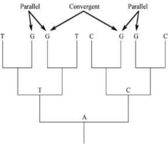
Figure 1.1. Parallelism vs. convergence in molecular evolution. Character states at a single nucleotide site
are mapped onto a gene tree. Parallelism refers to the independent evolution of the same derived state from
a common ancestral state (the two Gs from T, or the two Gs from C). In contrast, convergence involves the
evolution of the same derived state from different ancestral states (G derived independently from T and C)
(adapted from [2]).
How did unrelated species or populations evolve to look so similar?
Evidences from experimental evolution
Repeated patterns of phenotypic traits are commonly regarded as evidence of adaptation under common selection pressures such as common environmental factors [5, 17-23]. Despite the scientific profundity of this question, as well as the exceptional utility of convergent and parallel evolution for teaching us about adaptation and natural selection, relatively little is known about the genetics behind phenotypic similarity.
20
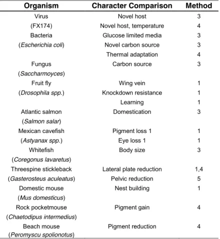
to examine the extent and dynamics of molecular changes during adaptation [27]. Replicate lineages were adapted to growth at high temperature on either of two bacterial hosts. The researchers then documented the extent to which convergent evolutionary changes occurred during this period. They found that more than half of the 119 observed nucleotide substitutions were the same. Some of these molecular changes were host-specific, and others were found in phages growing on both hosts. There are more evidences that phenotypic shifts in such a simple organisms result frequently in minor sequence changes and a single locus accounts for the entire response to selection [25, 28] (Table 1.1 A).
21
Organism Character Comparison Method
Virus Novel host 3
(FX174) Novel host, temperature 4
Bacteria Glucose limited media 3
(Escherichia coli) Novel carbon source 3
Thermal adaptation 4
Fungus Carbon source 3
(Saccharmoyces)
)UXLWÀ\ Wing vein 1
(Drosophila spp.) Knockdown resistance 1
Learning 1
Atlantic salmon Domestication 3
(Salmon salar)
Mexican FDYH¿VK Pigment loss 1 1
(Astyanax spp.) Eye loss 1 1
:KLWH¿VK Body size 3
(Coregonus lavaretus)
Threespine stickleback Lateral plate reduction 1,4
(Gasterosteus aculeatus) Pelvic reduction 5
Domestic mouse Nest building 1
(Mus domesticus)
Rock pocketmouse Pigment gain 4
(Chaetodipus intermedius)
Beach mouse Pigment reduction 4
(Peromyscu spolionotus)
Method of Comparison: 1 = hybrid complementation; 3 = patterns of gene expression; 4 = sequencing of candidate genes; 5 = phenotypic comparison.
Table 1.1.A. Examples in which similar phenotype evolved within a species by different genetic changes.
22
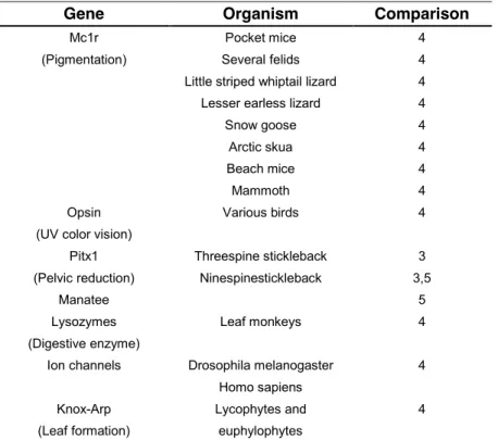
Method of Comparison: 1 = hybrid complementation,3 = patterns of gene expression; 4 = sequencing of candidate genes; 5 = phenotypic comparison.
Table 1.1.B. Examples in which similar phenotype evolved within a species by similar genetic changes.
Adapted from [13].
Evidences from natural populations
The genes that are the direct targets of selection for producing similar phenotypes have been identified in only a handful of natural systems. Some of the best examples in natural populations come from different fish populations with clearly established phylogenetic relatedness between different populations. For example, two eco-morphs of the lake whitefish (Coregonus clupeaformis), one dwarf (smaller, more limnetic) and other normal (benthic), are found in northeastern North America. They have evolved rapidly, independently and in parallel in different freshwater lakes [30-37]. Parallel
Gene Organism Comparison
Mc1r Pocket mice 4
(Pigmentation) Several felids 4
Little striped whiptail lizard 4
Lesser earless lizard 4
Snow goose 4
Arctic skua 4
Beach mice 4
Mammoth 4
Opsin Various birds 4
(UV color vision)
Pitx1 Threespine stickleback 3
(Pelvic reduction) Ninespinestickleback 3,5
Manatee 5
Lysozymes Leaf monkeys 4
(Digestive enzyme)
Ion channels Drosophila melanogaster 4
Homo sapiens
Knox-Arp Lycophytes and 4
23
expression patterns have been identified and strongly suggest a role of natural selection in genes that are related to energetics. Another example represents genotype-phenotype association of the vision genes in cichlids. Mutation and expression in opsin genes has demonstrated parallel adaptation to a different water depth by divergent selection in Lake Victoria [38].
Finally, the most studied example comes from sticklebacks, which are interesting fishes in that they lack scales and instead have armour plating. From a highly plated marine ancestor, in numerous freshwater environments armour plating is reduced or lost repeatedly and independently after colonization. Most freshwater populations have low-plate Eda alleles arguing for a strong role of repeated, independent positive selection in freshwater environments from standing genetic variation [4, 39, 40]. Recent genome-wide study of adaptive loci sticklebacks has also shown Eda, as well as multiple other regions involved in adaptive process to freshwater environment [5, 31].
Besides the parallel genetic changes within the species those conserved changes are also apparent when comparing different species. An example of that is the adaptation of the color in the beach mice. The change in coloration is due to the exact same amino acid polymorphism in Mc1r gene that is also found in a population of wooly mammoths (Table 1.1B). Surprisingly, in the beach mice there is also a possibility that different genes from that melanin production pathway can produce the same phenotypic change (Table 1.1A and B) [4-6, 9, 10, 41]. Also, an interesting example of convergent evolution of the wing color switch genes in two different butterfly species was also described recently [42-46].
24
developmental constraints cause limitations to a few alternative phenotypes [2, 8, 13, 24, 45, 47]. Other researchers provide evidences of attaining the same phenotype via different genetic changes even among closely related taxa (Table 1.1A). These studies suggest that if multiple developmental pathways can lead to the same phenotype, then parallel evolution is a signal of adaptation [48]. Most of these studies are based on little empirical data, since the genome wide screen of adaptive variation in natural populations was not available till recently. Thus, it remains unclear to what extent natural selection or genetic drift can facilitate parallelism and convergence on genome-wide level. Natural selection will be at least partially responsible for repeated evolution of the same trait in association with the similar environmental change [5, 17, 49-51]. Genetic drift will also play a role in repeated phenotypic evolution, but the phenotypic transitions will probably not be linked to the environment consistently. Because of that, occurrence of the repeated phenotypes is one of the best tools to test natural selection in the wild [18, 50, 52].
change-25
from standing genetic variation? What do distantly related populations/species tell us about that processes? Is there any rule?
There are not many studies that address the importance of standing genetic variation vs. new mutations even in model species (reviewed in [53]). The reason for the low number of studies is probably because standing genetic variation is most reliably distinguished from de novo mutation by sampling of the ancestral and derived population. Thus, a suitable natural system that affords access to both ancestral and derived states is required (reviewed in [59]). Also, until recently it was impossible to sample enough polymorphism in non-model organisms to allow for this kind of study.
Many studies, either in the lab or in nature, point out a huge importance of standing genetic variation in the process of adaptation to the new environments. For example, adaptation from standing genetic variation in replicated populations in experimental evolution in Drosophila has shown that adaptation to a new laboratory environment largely occurs from the sorting and recombination of standing genetic variation at multiple loci [58]. In natural populations only one study tests the allele frequency change from standing genetic variation tracking Eda genotype frequencies over a multiple generation in stickleback populations. The low frequency beneficial allele present in ancestral population increased in frequency very fast over multiple generations [39, 54, 55, 59]. Recent genome wide studies or sticklebacks and whitefish also suggest that most of the adaptive variation is present in a very low frequency in the ancestral population [5, 31].
1.2. Astyanax Mexicanus as a model to test convergent and parallel
evolution
26
morphological form (cave and surface) sets an excellent opportunity to study the genetic and evolutionary mechanisms of convergent and parallel evolution. Repeated appearance of the same phenotype in the group of cave organisms is also very common, especially following the repeated multiple independent colonization of caves by the surface ancestral phenotypic form which frequently result in eye regression like in cave amphipods [61, 62] and cavefish [63-67]. Organisms existing in such circumstances often result in a suite of changes called troglomorphy; progressive elongation of body form and appendages as well as an increase in sensory structures, hypertrophy of nonoptic sensory organs and a reduced metabolic rate [68-70]. Cave animals represent one of the best examples of convergent evolution and offer some unique advantages for studying its mechanisms.
One of the best-studied taxa is the teleost Astyanax mexicanus, a fish species that includes both eyed surface and eyeless cave-dwelling populations [64, 65, 67]. The first Mexican cave characin was described in 1936 by Hubbs and Innes as Anoptichthys jordani. In the mid-1960's, as a result of activities by members of the Texas-based Association for Mexican Cave Studies in the Sierra de El Abra many different localities with the cavefish populations have been discovered. Cavefish was first described as three species (Anoptichthys jordani, A. antrobius, and A. hubbsi, respectively). Nowadays, we are taking about unique genus with the inter-fertile surface and cave forms and they are considered as morphotypes of the same species, Astyanax mexicanus [63, 65]. Multiple trips and studies of Sierra de El Abra followed and today we know of 29 cave populations of Mexican blind cavefish [65]. One of the pioneering studies to address the origin of different cavefish populations was a cross between two JHRJUDSKLFDOO\ LVRODWHG FDYH¿VK SRSXODWLRQV WKDW UHVXOWHG LQ )1
27
study showing minimal divergence in 17 allozyme loci concluded that the Sierra de El Abra cavefish had a common origin [63]. In contrast, Mitchell et al. who surveyed 29 different cavefish populations in the Sierra de El Abra, Sierra de Guatemala, and Micos region, proposed several different origins of Astyanax cavefish [65]. Cavefish is thus an attractive model to study genetic basis of independently evolved morphological traits.
Evolutionary history
28
Figure 1.2. Map showing the region containing 29 different Astyanax cDYH¿VK SRSXODWLRQVLQ QRUWKHDVWHUQ 0H[LFR7KHVSKHUHVLQGLFDWHWKHDSSUR[LPDWHSRVLWLRQRIFDYHVZLWK$VW\DQD[FDYH¿VK7KH*XDWHPDOD(O Abra, and Micos clusters are indicated on the map. Inset: Mexico showing the northeastern region indicated
in the sketch map (shaded rectangle) and the outlying Guerrero population (shaded sphere). Adapted from
Jeffery [79]. Annu.Rev.Genet.43: 25-47.
Morphological changes in Astyanax mexicanus
29
the morphs themselves also vary to a large degree. For example, the caves have different amounts of water and numbers of pools; therefore the size of the population will vary significantly. Caves can also be connected with the surface rivers or completely isolated, with consequences for the degree of troglomorphy attained by the populations, especially eye and pigmentation reduction [65, 67]. Phenotypic similarity between different cave morphs might mask mechanistic or developmental differences, making the classification of phenotypic evolution dependent on the level of organization being studied. However, although the similarity to ancestral forms can vary from exact features to mere approximations, the novel pathways and forms used to accomplish these similarities are what make studies of morphological evolution worthwhile.
Candidate gene approach
30
reveal that many candidate genes that are differently expressed between morphs, nevertheless it is still impossible to conclude which genes are the main causes of morphological change. Therefore additional genetic resources were necessary in the study of this organism.
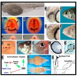
Figure 1. 3. Summary of phenotypes and expression studies in Astyanax Mexicanus. (A) Albinotic Pachón
cavefish embryo with melanin positive melanoblasts after l-DOPA supplementation. (B, G) Surface fish
embryo with eye primordium (F), and adult with eye (H). H, I) Pachón cavefish embryo with small eye
primordium showing a reduced ventral sector (F), and eyeless adult (G). (H±K) Cavefish embryos show
expanded shhA expression along the midline and contracted pax6 expression in the eye fields. (H, I) Surface
fish. (J, K) Pachón cavefish. (H, J). Neural plate stage viewed dorsally. (I, K) Ten somite stage viewed
rostrally. Markers (dlx3) indicate the border of the neural plate and (pax2) boundary of the future midbrain
and hindbrain region in the neural plate. (L, M) Overexpression of shh induces lens apoptosis (L) and a blind
cavefish phenocopy (M) in surface fish. (N) Transplantation of a lens from an embryonic surface fish into the
optic cup of a Los Sabinos cavefish rescues eye development. (O, P) Sections through embryonic surface
fish and Pachón cavefish eye primordia showing apoptosis in the cavefish (P) but not the surface fish (O)
lens. Arrows in (P) indicate the lens (L) and retina (R). (Q) Diagram showing effects of expanded Hh
signaling in cavefish. (R) Comparison of brain morphology in surface fish and cavefish. Dorsal views with
anterior on the left. (S) Differences in bottom feeding posture in surface fish and cavefish. (A) is reproduced
31
Quantitative trait analysis (QTL) studies in Astyanax mexicanus
Most species studied for ecological or physiological traits lack genomic data and A. mexicanus is no exception. Even in the absence of a genome sequence this species became an exceptional model to study the genetic basis of morphological traits due to its amenability to genetic and QTL analyses [70, 76-78, 80]. The map was assembled using 259 markers to detect recombination frequencies and testing association of 12 traits that differ between cave and surface tetras (eye size (E), melanophore numbers (M), body condition rate (C), number of maxillary teeth (T), sensitivity to dissolved amino acids (A), rate of weight loss (W), body length (L), depth of the caudal peduncle (D), the placement of the dorsal fin (P), size of the SO3 dermal skull bone (S), numbers of anal fin rays (R), ribs number (B) [77]. Presence of numerous multi-traits QTL on the map such as EMT, EMCTW and EMRDS is very surprising given that these traits are not functionally related.
The QTL map of the other two crosses with Tinaja and Molino cave morphs with surface fish is also in the finishing state. According to preliminary data it is evident that the QTL maps while integrated do not map at the same positions as in Pachón, which supports the idea of independent evolution of the traits in the different caves [93]. Furthermore, crosses between geographically isolated cavefish populations (Molino, Pachón, and Tinaja) can produce progeny with a greater degree of eye development than that exhibited by either parent [67, 75].
32
candidate genes (Cg1, Fbp, Gh, Igf1, Igfbp5, Ins, Tfe3, Idh2, Oca2, Pax6, Shh, and Twhh were also placed on the map [77, 78, 81]. The phenotypic changes, even though much less studied also include constructive changes like increased complexity of feeding apparatus (larger jaws, mechano-sensory system (more taste buds, larger cranial neuromasts), and a more sensitive olfactory system and modified behavior patterns.
In addition to the conventional forward genetic approaches to better understand eye and pigmentation regression, some recent studies focused on behavioral changes associated with the cave environment. These experiments identified both sleep patterns and sensitivity to vibration as very important adaptations also observed in a multiple populations [94, 95].
Impact of natural selection in the adaptation of cavefish phenotypes
The impact of natural selection on cave evolved organisms and their regressive traits remains one of the most interesting questions. The neutral mutation hypothesis [96] was largely proposed for the eye regression in
Astyanax mexicanus. It was suggested that given enough time and a sufficiently high mutation rate random mutations in eye-forming genes accumulate in cave animals under relaxed selective pressure [67, 97, 98]. Thus, eyes would eventually disappear because they are not necessary for survival in the dark environment. On the other hand adaptation theory attributes eyes regression to energy economy. Also, pleiotropic effects have been proposed in which sensory organs beneficial to survival in the cave environment are enhanced at the expense of eyes [77, 93, 99].
33
showed that reduction of eye and of pigmentation occurred independently [77]. Therefore different evolutionary mechanisms could control regression of these traits. QTL assignment test that tests QTL polarity showed consistent polarity of all eye QTLs. This suggests that natural selection might be driving evolution of those loci. If both natural selection and drift are involved in the evolution of those traits, the QTL polarity should randomly change as it was observed for pigmentation QTL. These studies thus proposed natural selection driving eye loss as a main energy conservation mechanism. Contrary to that it was hypothesized that in pigmentation regression neutral mutation was the driving force [77]. However, the relationships between neutral mutation and selection are very poorly understood in Astyanax FDYH¿VK DQG IXUWKHU UHVHDUFK RQ
multiple natural populations is needed to clarify them.
1.3. Quantitative genetics approach in detecting genetic basis behind morphological traits
Another approach to detecting parallel or convergent genotypic adaptation in non-experimental systems involves quantitative genetic analysis (QTL). The major interest of QTL study lays in the identification of regions in the genome that harbor loci affecting complex trait variation and estimating the magnitudes and polarities of effects due to allelic variation at these loci in the experimental population.
34
QTL is a powerful approach that allows us to ask many important questions in the evolution of morphological traits [8, 102, 104-106, 109]. For example, how many loci are responsible for the given trait and how much variance in phenotype may be explained by each locus? Are the loci of small or large effect? Are there interactions between the loci (epistatic effect) or are multiple traits encode by the same genes (pleiotropy)?
QTL studies are primarily used in model species because they are easiest to perform. For example, in Drosophila melanogaster, many genetic markers have been developed and the flies are easy to breed and maintain in the laboratory, which makes QTL analysis easier [110-112]. Nevertheless, QTL mapping had a lot of success in identifying genetic basis of morphological traits even in some non-model systems [6, 9, 78, 113, 114]. For example, stickleback marine and freshwater populations are radically different in their morphology; using QTL studies, multiple QTL were detected that controlled the numbers of gill rakers, lateral plates, pelvic spines, etc. [4, 6, 7, 9].
QTL mapping in non-model species is frequently combined with a search for candidate genes causing similar phenotypes in model species [78, 80, 115-117]. For example, a combination of genetic mapping and candidate gene determination was very successful in discovering the causes of albinism, alterations in the structure of melanin, and decreases in the numbers of melanophores in Astyanax mexicanus [78, 80]. Combination of QTL and candidate genes was also used in the QTL study to identify the genes and mutations responsible for morphological change in cave adapted isopod (A. aquaticus). Those genes fall into area of the genome responsible for presence
vs. absence of pigmentation phenotype. However, the candidate genes were not causative once, but they are rather linked to the causative loci [118].
35
that is that fine scale QTL mapping is a prolonged and costly process of narrowing a QTL to a region with few enough candidate genes that each can be thoroughly tested. This ability to reduce QTL to a small number of testable candidate genes is necessary for increasing the rate at which QTLs are identified and proven. Thus, studies ideally need to combine both QTL and population genomics approach [5, 31, 32, 42, 44, 46, 119, 121].
Traditional linkage mapping is useful for identifying rare alleles and is not subject to the effects of population structure. However, loci that are identified by QTL mapping are specific to the parental lines of the experimental segregating populations and may not be representative of the genetic variation on which natural selection acts.
1.4. Inference of evolutionary history and demographic processes in the natural populations
36
statistical independence among populations may be misplaced. Thus, when assessing adaptive phenotypic differentiation, the structure of evolutionary relationships among populations must be considered [128-130].
To understand maintenance of variation with species and importance of local selection and demography, determination of population parameters such as genetic distance, gene flow, population structure and effective population size is very important [131-133]. In particular, it is important to examine whether patterns of adaptive morphology observed within populations are replicated across the natural range of the species. This information will allow us to ask the following question: Are those phenotypes derived from a single event followed by dispersal, or if they are adapted multiple independent times? Is there a gene flow between the independently derived lineages? In other words, do adaptive phenotypes have a single evolutionary history (parallelism) or they appeared by convergence (from the distantly related lineages)? Having this information it can be determined when and under what circumstances phenotypic variations has evolved and separate recent selective events from historical processes.
Population structure
Despite the success of population genetics in modeling neutral variation, many assumptions of these predictions are frequently violated in natural populations, which make the estimation of genetic parameters a challenging task. One of the very important aspects of describing demographic effects is to determine population substructure and gene flow. This information is necessary for accurate estimates of effective population sizes (Ne), genetic diversity, and
37
geographic region may mate with each other; and as such, they cannot be accounted for easily [130, 134] [123, 133]. Clearly, it is impossible to model the full biological complexity of demographic events, so we must look for the simplest models that capture the relevant features. Typically, we ask the question: How can we detect deviations from the null model and how can we estimate some of the important quantities related to the demographic models?
Population structure separates individuals into distinct reproductive units. Each of these units may behave like an ideal population Wright-Fisher population; finite size, where each individual contributes an infinite number of gametes to a gamete pool, and then each member of the next (finite) generation is drawn from that gamete pool) [135]. Over time, the stochastic nature of the evolutionary process will lead to genetic differentiation between populations; different allele frequencies among the populations or even complete fixation of different alleles in different populations. For example, if there was a locus with two alleles in multiple sub-populations, each with the frequency pi; the expected average heterozygosity (He) in the combined
population under Hardy-Weinberg equilibrium (HWE) would be 2p (1-p), where p represents average allele frequency [136]. However, because of the reproductive isolation between these sub-populations, the heterozygosity will be reduced by the amount of allele frequency variance across sub-populations. This variance in allele-frequency is directly related to the population inbreeding; the frequency of heterozygotes compared with that expected when genotypes are in HWE. Also, inbreeding increases relatedness between the LQGLYLGXDOVEDVHGRQFRPPRQDQFHVWU\³LGHQWLW\ E\GHVFHQW´LEG [137]. Thus population structure can be defined as ibd and it can be measured as relatedness between the individuals relative to the populations and between populations relative to the species. These measures were proposed by Wright and are termed F-statistics with the different hierarchical levels denoted as FIS
38
mating within a subpopulation; i.e. genetic inbreeding within subpopulations), FST (the mean reduction in heterozygosity of a subpopulation relative to the
total population due to genetic drift among subpopulations; i.e. between-population differences) and FIT (mean reduction in heterozygosity of an
individual relative to the total population) [128, 137-139].
:ULJKW¶V)VWDWLVWLFVPHDVXUHWKHFRUUHODWLRQEHWZHHQDOOHOHVGUDZQDW different levels of a subdivided population [139, 140]. Evolutionary processes, such as mutation, migration, inbreeding, and natural selection influence that correlation. The original definition of F-statistics was to measure the amount of allelic fixation owing to genetic drift.
:ULJKW¶VFST model is an idealized n-island model in which an infinite
number of populations receive immigrants from an infinitely large mainland population [141]. FST is a simple function of effective population size and the
migration rate FST = 1 / (1+4Nem) in which the strength of genetic drift is
SURSRUWLRQDOWR1ZKLOHWKHVWUHQJWKRIJHQHÀRZLV proportional to m. When FST = 0 there is no differentiation between the populations, when FST = 1
differentiation is maximum.
Levels of population differentiation are typically quantified using a YDULDQWRI:ULJKW¶VFST parameter, which measures the proportion of variation in
a sample that is distributed among populations. This has been the most used approach, partly because of its robustness and partly because it is simple to implement [139]. This estimator of FST can give us a good idea about what
form of demographic model may apply to the data.
However, the relationship between real demographic parameters and FST are
not so simple. FST is a very good estimate of the population differentiation;
however the estimates of FST should not be directly translated into Ne x m;
measure of gene flow. The reason for that is that the relationship of the variance in gene frequencies among different populations (FST) is related to the
non-39
equilibrium demography typically increases the variance of summary statistics, highlighting the importance of using simulations to study power and efficiency of this approach [143].
Population genetic theory [144-146] has allowed for the development of more robust methods to measure population structure including coalescent-based likelihood methods (where likelihoods are estimated by stochastic simulation) and Bayesian methods [128, 147, 148]. These methods account for more of the underlying biology of populations. For example, they give insights into the rates of mutation and migration; because of that they provide more information on population structure than FST summary statistics [128, 129].
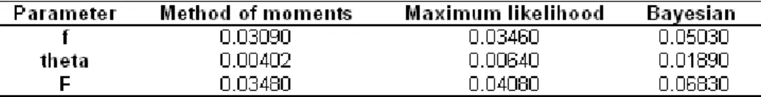
Estimates of FST using the method of moments and Bayesian methods
have not been extensively compared. An example of the differences among calculating method of moments, maximum-likelihood and Bayesian estimates of F-statistics has been shown by Holsinger & Weir [128]. They used a study on human populations in which the allele frequency differences at blood group loci were measured (Table 1.2). Based on this example it has been suggested that those differences in estimates are small under the following conditions: when the average number of individuals per population is moderate to large (>20), when the number of populations is moderate to large (>10±15) and when most populations are polymorphic.
f-Coancestry for alleles within an individual relative to the subpopulation in which it occurs; equivalent to Fis; theta- Coancestry for randomly chosen alleles within the same subpopulation relative to the entire population; equivalent to FST;
F-Coancestry for alleles within an individual relative to the entire population; equivalent to Fit.
Table 1.2. Differences among calculating method of moments, maximum-likelihood and Bayesian estimates
of F-statistics. Data from a classic study on human populations that investigated the allele frequency
40
However, when the assumption of uniform effective population sizes (Ne) and symmetric migration rates assumed by summary statistics is violated,
there is big discrepancy between the above methods and parameter estimates. This is especially evident in populations with high Ne [149, 150] that are weakly
structured, and when highly polymorphic molecular markers are used for the structure detection [151]. An example of that is reported in the estimation of the population structure of big eye tuna populations. In this study Bayesian cluster analyses, and coalescence-based migration rate inferences supported high migration rate and lack of genetic structure, which contrasts the FST estimates
[152].
Population history and demography also has an important role in the mode (balancing and directional selection; see description latter) and efficacy RI QDWXUDO VHOHFWLRQ )RU H[DPSOH ORZ OHYHOV RI JHQH ÀRZ HQKDQFH ORFDO adaptation [153]. On the other hand, efficacies of positive and negative selection are reduced in populations with small effective sizes or those that experienced severe bottlenecks [123]. Given those effects, the details of the demographic processes are not only important for the null model against which selection will be tested, but they are also very important for the appropriate models of selection.
1.5. Selection detection in the natural populations
locus-41
specific effects help identify genes that are important for fitness and adaptation and will often reveal different patterns of variation (reviewed in [157]). Selected loci could be detected based on reduced diversity, excess of linkage disequilibrium (discussed later) within and among populations, haplotype structure, fixed DNA sequence divergence among related taxa or high geographic differentiation relative to the other loci across the genome.
Besides detecting selected loci it is also very important to distinguish between the modes of the selection present in the surveyed region. The modes of selection that are commonly identified in the natural populations either operate on the mean value of the trait (balancing selection) or on the one extreme of the trait distribution (positive selection). The actions of selective forces are than reflected in the allele-frequency of the adapted populations [155]. Balancing selection causes multiple alleles to be maintained in a population, often at fairly constant frequencies [158]. In the case of positive VHOHFWLRQIDYRUDEOHPXWDWLRQEHFRPHV¿[HGLQDSRSXODWLRQ
Different tests for selection are designed to find different departures IURP³QHXWUDO´GHPRJUDSKLFPRGHOVLQFHDOOGHPRJUDSKLFFRPSOH[LWLHVFDQQRW be taken into account, as discussed before. In the other words, there is no VXFKDWKLQJDV³SHUIHFWWHVW´IRUVHOHFWLRQ+RZFDQZHPDNHVXUe than that we have identified selected locus? Repeated detection of the same loci by different statistical methods could be one of the solutions. Another possibility is to investigate biological replicates that inhabited different environments and experienced the change in selective pressures, which will have a strong power to understand genome-wide adaptation. Here, we are presenting approaches for selection detection that are commonly used in non-model systems [155, 159].
Outlier detection
42
with the ability to screen numerous markers in genome scans to identify candidate genes for further investigation. In general, these methods consist of identifying loci that differ from expectations under the neutrality based on summary statistics (FST and homozygosity). The power to distinguish outlier loci
from neutral loci is dependent on the null distribution of the summary statistics across the genome. The null distribution can be experimentally obtained by collecting hundreds of loci. However, in non-model system it is rare to have so many loci, thus simulations to model neutral loci are frequently used [154, 160-162].
The problem is therefore to generate the distribution of statistics under demographic model congruent with the observed data. The models that are used in outlier tests can involve different population structures and histories and can assess the influence of different demographic and non-equilibrium scenarios. These models are robust to a wide range of alternative demographic models. It is likely that they will detect outliers with unusually high or low FST and will identify selection at one or many loci through pairwise
comparisons of populations [154, 156, 157, 163-166]. The basic rationale for testing natural selection using these methods is that loci influenced by positive selection will show a larger genetic differentiation than neutral loci (high FST).
On the other hand, loci that have been subject to balancing selection will show a lower genetic differentiation (low FST). However, outlier tests typically
generate discrepancies when numbers of immigrants per generation are unequal, the true population history consists of repeated branching events, or the connectivity of populations is uneven [167-169]. These discrepancies are mostly reflected in limited power in detecting balancing selection. Isolation, population bottlenecks, and heterogeneity of populations are also increasing the possibilities to detect false positive or negative loci [154] as well as weak divergent selection [170].
43
where the selected loci were defined. They showed different sensitivity to detect balancing selection. Again, accurate detection of balancing selection is an inherent weakness of outlier approaches. A similar conclusion was reached in the recent study of adaptation in natural populations of sticklebacks [169]. This study used multiple outlier tests in order to compare selected loci across the methods. They were able to consistently indentify the same loci across the multiple methods. However, loci under balancing selection showed major issue of the methods. Both of these studies point out that statistical methods should be carefully chosen based on the purpose of the study with special attention to the error rates of the different methods [168].
Linkage disequilibrium and haplotype based tests
44
These classical definitions of LD are very important and widely used, but its patterns are well known for being noisy and unpredictable. For example, two pairs of markers can be in complete disequilibrium even when they are unlinked whereas LD for the pair of markers next to each other might be weak (reviewed in [176]). Also, these statistics consider only two loci at a time, whereas we may be interested to calculate the extent of LD across a chromosome segment that contains multiple markers. LD in genotypic data can be quantified [178, 180], but the lack of information about the haplotype phase weakens the signal of nonrandom association sufficiently that this approach is not often taken. Haplotypes are not known in unrelated individuals and they have to be inferred, which is easily done based on frequencies from the genotypes in the surveyed populations [181]. They are typically more informative than individual genotypes, when LD between the phased markers is strong. The strength of haplotypes is in the usage of multiple SNPs together (haplotype blocks) while estimating population genetic parameters [177, 182, 183]. Thus, it is more common to use a statistical method based on population genetics theory to infer haplotype phase from genotypic data and then to treat the inferred haplotypes as if they were data.
Haplotype diversity can be the result of migration, mutation, selection, small finite population size (eg. [108] and those effects can be inferred using many different methods [155, 158, 182-184]. For example, we can measure haplotype diversity using a count of the number of observed haplotypes in a region or by the expected haplotype heterozygosity based on haplotype frequencies in a region [176, 177]. One of the simplest approaches when data for more than one population are available is to partition the haplotypes into contributions within and among populations. This partitioning first suggested by Ohta [174, 175] and it LVVLPLODUWR:ULJKW¶VVWDWLVWLFVWKDWSDUWLWLRQVYDULDELlity within the populations (FIS) and between the populations (FST) (for explanation
45
the specific haplotypes in the population that diverged from the other haplotypes, just like the single outlier SNP (reviewed in [176]). If the natural selection favored adaptation to local conditions we will detect increased FST
whenever alleles at different loci are favored [156, 157]. Partitioning haplotypes in different regions in the genome is an appropriate step when trying to determine whether differences in haplotype frequencies result from natural selection stemming from differences in conditions among populations.
Integrative approach in detecting adaptive loci behind repeated phenotypes
In the past few decades LD has been also utilized as a tool for genetic mapping of trait or disease loci in the natural populations [172, 173, 176, 186]. Mapping based on LD requires alleles to be in LD with an allele responsible for a quantitative trait, across the entire population. To be a property of the whole population, the association must have persisted for a considerable number of generations, so the marker(s) and causative locus must therefore be closely linked. LD mapping and its variations (e.g. association mapping, selective sweep mapping) are commonly used approaches in finding genes that underlie ecologically important traits in natural populations [143, 172, 176, 177, 183]. These approaches rely on a statistical association between genotype and phenotype, and have shown great potential for fine mapping of traits and for identifying functional markers [171, 173, 186-188].
46 statistical power) [189].
Unfortunately, due to the unknown positions of the markers in the genome these studies are not very common in natural systems. A successful example of similar approach (only individual SNPs were used instead of haplotypes) that combined individual markers from natural populations survey with QTL from experimental crosses was given by Rogers and Bernatchez [32]7KH\FRPELQHGSRSXODWLRQVFDQVRIWKHJHQRPHIRU³RXWOLHU´ORFLZLWK47/ mapping to examine the genetic basis of growth rate differences between limnetic and benthic ecot\SHVRIZKLWH¿VK%\SHUIRUPLQJ47/PDSSLQJXVLQJ AFLP markers that were previously used in population genomics scans [31, 190] they were able to determine that the loci closest to growth rate QTL were the same as loci showing elevated differentiation in genome-wide scans of natural populations. Combinations of genome-wide scans and traditional QTL mapping allows for testing whether QTLs identified in different populations have played a part in adaptive phenotypic differentiation. This is clearly a powerful tool in non-model organisms in which physical genome is not available [8, 31, 42, 44, 46, 106, 155].
1.6. Objectives
Identification of the causative polymorphisms underlying parallel and convergent phenotypic traits and understating the evolutionary forces driving that change is an extremely challenging task in organisms, which lack extensive sequence information and genomic resources. The main goal of this work was to contribute to the general understanding of the evolutionary mechanisms underlying phenotypic evolution in natural populations using a non-model organism from the following perspectives:
47
independent microsatellite markers across different populations.
48
CHAPTER 2
Gene flow and population structure in the Mexican blind
cavefish complex (
Astyanax mexicanus
)
RUNNING TITLE: Demography of cavefish and surface conspecifics
Submitted manuscript
*Adapted from
Martina Bradic1, 2, Peter Beerli3, Francisco J. García-de León4, Sarai Esquivel-Bobadilla4, Richard L.
Borowsky1
1Cave Biology Group, Biology Department, New York University, NYC, NY, USA
2
Univesidade Nova de Lisboa, Oeiras, Portugal
3
Department of Scientific Computing, Florida State University, Tallahassee, FL, USA
4
Centro de Investigaciones Biologicas del Noroeste (Laboratorio de Genética para la Conservación), La Paz,
49
2.1.
SUMMARY
50
2.2.
BACKGROUND
The mechanisms underlying the evolution of similar phenotypes in independent natural populations pose a long-standing question in evolutionary biology. Apart from a few examples [191, 192] the molecular nature of convergent phenotypes remains largely unknown. Also unknown is the extent to which new mutations versus preexisting genetic variation in ancestral populations contribute to convergence (or parallelism) [4, 193].
Convergence is of interest to evolutionists for several reasons, one of the most important of which is that it provides an element of replication to evolutionary studies that is often otherwise absent. Replication allows for the powerful testing of evolutionary hypotheses. Cave-dwelling organisms provide the best known examples of convergences, sharing similar phenotypes such as loss of eyes and pigmentation across diverse taxonomic groups [194].
The Mexican blind cavefish (Astyanax mexicanus) is nearly unique among cave animals because the cave forms have closely related surface conspecifics and the two forms are fully interfertile [67]. The ability to hybridize the cave and surface forms permits the genetic analysis of the factors involved in cave adaptation. There are 29 known cave populations of this species dispersed over a broad geographic range and the group may present multiple examples of convergence.
Each population inhabits a food and light restricted cave environment; their members exhibit numerous cave-related evolutionary changes, including reduction in pigment and eye size, hypertrophy of non-optic sensory organs, increased condition factor, and robust patterns of reduced sleep; presumably all are evolved in response to reduced food availability in caves [65, 67, 76-78, 94].
51
evolutionary questions, including the extent to which morphological, behavioral and physiological evolution is driven by selection versus drift [79, 81, 97]. These two alternatives can be distinguished in a number of ways in this system, but any determination will require an understanding of the underlying demography of the populations as well as a clarification of the relationships among them.
Previous phylogeographic studies of Astyanax cavefish, using microsatellite and mtDNA, showed that the cave populations are derived from at least two different surface stocks that inhabited the Sierra de El Abra and nearby regions in succession [71-74]. The estimates from mtDNA suggest that these two groups diverged about 6.7 Mya [72]. Surface forms of the older stock originally inhabited the rivers in the El Abra region and were the likely ancestors of a series of cave populations, which ZH GHVLJQDWH DV ³ROG´ Subsequently, the surface fish of the old stock went locally extinct. The region was then invaded by another stock of A. mexicanus; its descendants are the FXUUHQW RFFXSDQWV RI WKH UHJLRQ¶V VXUIDFH ZDWHUV DQG D VHFRQG VHW RI FDYH SRSXODWLRQVZHGHVLJQDWHDV³QHZ´
52
Figure 2.1. Map of the Sierra de El Abra region showing all the cave and surface collection sites. Colored
lines delineate major geographical regions (labeled below), as follow: El Abra region: O1 ± O8 (blue & green
circles); Guatemala region: N1 ± N2 (red circles); Micos region: N3 (purple circles); Surface localities S1 ±