Econ. Apl. vol.12 número3

(1)

Marcelo L. Moura§ Adauto R. S. Lima¤

Rodrigo M. Mendonça†

rEsumo

O desempenho de previsão para fora da amostra é testado para um amplo conjunto de modelos empíricos de taxa de câmbio em uma economia emergente com taxa de câmbio flutuante e regime de metas de inflação. Comparado à literatura recente de modelos de previsão da taxa de câmbio, nós incluímos um conjunto mais extenso de modelos. São testados modelos tradicionais da década de 1980, modelos de equilíbrio comporta-mental da taxa de câmbio dos anos de 1990 e um modelo baseado na regra de Taylor. Neste último, o modelo incorpora um função de reação do Banco Central, na qual a taxa de juros é definida de acordo com uma regra de Taylor. Nossos resultados demonstram que modelos de regra de Taylor e de equilíbrio comportamental da taxa de câmbio, este último combinando diferenciais de produtividade com ajustes de carteira, têm desem-penho fora da amostra superior a um passeio aleatório. Evidências de poder de previsão também são obtidas para modelos parcimoniosos baseados em argumentos de paridade descoberta da taxa de juros.

Palavras-chave: modelos de regra de Taylor, modelos monetários, previsibilidade fora da amostra, cointe-gração, modelos de correção de erros.

aBstract

Forecasting performance is tested for a broad set of empirical exchange rate models for an emerging economy with independently floating regime and inflation target monetary arrangement. Compared to the recent literature on out-of-sample exchange rate predictability, we include a more extensive set of models. We test vintage monetary models of the 1980’s, exchange rate equilibrium models of the 1990’s and a Taylor Rule based model. This last model assumes an endogenous monetary policy, where the Central Bank follows a Taylor rule reaction function to set interest rates. Our results show that Taylor Rule models and Behavioral Equilibrium Exchange Rate models, the last one combining productivity differentials with portfolio balance effect, have superior predictive accuracy when compared to the random walk benchmark. Some out-of-sample predictability is also obtained with parsimonious models based on uncovered interest parity arguments.

Keywords: Taylor rule models, monetary models, out-of-sample exchange rate predictability, cointegration, mean correction error models.

JEL classification: F31, F41, F47.

* We would like to thank an anonymous referee, participants at the 7th Brazilian Finance Meeting and at the 15th World Congress of the International Economic Association for their very helpful comments on previous versions of the paper. All possible remaining errors are ours

§ Ibmec São Paulo – Business School. Adress contact: Rua Quatá 300, São Paulo – SP – Brazil – CEP: 04546-042. E-mail: marcelom@isp.edu.br.

¤ Ibmec São Paulo – Business School. Adress contact: Rua Quatá 300, São Paulo-SP – Brazil – CEP: 04546-042. E-mail: adautorsl@isp.edu.br.

† Ibmec São Paulo – Business School. Adress contact: Rua Quatá 300, São Paulo – SP – Brazil – CEP: 04546-042. E-mail: rodrigomm1@ibmecsp.edu.br.

(2)

1 introduction

In the present study, we test the adequacy of the empirical exchange rate models for an emerging commodity-based economy with independently floating regime.1 Our purpose is to assess the out-of sample fit of those models. Our analysis replicates for an emerging economy the study carried out in the classic article by Meese and Rogoff (1983) but with a broader set of economic models and using true out-of-sample exercises.2 The original Meese and Rogoff work showed that a simple driftless random walk model would be more effective for the ex-change rate forecasting than the models that involve macroeconomic fundamentals.

Meese and Rogoff’s research has generated an extensive literature. Mark (1995) argues that the monetary fundamentals might obtain some success to explain the behavior of the exchan-ge rate if the statistical tests were given more power. However, a host of authors, for example, Kilian (1999) and Berkowitz and Giorgianni (2001) remained skeptics and suggested that the results obtained by Meese and Rogoff may still seem robust, even after all the data and intense academic investigation gathered for over twenty years.

Some exceptions to this skepticism are present in recent works. Chen (2004) analyzes commodities producers (Australia, Canada and New Zealand) for OCDE countries. The au-thor concludes that for Australia and New Zealand the global price of their respective exported commodities is likely to have a meaningful and stable impact on their respective currencies. However, in the case of Canada, the evidence was less conclusive.

Guo and Savikcas (2006) make use of variables that reflect the agents’ expectation to-wards the future behavior of the economic fundamentals, like the term structure of interest rates, credit risk, and the idiosyncratic risk of the United States’ stock market, among others. Their analysis suggest that the idiosyncratic risk of those assets forecast the American dollar’s behavior facing the G7’s main currencies, and conclude that the exchange rate does not follow a driftless random walk..

Cheung, Chinn and Pascual (2005) added other models and elements of the 1970s tradi-tional specifications in the determination of the exchange rate, such as, the net foreign assets and the differential of relative productivity in the tradable goods sector between countries, the Balassa (1964) and Samuelson (1964) effect. The authors concluded that, in line with a great part of the existing literature, it is very difficult to find empirical estimations of structural models that may consistently outperform a random walk, having the mean-squared errors as basis of comparison. On the other hand, the structural models provide a better forecasting for exchange rate movements than that provided by the random walk.

1 This definition follows the exchange rate arrangements adopted by the IMF, and available at http://www.imf.org/ external/np/mfd/er/index.asp

(3)

Specific studies for Brazil, like Muinhos, Alves and Riella (2003), state that the random walk is not the best hypothesis to explain the behavior of the exchange rate in Brazil. Using data from May 1999 to December 2001, the authors conclude that a model derived from the theory of uncovered interest rate parity captures the Brazilian exchange rate’s behavior better. This model takes into consideration the sovereign risk premium (in the study measured by the C-Bond spread, in relation to Treasury Bills, as a variable in the specification of the uncovered parity.

Until mid 2000’s, as highlighted by Sarno and Taylor (2002), though the theory of exchan-ge rate determination had produced a series of models, estimations both in and out- of-sample did not show strong empirical support. The results tended to be fragile in the sense that they were hard to replicate in different samples or countries. However, new developments in the mid 2000’s changed the perspective and shed some new light in the field.

Engel and West (2005) analysis of rational expectations present-value model showed that beating a random-walk can be a too strong benchmark, even if the model is true. At the same time, the use of endogenous monetary models, see Molodtsova and Papell (2007), and new panel data techniques, see Rapach and Wohar (2004) found improved results in out-of-sample predictability. As a recent paper from Engel, Mark and West (2007) suggests in his title: “Ex-change Rate Models are not as Bad as You Think”.

In conclusion, the existing literature up to now allows us to draw some important conclu-sions. First of all, it is difficult to find empirical economic models that consistently outperform a driftless random walk for the out-of-sample estimations. Second, more recent exchange rate models improve the predictive accuracy of the models. Finally, economic variables that have forward-looking components may improve the results of the models for the out-of-sample fore-casting.

(4)

2 spEcification of thE modEls

The Flexible Price Monetary Model (FPMM) was very representative in the 1970s when the floating exchange rates were adopted by the main industrialized economies, after the collapse of Bretton Woods system in 1973. According to Sarno and Taylor (2002), this model became the dominant exchange rate model during the 1970s, for earlier studies on this see Frenkell (1976) and Mussa (1976, 1979).

The basic intuition of the FPMM is to assume that, in each country, the equalization of currency supply and demand determines the price level in each country. Furthermore, relative prices in each country and exchange rates are related by the purchasing power parity rela-tionship. The solution of the FPMM leads to an exchange rate equation where the exchange rate is determined by relative money supplies, output levels and interest rates. More specifically, in econometric terms, the equilibrium equation to be estimated can be presented by:

(

) (

)

0 1 2 4

t t t t t t t t

s = β + β m −m∗ + β y −y∗ + β i −i∗ +v (2.1)

where s_tis the exchange rate logarithm (R$/US$), m_tand m_t* the M1 logarithms in Brazil and in the United States, respectively; y_tand y_t*the industrial production logarithm in both coun-tries and i_tand i_t* the logarithm for the short-term interest rates for Brazil and the United States, respectively.3 The variable v_t is a random term.

Despite the fact that the FPMM was the dominant approach to determine the exchange rate in the early 1970s, its weak empirical results led to the conception of models that took over frictions in the economy, inducing another form of convergence for long-run market equili-brium. Dornbusch (1976) introduces the idea of sticky prices in the short run to the exchange models, which enables jumps in the nominal and/or real exchange rate to beyond its long-run equilibrium value. The existence in the system of variables that jump, in this specific case, the exchange rate and the interest rate, would make up for the stickiness in other variables, that is, the prices of goods. Thus, the adjustment velocity in various markets would be different.

Consider π_t and π_t∗ as logarithms of the inflation rates in Brazil and in the United States respectively. The Dornbusch (1976) SPMM, captures price stickiness in both economies by the following equilibrium equation:

(

) (

)

0 1 2 4 5

t t t t t t t t t t

s = β + β m −m∗ + β y −y∗ + β i −i∗ + β π − π + ν∗ (2.2)

where νtis a random term.

The monetary models formerly shown, flexible prices and sticky prices, assume the perfect substitution between home and external assets and their effects on the exchange rate. However,

(5)

the existence of home-bias (home agents’ preference for home assets), liquidity difference, sol-vency risk, tributary differences and even the currency-exchange risk can affect the presumed equilibrium in the monetary models, which makes the home assets and the external assets imperfect substitutes.

Following Sarno and Taylor (2002), the main idea in the Portfolio Balance Model - hereaf-ter PBM - is to consider that net financial wealth can be allocated into money, domestic issued bonds and foreign bonds. At the equilibrium, exchange rate and nominal interest rates equate supply and demand of those three financial assets. In the reduced-form, the equilibrium ex-change rate will be a function of relative money supplies and the stock of domestic and foreign bonds.

Most of the empirical estimates of the PBM showed poor results, see Bisignano and Hoo-ver (1982) and Dooley and Isard (1982). HoweHoo-ver, longer data span and estimation for an emer-ging economy, like the Brazilian, motivates us to test this model as well. In particular, we use the following empirical specification for the portfolio model:

(

) (

)

*

0 1( ) 2 3 4 5

t t t t t t t _t t t t

s = β + β m −m + β i −i∗ + β ngd −ngd∗ + β embi + β nfa +v (2.3)

where the additional variables ngd_t is the logarithm of the net government debt to GDP, inter-nal plus exterinter-nal less internatiointer-nal reserves, embi_t is the country risk sovereign spread meas-ured by the EMBI+ Brazil4, nfa_t is the logarithm of the public sector dollar denominated net foreign assets. Asteriks denote the same variables for the reference country, the United States.

The next specifications follow a more recent set of exchange rate determination models model in the Balassa-Samuelson tradition. Following Cheung, Chinn and Pascual (2005) we use first a productivity Differential model where the productivity gap between tradable and nontradables sectors play a crucial role in determining the equilibrium exchange rate. The Pro-ductivity Differential is given by the following equation:

(

) (

)

0 1 2 4 5

t t t t t t t t t t

s = β + β m −m∗ + β y −y∗ + β i −i∗ + β z −z∗ + ν (2.4)

where z_tgives the logarithm of productivity ratio of the tradable to the nontradable sector, which is measured by the respective inverse price level ratios of each sector.

Besides the Balassa-Samuelson effect, we can also include other well-known familiar effects to the exchange rate in order to establish a link between the exchange rate and the re-levant economic variables. That is exactly the idea of Clark and MacDonald (1999) Behavior Equilibrium Exchange Rate Model – hereafter BEER. More specifically, the BEER model

(6)

assumes a reduced form econometric specification where the real equilibrium exchange rate is affected by transitory factors, random disturbances, and the extent to which the economic fundamentals are away from their sustainable values.

In our specification of the BEER model, we followed closely the specification used in Cheung, Chinn and Pascual (2005). The set of explanatory variables includes the relative price of nontradables, ϖ_t, the real interest rate differential, *

t t

r −r , net government debt to GDP ra-tios, ngd_t−ngd_t∗, terms of trade, tot_t and net foreign asset position, nfa_t:

(

)

* *

0 1 2( ) 3 4 5

t t t t t t t t t t t

s = β +p −p + β ϖ + β r −r + β ngd −ngd∗ + β tot + β nfa +v (2.5)

We also test a parsimonious model based on uncovered interest rate parity (UIP) condi-tions. This model has been extensively tested in the literature with poor results, see Hodrick (1987) for survey results. However, recent studies pointed to more hope for the UIP models, for instance, Flood and Rose (2002) show that UIP models tend to work better using more recent data from the 1990s, Chinn and Meredith (2004) using a larger span of data and incorporating long-term interest rate differentials also achieve better in-sample estimates for the UIP.

Given that an emerging economy is subject to many risks not captured by the interest rate differential, we assume two flexible functional forms. The first assumes that the exchange rate will be a function of short term interest rate differentials,

(

)

0 1

t t t t

s = β + β i −i∗ + ν (2.6)

while a second specification includes the country-risk, measure by the EMBI+ index men-tioned earlier:

(

)

0 1 2

t t t t t

s = β + β i −i∗ + β embi + ν (2.7)

As pointed out by Engel, Mark and West (2007), two important characteristics of moneta-ry policy were ignored up to now. First, it is endogenous. Second, since the mid-1980s central banks have used interest rate as the instrument policy, not money supply. Therefore, our last model incorporates endogenous monetary policy set by the definition of the short-term interest rate according in the spirit of Taylor (1993) central bank reaction function. Following the line of New-Keynesian monetary models, we apply a Taylor Rule model. The Taylor model for exchange rate determination was employed recently by Engel and West (2006), Mark (2007), Clarida and Waldman (2007) and Molodtsova and Papell (2007).

In general, monetary policy rules are summarized by a Taylor’s rule function:

1 1

t q t t t y t t mt

(7)

We assume γ > γ > γ >_q 0, _π 1, _y 0, 0≤ δ <1. For the foreign country:

1 1

t t t y t t mt

i∗ = γ_πEπ + γ∗₊ y∗+ δi∗₋ +u∗

Using the two Taylor Rules above with the uncovered interest parity condition:

*

1

t t t t t t

i −i =E s₊ − + ρs

where ρ_tdenotes a risk-premium and E_t the conditional expectations conditioned on time t information, we can write:

(

) (

)

*

0

1 1 1 1

1 1

( 1) ( ) ( )

j j

t t t t t t j

q

t t t t t y t t t t mt mt t

q s p p b b E f

b

f E E y y i i u u

+∞

= +

∗ ∗ ∗ ∗

π + + − −

≡ − + = ∑

≡ + γ

 

= − γ −_ π − π + γ − + δ − + − −ρ _

In particular, using the last expression we can specify this model by the following econo-metric equation:5

(

) (

)

(

)

* *

0 1 2

*

3 4 5 1

( ) ( ) ( ) ( )

( ) ( )

t t t t t

s PDV y PDV y PDV PDV

PDV i PDV i embi q₋ v

= β + β − + β π − π

+β − + β + β + (2.8)

where ( ) 0

j j

t t t j

PDV x ≡ ∑b +∞₌ b E x₊ denotes the present value of expected future variables. For the Taylor Rule Model we used historical expectations from the Consensus Forecast Econom-ics Survey using a value of b=0,9.6

3 out-of-samplE forEcasting

3.1 Cointegration diagnostic tests

A general expression for the relation with the exchange rate is:

0

t t t

s = β + Χ Π + e (3.1)

5 The lagged term for the real exchange rate accounts for the serial correlation of the exchange rate and the relative price level difference,p p*

t− t

6 This value was obtained by direct estimation of it= γqqt+ γπEtπ + γt+1 yyt+ δit−1+umt for Brazilian data and using

1 (1 _q)

(8)

where X_t denotes the vector of explanatory variables, Π is a vector of parameters and e_t is a random term. Since many of the macroeconomic variables are not stationary, we need to test if [ ,s X_t _t] has a long-run relationship in order to avoid spurious regressions. Following the seminal work of Engle and Granger (1987) we test if [ ,s X_t _t] co-integrate by using MacKin-non (1991) critical values for the Engle-Granger two-step procedure.

Empirical estimation uses monthly data from January 1999 to December 2007, a full sample of 108 observations.7 Using the full sample, we first estimate (2.1) to (2.8) and generate the estimated residuals series,eˆ_t, for each model. Then, we run the regression:

1 ˆ_t ˆ_t₋ u_t

∆e = α + γe + (3.2)

and test for the null of no-cointegration of γ =0. As pointed out by Engle and Granger (1987), t-statistics for γ under the null will have no standard distribution, depending on the sample size and the number of parameters. For this reason, we use MacKinnon (1991) critical values.

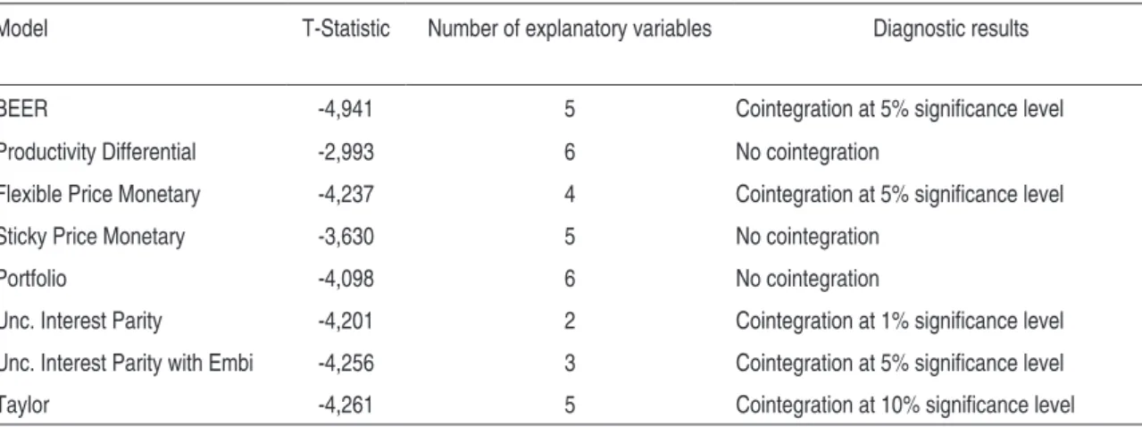
Results for the Engle-Granger cointegration tests are presented on Table 1. They show that the Productivity Differential, the Portfolio and the Stick Price Monetary models does not cointegrate. This means that specifications (2.2) to (2.4) do not produce meaningful estimates leading to spurious regressions. However, we will keep those models in our forecasting exer-cise just for scientific curiosity to evaluate if we can obtain any predictive accuracy of them, the theory should say that we will not.

(9)

Table 1 - Cointegration tests for the Exchange Rate Models

Model T-Statistic Number of explanatory variables Diagnostic results

BEER -4,941 5 Cointegration at 5% signiicance level

Productivity Differential -2,993 6 No cointegration

Flexible Price Monetary -4,237 4 Cointegration at 5% signiicance level

Sticky Price Monetary -3,630 5 No cointegration

Portfolio -4,098 6 No cointegration

Unc. Interest Parity -4,201 2 Cointegration at 1% signiicance level

Unc. Interest Parity with Embi -4,256 3 Cointegration at 5% signiicance level

Taylor -4,261 5 Cointegration at 10% signiicance level

Note: Asymptotical critical values obtained from MacKinnon (1991) assuming a no-trend statistics corresponding to equation (3.2).

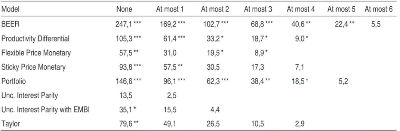
The cointegration tests on Table 1 assume that there is only one cointegration relationship. A more general alternative, given the presence of many macroeconomic series in our models, would be to test for the presence of multiple cointegration relationships.8 Table 2 presents re-sults of the Johansen (1991) VAR-based cointegration tests. For the Taylor and the Uncovered Interest Parity with EMBI models, Johansen’s tests confirm the result of the Engle-Granger test and presents just one cointegration relationship. However, for some other models there is evi-dence of more than one cointegration vector. In particular, we fail to reject the null of at most one cointegration equation for the following models: BEER, with evidence of four cointegration relationship at 1% significance level and six at 5%; productivity differential, two at 1% and four at 10%; sticky price monetary, two at 5% and portfolio, three at 1%, four at 5% and five at 10% .

This last result suggests the use of Vector Error Correction models for those models. How-ever, the drawback of using VEC in forecasting at long horizons is the need of including short-term dynamics of the explanatory variables. For instance, Groen (2000) uses the VEC approach in order to estimate a monetary model and forecasts up to 4 years ahead. However, information about the values of the short-run dynamics for years 1, 2 and 3 ahead are not available at time t. If we want true ex-ante forecasts, some sort of VEC modeling without the short-run dynamics is necessary for true forecasts and we leave this topic for future research.

(10)

Table 2 - Johansen Cointegration Tests - trace statistics

Model None At most 1 At most 2 At most 3 At most 4 At most 5 At most 6

BEER 247,1 *** 169,2 *** 102,7 *** 68,8 *** 40,6 ** 22,4 ** 5,5

Productivity Differential 105,3 *** 61,4 *** 33,2 * 18,7 * 9,0 *

Flexible Price Monetary 57,5 ** 31,0 19,5 * 8,9 *

Sticky Price Monetary 93,8 *** 57,5 ** 30,5 17,3 7,1

Portfolio 146,6 *** 96,1 *** 62,3 *** 38,4 ** 18,5 * 5,2

Unc. Interest Parity 13,5 2,5

Unc. Interest Parity with EMBI 35,1 * 15,5 4,4

Taylor 79,6 ** 49,1 26,5 10,5 2,9

Note: Johansen cointegration tests were based on the assumption of a constant and no trend in the estimation equa-tion. Asterisks ***, **, * denote rejection of the null at 1%, 5% and 10% significance levels.

3.2 Forecasting exercise

The out-of-sample forecasting analysis followed the mean correction error methodology used by Cheung, Chinn and Pascual (2005). Firstly, we estimate specification (2.1) to (2.8) as represented by equation (3.1), obtaining the fundamental value for the exchange rate:

0 ˆ ˆ

t t

F = β + Χ Π (3.3)

The second step is to estimate the following mean correction equation:

( )

t k t t t t

s₊ − = φs F −s +v (3.4)

The estimated parameters of equation (3.4) are used to forecast future values of the ex-change rate at the horizons of k = 1, 3, 6 and 12 months ahead. Notice that, using (3.4) we avoid the problem of using future unknown explanatory fundamentals to predict the exchange rate. In our exercise, only information available at time t is used to estimate the future exchange rate.

We used the technique of rolling regressions on (3.4). Initially, we estimated (3.1) using data from January 1999 through October 2005, a total of 70 observations. Then, for each estimated model, we made one-, three-, six- and twelve-month projections ahead for the exchange rate level. At a second moment, we displaced, using the rolling regression method, the estimation of the models one period ahead, keeping the size of the initial sample. We repeated the procedure to the exhaustion of the sample. This procedure is then compared with the forecasting of a mo-del that assumes the exchange rate following a drift less random walk, that is:

t k t

(11)

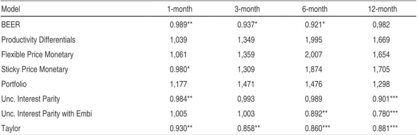
Table 3 displays Theil’s ratio between the Root Mean Squared Error9 (RMSE) of each specification and the RMSE of the random walk. To test the statistic significance of this ratio, we used the statistic proposed by Clark and West (2006, 2007), in which, under null hypothesis, there is no difference between the two estimations forecasting performance. That is, the fore-casting generated by the economic models is as good as the forefore-casting generated by a driftless random walk. Thus, numbers inferior to one indicate that the economic models outperformed a driftless random walk for the out-of-sample forecasting of the exchange rate n-periods ahead; numbers superior to one indicate that the economic models underperformed a driftless random walk.

Table 3 - RMSE ratios

Model 1-month 3-month 6-month 12-month

BEER 0.989** 0.937* 0.921* 0,982

Productivity Differentials 1,039 1,349 1,995 1,669

Flexible Price Monetary 1,061 1,359 2,007 1,654

Sticky Price Monetary 0.980* 1,309 1,874 1,705

Portfolio 1,177 1,471 1,476 1,298

Unc. Interest Parity 0.984** 0,993 0,989 0.901***

Unc. Interest Parity with Embi 1,005 1,003 0.892** 0.780***

Taylor 0.930** 0.858** 0.860*** 0.881***

Note: RMSE ratios are defined as model RMSE divided by random-walk RMSE, values lower than one indicate that the economic model had a better out-of-sample performance than the random walk. Asterisks ***, **, * denote rejection of the null at 1%, 5% and 10% significance levels.

As expected by the theory, models that presented better out-of-sample predictability are the ones that co-integrate the exchange rate and macroeconomic fundamentals. In particular, the best forecasting performance is obtained using the BEER and Taylor models. Interestingly, a parsimonious model based on uncovered interest parity also shows a satisfactory forecasting accuracy, especially for 6 and 12 month-ahead horizons.

Figures 1 and 2 plots the random walk and competing models forecasts compared to ac-tual exchange rates for 6-month and 12-month-ahead forecasts. From the graphs we can see many interesting aspects. First, all models capture the exchange rate appreciation of the end of 2004 to December 2007. Second, the random-walk guess, which is the same exchange rate series displaced six or twelve months-ahead is a good forecast and hard to beat. Third, although all models are able to predict an appreciation trend from 2004 to 2007 their estimated exchan-ge is almost always above its actual value. Fourth, the major deviations of the predicted and

9

2 ˆ

( )

1 N _s _s

t t t RMSE

N − ∑ =

(12)

estimated values are in general at the beginning of the forecasting window, during 2005 and 2006. Exceptions are the models that had RMSE ratios significantly lower than one in Table 3, namely, the Taylor model and the UIP with EMBI at six and twelve-months-ahead forecast, and the BEER model at six-months ahead forecast.

3.3 Data discussion

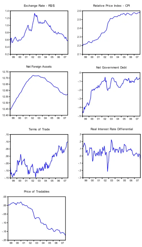
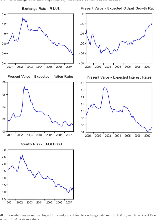
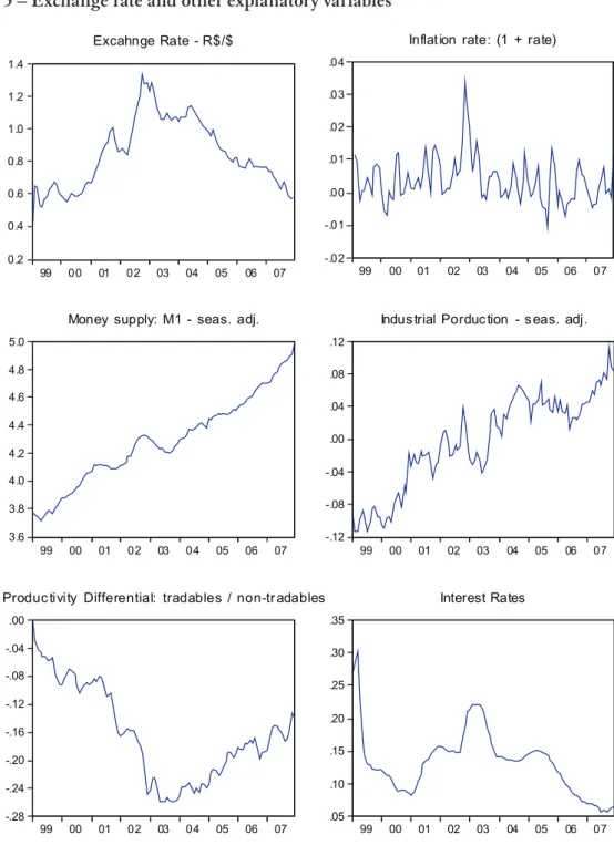
Given the strong predictability results of the BEER and Taylor models, we find useful to discuss the most relevant series.10 Figure 3 presents the exchange rate and the explanatory variables for the BEER model while Figure 5 does the same for the Taylor model. Figure 6 presents the remaining explanatory variables used on other models.

Looking first to the exchange rate series, we see clearly two distinct periods. From 1999 to 2003 the real/dollar exchange rate has clear tendency towards depreciation and from 2003 to 2007 the tendency is reversed to an appreciation movement. This movement coincides with the confidence crisis in the Brazilian economy during 2002, justified by investor’s uncertainty about the presidential elections during that year, the favoritism and posterior victory of the left-wing government.

For the BEER model, however, it is not only about investor’s and political uncertainty. From 1999 to 2002, the macroeconomic fundamentals already pointed to a depreciation ten-dency. In Figure 3, we can see this by looking at the 1999-2002 upward movement on the rela-tive price index, net foreign assets and net government debt. After 2002, the new elected gover-nment strongly signals for a conservative monetary and fiscal policy, and net govergover-nment debt and relative CPI prices stabilizes. In response to external favorable conditions, we also verify a decrease in net foreign assets, explained by foreign domestic investment and current account surpluses, and the improvement of terms of trade. In conclusion, worsening in inflation levels, net government debt and increase in net foreign assets in 1999-2002 explains the depreciation movement; afterwards, stabilization of inflation and debt, decrease of net foreign assets and external favorable conditions in terms of trade and price of tradables appreciated the currency.

Compared to the BEER model, the Taylor model uses a different approach to explain the movement of exchange rates during the 2001 to 2007 period.11 Figure 4 shows clearly the strong depreciation in 2002 motivated by an equally sharp deterioration of expectations in terms of lower growth rates, higher inflation rates and a country risk increase. In response, we see a pos-terior increase in expected interest rates at the end of 2002. From 2003 to 2007, improvement of fundamentals explained the real/dollar appreciation: lower expected inflation, higher expected growth rates, lower country risk and lower expected interest rates.

10 Again, we thank an anonymous referee for this suggestion.

(13)

Finally, when we look at the other explanatory variables not included in the BEER and Taylor models (see Figure 5), it is clear why they fail to predict the exchange rate. Apart from the productivity differential, which presents a negative relationship with the nominal exchange rate, inflation rates, money supply and industrial production levels had little relation with the exchange rate. This illustrates our empirical results that old vintage monetary models, like the FPMM and the SPMM, had little explanation power to the nominal exchange rate, at least for the Brazilian economy.

4 conclusions

The results of this study show that the economic variables may explain the behavior of an independently floating exchange rate in an emerging economy like the Brazilian. The speci-fications herein estimated generated results consistent with those forecasted by the theoretical economic models.

The best performance was obtained using more realistic models, like the Taylor rule model, or models that combine productivity differentials with portfolio balance effect models, like the BEER model. Parsimonious models, based on uncovered interest parity models also perform particularly well given its simplicity.

These results indicate that the exchange rate in Brazil is linked with current and future economic fundamentals and does not follow a random walk. These results corroborates recent literature on out-of-sample exchange rate predictability, see Engel, Mark and West (2007) and, for the Brazilian case specifically, the analysis carried out by Muinhos, Alves and Riella (2003).

In line with the analysis of Obstfeld and Rogoff (1996), the exchange rate as well as the price of any asset reflects the agents’ expectations towards the behavior of other variables. Futu-re studies should try to test these Futu-results in other emerging economies.

appEndix – data dEscription

(14)

The following series for the Brazilian price indexes were used: the IPCA, calculated by IBGE was used as consumer inflation rate measure, the IPA-DI, estimated by FGV, as tradable inflation rate indicator. Tradable and non-tradable price indexes for Brazil were obtained di-rectly from DataStream Advance – Thomson. For the United States, the Consumer Price Index was used as the consumer price index, the Service CPI Less Energy Services (CPInt), as non-tradable inflation rate measure, and the Producer Price Index (PPI), as non-tradable goods inflation rate measure. The Bureau of Labor Statistics calculated the US series. In all the cases, we used the original series without seasonal balance.

As product proxy, given the absence of GDP monthly series in both countries, the indus-trial production original series for Brazil and the United States, calculated by IBGE and by the Bureau of Labor Statistics were respectively, used, both series were seasonally adjusted by the X(11) methodology. The exchange rate (R$/US$) used refers to the average market price at each month obtained at DataStream Advance - Thomson. The SELIC Rate and the FED Fund Rate were used as short-run interest rates for Brazil and the United States, respectively. For Brazil, government external and internal debt data and international reserves were provided by the Central Bank of Brazil (BCB).

(15)

Figure 1–6 – Month ahead forecasts (actual exchange rate vs. competing models) 0.5 0.6 0.7 0.8 0.9 1.0 1.1

rEfErEncEs

BALASSA, B. The purchasing power parity doctrine: a reappraisal. Journal of political Economy, v. 72, p. 584-596, 1964.
BERKOWITZ, J.; GIORGIANNI, L. Long-horizon exchange rate predictability? Review of Economics and Statistics, v. 83, p. 81-91, 2001.
BRANSON, W. H. Macroeconomics Determinants of Real Exchange Rate Risk, In: HERRING, R. J. (Ed.). Managing Foreign Exchange Rate Risk. Cambirdge University Press, 1983.
_____. A Model of Exchange Rate Determination with Policy Reaction: Evidence from Monthly Data. In: MALGRANGE, P.; MUET, P. A. (Ed.). comtemporary Macroeconomic Modelling. Oxford: Basil-Blackwell, 1984.
BISIGNANO, J.; HOOVER, K. Some Suggested Improvements to a Simple Portfólio Balanced Model of Excahnge Rate Determination with Special Reference to the U.S. Dollar/ Canadian Dollar Rate,
Weltwirtschaftliches archiv, v. 118, p. 19-38, 1982.
CHEN, Y. Exchange rates and fundamentals: evidence from commodity economies. Job paper, University of Washington, Nov. 2004. Available at: <http://faculty.washington.edu /yuchin/Papers/ner.pdf>. Accessed in: March 10 2006.
CHEUNG, Y; CHINN, M.D.; PASCUAL, A.G. Empirical exchange rate models of the nineties: are any fit to survive? Journal o international Money and Finance, v. 24, p. 1150-1175, 2005.
CHINN, M. D. ; MEREDITH, G. Monetary policy and long-horizon uncovered interest parity. iMF Staff papers, v. 51, n. 3, 2004
CLARIDA, R.; WALDMAN, D. Is bad news about inflation good news for the exchange rate? nBER Working paper Series, WP 13010, 2007.
CLARK, P.B.; MACDONALD, R. Exchange Rates and Economic Fundamentals: A Methodological Comparison of BEERs and FEERs. In: MACDONALD, R.; STEIN, J. (Ed.). Equilibrium Exchange Rates, Kluwer: Amsterdam, 1999.
CLARK, T. E.; WEST, KENETH, D. Using out-of-sample mean squared predicition errors to test the martingale difference hypothesis, Comparing Predictive Accuracy. Journal of Econometrics, v. 135, p. 155-86, 2006.
CLARK, T. E.; WEST, KENETH, D. Approximately normal tests for equal predictive accuracy in nested models. Journal of Econometrics, v. 138, p. 291-311, 2007.
DIEBOLD, F. X.; MARIANO, M. Comparing predictive accuracy. Journal of Business and Economic Statistics, v. 13, p. 253-65, 1995.
DOOLEY, M.; ISARD, P. A portfolio balance rational-expectations model of the dollar-mark exchange rate. Journal of international Economics, v. 12, p. 257-76, 1982.
DORNBUSCH, R. Expectation and exchange rate dynamics. Journal of political Economy, v. 84, p. 1161-76, 1976.
DORNBUSCH, R.; FISHER, S. Exchange rates and the current account. american Economic Review,
v. 70, p. 960-971, 1980.
ISARD, P. Lessons from an empirical model of exchange rates. international Monetary Fund Staff papers,
v. 34, p. 1-28.
_____. Taylor rules and the Deutschemark-Dollar real exchange rate. Journal of Money, credit and Bank-ing, v. 38, 1175-1194, 2006.
ENGEL, C.; MARK, N. C.; WEST, K.D. Exchange rate models are not as bad as you think. nBER Working paper Series, w13318, 2007.
ENGLE, R.F..; GRANGER, C.W.J. Cointegration and error correction: representation estimation and testing. Econometrica, v. 55, p. 251-276, 1987.
FLOOD, R.; ROSE, A. Uncovered interest pariy in crisis. iMF Staff papers, v. 49 n. 2, p. 252-266, 2002. FRENKEL, J. A. A monetary approach to the exchange rate: doctrinal aspects and empirical evidence.
Scandinavian Journal of Economics, v. 78, p. 200-224, 1976.
GUO, H.; SAVICKAS, R. Idiosyncratic volatility, economic fundamentals, and foreign exchange rates.
Federal Reserve Bank of St. louis Working paper Series, n. 2005-025B, May 2006.
GROEN, J. J. J. Exchange rate predictability and monetary fundamental in a small multi-country panel.
Journal of Money credit and Banking, v. 37 n. 3, p. 495-516, 2005.
KILIAN, L. Exchange rates and monetary fundamentals: evidence on long-horizon predictability. Journal of applied Econometrics, v. 14, p. 491-510, 1999.
KUNST, R. M. Testing for relative predictive accuracy: a critical viewpoint. Reihe oknomie Economics Series, v. 130, 2003.
JOHANSEN, S. Estimation and hypothesis testing of cointegration vectors in Gaussian vector autoregres-sive models. Econometrica, v. 59, p.1551–1580, 1991.
MACKINNON, J. D. Critical values for cointegration tests. In: ENGLE, R. F.; GRANGER, C. W. J. (Ed.). long-run Economic Relationships: Readings in cointegration. Oxford University Press, p. 267-276, 1991.
MARK, N. C. Exchange rates and fundamentals: evidence on long-horizon predicatability. american Economic Review, v. 85, p. 201-218, 1995.
______. Changing monetary policy rules, learning, and real exchange rate dynamics, university of notre Dame, 2007. Mimeo.
MEESE, R.; ROGOFF, K. The out-of-sample failure of empirical exchange rate models: sampling er-ror or misspecification? In: FRENKEL, J., (Ed.). Exchange Rates and international Macroeconomics.
Chicago: University of Chicago Press, p. 67-105, 1983a.
______. Empirical exchange rate models of the seventies: do they fit out of the sample? Journal of inter-national Economics, v. 14, p. 3-24, 1983b.
MOLODTSOVA, T.; PAPELL, D. Out-of-sample exchange rate predictability with Taylor rule models.
university of Houston Woriking paper, 2007.
MUINHOS, M. K.; ALVES, S. A. L.; RIELLA, G. Modelo macroeconômico com setor externo: endo-geneização do prêmio de risco e do câmbio. pesquisa e planejamento Econômico, v. 33, n. 1, p. 61-89, abr. 2003.
MUSSA, M. The exchange rate, the balance of payments and monetary and fiscal policy under a regime of controlled floating. Scandinavian Journal of Economics, v. 78, n. 2, p. 229-48, 1976.
______. Empirical regularities in the behavior of exchange rates and theories of the foreign exchange market. In: BRUNNER, K.; MELTZER, A. H. (Ed.). carnegie-Rochester conference Series on public policy: Policies for Employment, Prices and Exchange Rates, v. 11, 1979.
SAMUELSON, P. A. Theoretical notes on trade problems. Review of Economics and Statistics, v. 46, p. 145-146, May 1964.
RAPACH, D. E.; WOHAR M. E. Testing the monetary model of exchange rate determination: a closer look at panels. Journal of international Money and Finance, v. 23, n. 6, p. 867-895, 2004.
SARNO, L.; TAYLOR, M. P. The economics of exchange rates. Cambridge: Cambridge University Press, 2002. cap. 4, p. 104-107, 115-118.