Preferences of the Central Reserve Bank of Peru and
Optimal Monetary Rules in the Inlation Targeting
Regime
Nilda Mercedes Cabrera Pasca
Doutoranda em Economia, Pontifícia Universidade Católica do Rio de Janeiro (PUC-RJ) Endereço para contato: Rua Marquês de São Vicente, 225, sala 210-F - Gávea. Rio de Janeiro - RJ - CEP: 22451-900.
Email: [email protected]
Edilean Kleber da Silva Bejarno Aragón Professor do PPGE - Universidade Federal da Paraíba (UFPB)
Programa de Pós-Graduação em Economia - Endereço para contato: Jardim Cid. Universitária João Pessoa - PB - CEP: 58.051-900.
Email: [email protected]
Marcelo Savino Portugal
Professor do PPGE e PPGA - Universidade Federal do Rio Grande do Sul (UFRGS) e Pesquisador CNPq - Faculdade de Ciências Econômicas - Programa de Pós-Graduação em Economia Av. João Pessoa, 52 sala 33 B - 3° andar - Centro - Porto Alegre-RS - CEP: 90040-000. Email: [email protected]
Recebido em 22 de maio de 2011. Aceito em 11 de outubro de 2011.
Abstract
This study aims to identify the preferences of the monetary authority in the Peruvian regime of inflation targeting through the derivation of optimal monetary rules. To achieve that, we used a calibration strategy based on the choice of values of the parameters of preferences that minimize the square deviation between the true interest rate and interest rate optimal simulation. The results showed that the monetary authority has applied a system of flexible inflation targeting, prioritizing the stabilization of inflation, but without disregarding gradualism in interest rates. On the other hand, concern over output stabilization has been minimal, revealing that the output gap has been important because it contains information about future inflation and not because it is considered a variable goal in itself. Finally, when the smoothing of the nominal exchange rate is considered in the loss function of the monetary authority, the rank order of preferences has been maintained and the smoothing of the exchange rate proved insignificant.
Keywords
JEL Classiication C61, E52, E58
Resumo
Este estudo objetiva identificar as preferências da autoridade monetária peruana sob o regime de metas de inflação através da derivação de regras monetárias ótimas. Para atingir tal objetivo, nós usamos uma estratégia de calibração baseada na escolha dos valores dos parâmetros de preferências que minimizam o desvio quadrático entre a ver-dadeira taxa de juros e a taxa de juros ótima simulada. Os resultados evidenciaram que autoridade monetária tem aplicado um regime de metas de inflação flexível, priorizando a estabilização da inflação, mas sem ter desprezado o gradualismo da taxa de juros. Por outro lado, a preocupação pela estabilização do produto tem sido mínima, revelando que o hiato do produto tem sido importante porque ela contém informação sobre a inflação futura e não porque seja considerada como uma variável meta em si mesma. Finalmente, quando o suavizamento da taxa de câmbio nominal é considerado na fun-ção perda da autoridade monetária, a ordem de importância das preferências tem-se mantido, e o suavizamento da taxa de câmbio apresentou um peso insignificante.
Palavras-Chave
metas de inflação, preferências do banco central, regras monetárias ótimas, Banco Central do Peru
1. Introduction
In recent years, a large number of academic researchers, as well as of researchers from other areas, have strived to unravel the real
in-centives associated with policymakers’ actionsin response to
macro-economic development. Their justification is that monetary policy follows a systematic strategy, driven by preferences related to the
achievement of certain targets.
to the loss function depend on the preferences given to each of the established goals. On the other hand, notwithstanding an evident policy geared towards price stability in an inflation targeting regime, the monetary authority is less clear about its other monetary policy goals.
Given the objectives and the instrument by which the monetary authority is guided in the inflation targeting regime, it is possible to rely on a functional relation (monetary rule) that combines both ele-ments and that also considers relevant economic variables. Therefore, ever since the seminal work by Taylor (1993), several monetary po-licy rule specifications have been proposed to describe the response of central banks to economic variables. Conversely, in theory, the interest rate rules can be derived as the solution to an intertemporal optimization problem restricted to the economic structure, where the monetary authority seeks to minimize the loss associated with
deviations of the objective variables from their respective targets.1
Nevertheless, as shown by Svensson (1999), the coefficients of the interest rate rules derived through this method are complex com-binations of the parameters correlated with the economic structure and with the monetary authority’s preferences.
The present paper aims to identify the preferences of the Peruvian monetary authority under the inflation targeting regime by
deri-ving optimal monetary rules.Knowing about the preferences of the
authority in charge of the monetary policy is paramount, not only because this will allow understanding the conduct of the interest rate policy, i.e., it will be possible to verify whether the observed economic results are compatible with an optimal monetary policy, but also because of its influence on the formation of future expecta-tions by economic agents. Due to the important role of expectaexpecta-tions in determining macroeconomic variables, the identification of mone-tary authority’s preferences becomes even more important. Finally, this will also allow us to know what economic variables enter the loss function.
In the present study, we will infer the preferences of the CRBP by applying a calibration strategy. Basically, this strategy is based on the selection of preference parameter values that minimize the squared
deviation between the actual interest rate path and a simulated op-timal interest rate.
It is necessary to underscore, though, that the proposed method is different from those applied to Peru. For instance, GMM, applied by Rodriguez (2008), is based on the estimation of a three-equation system, namely: supply curves, demand curves and an equation for the monetary rule that solves the central bank’s optimization pro-blem, and whose results rely on the imposition of a finite policy horizon (four quarters) for the problem with the monetary authority. In our work, it is not necessary to impose a finite horizon, and just like Rodriguez (2008), we will use information on economic cons-traint to solve the stochastic linear regulator problem. On the other hand, Bejarano (2001) estimates a VAR to capture the dynamics of the economy, but he refers to a simple model for estimation of the preferences of the Peruvian central bank.
Most of the international literature on policymakers’ preferences has been devoted to estimating Federal Reserve (FED) preferences. Some noteworthy studies include the following: Salemi (1995), on the use of the optimal linear quadratic control described by Chow (1981); Dennis (2006), Dennis (2004) and Ozlale (2003), on maxi-mum likelihood; Favero and Rovelli (2003), on GMM; llbas (2008),
on Bayesian methods; Söderlind et al. (2002) and Castelnuevo and
Surico (2003), on a calibration process. These studies demonstrated that the FED has given greater preference for inflation stabilization as well as for interest rate smoothing, whereas output stabilization appears to have been neglected.
The international literature also addresses preference estimations for other central banks in addition to the FED. For instance, Cecchetti and Ehrmann (1999) estimated preferences for 23 countries
(inclu-ding nine inflation targeters) and Cecchetti et al.(2002) estimated
inflation targeting regime with significant weight on interest rate
smoothing and a lesser weight on the output gap. Tachibana (2003)
estimated the preferences for central banks of Japan, the UK and the USA after the first oil shock. The author showed that these coun-tries increased their aversion to inflation volatility, especially from the 1980s onwards. Rodriguez (2008) estimated the preferences for the Bank of Canada for different subsamples and, to that purpose, he used GMM. The author evidenced that the monetary authority’s preferences changed across regimes, chiefly the parameter associated with the implicit inflation target, which has significantly decreased. Finally, Aragón and Portugal (2009) identified the preferences of the Central Bank of Brazil (CBB) in the inflation targeting regime using a calibration process and found evidence that the CBB adop-ted a flexible inflation targeting regime, placing larger emphasis on inflation stabilization. Moreover, the authors showed that the CBB was much more concerned with the smoothing of the Selic interest rate than with output stabilization.
Empirical studies on the preferences of the CRBP are scarce. Within this line of research, we highlight three studies: Goñi and Ormeño
(2000), using GMM and monetary base as monetary policy
instru-ment, determined the preferences of CRBP for the 1990s. The au-thors found that the CRBP had a greater preference for inflation sta-bilization and for exchange rate depreciation and a lesser preference
for the output gap. In the same vein as Cecchetti andKrause (2001)
and Cecchetti and Ehrmann (1999), Bejarano (2001) estimated the preferences of the CRBP for the 1990s. The author demonstrated that the CRBP had a larger preference for inflation rather than for output variability, concluding that the behavior of monetary policy
in the 1990s was not far from inflation targeting. Finally,Rodriguez
(2008), following Favero and Rovelli (2003), estimates the
prefe-rences of the CRBP for different regimes.2 Using GMM, the author
found evidence that the implicit inflation target has significantly decreased and that the Peruvian monetary policy may have been efficiently conducted in the last regime (1994:2-2005:4).
The present paper contributes to the existing empirical literature on Peru using a different sample, specifically the inflation targe-ting regime, and also a different method (calibration) to
determi-2
For further details on the classification of monetary policy regimes in Peru, see Castillo et
ne the preferences of the CRBP. Results showed that the Peruvian monetary authority in the inflation targeting regime has adopted a flexible monetary policy, being largely concerned with inflation stability, followed by considerable concern with interest rate smoo-thing. However, the preference for output stability and exchange rate smoothing has been negligible.
Our study is organized into three sections, in addition to the intro-duction. Section 2 shows the development of the theoretical model and the central bank’s optimization problem, as well as the strategy for calibration of the monetary authority’s preferences. Section 3 addresses the estimation results for the structure of the economy and identifies the preferences of the Peruvian monetary authority, based on a monetary policy analysis. Section 4 concludes.
2. The Macroeconomic Model
The CRBP has a dynamic optimal control problem whose solution is contemplated in its policy actions. These are the optimal respon-ses of the monetary authority to economic development, which are captured by the relationships between state variables and the control variable (the monetary policy instrument).
In what follows, we describe the dynamics of the state variables ba-sed on the structure of the economy that restricts the policymaker’s optimization problem as well as the derivation of the optimal mone-tary rule. Finally, we show the steps used in the calibration strategy for determining the policy preferences of the CRBP.
2.1 Economic Structure
1 1 2 1 1 1 2 4 2 4 1 5 1 , 1
t t t t qt qt yt t
(1)
1 1 2 1 3 1 4 , 1
t t t t t yt
y y y r tt
(2)
1 , 1
t t qt
q q
(3)
1 1 , 1
t t ttt
tt
tt
(4)where:
t
is the annualized quarterly inflation rate, measured by
, where
p
t is the consumer price indexfor the metropolitan region of Lima;
q
tis the nominalexchan-ge rate;
y
t is the output gap percentage between the real GDPand potential GDP, i.e., ,
whe-re t
GDP
and *t
GDP
are the real and potential gross domesticpro-duct, respectively;
tt
t is the terms of trade gap defined as thepercentage difference of the terms of trade from their trend, i.e.,
, where
tt
real denotes the terms oftrade index and *
t
tt
is the potential terms of trade index. For thegap variables, the trend values were calculated using the
Hodrick-Prescott filter. Finally,
r
t stands for the real interest rate, definedas the difference between the nominal interest rate and regarded as
monetary policy instrument,
i
t, and inflation rate,
t. All variablesare expressed as deviations from the mean; therefore, no constant appears in system (1) - (4). The terms ,t1, y,t1, q,t1 and tt,t1 are construed as supply shocks, demand shocks, exchange rate shocks and terms of trade shocks, respectively.
Equation (1) can be seen as a Phillips curve that shows that the cur-rent inflation rate depends on its lagged values, on the fluctuation of the exchange rate in the previous period and on the two-period lag of the output gap. The verticality of the Phillips curve is imposed by the restriction that the sum of the lagged inflation parameters and of the fluctuation in the exchange rate should be equal to 1. This means that any exchange rate depreciation is totally transferred to prices in the long run.
lagged two periods and with the terms of trade gap lagged one
pe-riod.3 The importance to include the latter variable in the aggregate
demand equation is that, because Peru has a small open economy, it is vulnerable to external shocks that affect the aggregate demand. The terms of trade, which have a close relationship with economic fluctuations, mainly after the implementation of the inflation
tar-geting regime (Castillo et al., 2007b),4 are one of the variables that
capture this vulnerability.
According to Equations (3) and (4), the exchange rate is assumed to follow a random walk and the terms of trade are believed to follow a first-order autoregressive process for the sake of simplification of
the model.5
The coefficients that follow the exchange rate depreciation and the output gap in the Phillips curve equation are expected to be positive, i.e.
3 0and 4 0
, respectively. In addition, a negative sign is
ex-pected for the real interest rate coefficient in the IS curve equation,
3 0
, and so is a positive sign for the terms of trade coefficient,
1 0
.
Although the model described here is parsimonious, it has two advantages: i) it simplifies the solution to the intertemporal opti-mization problem by the policymaker, as it simplifies that state-space representation of the economic structure; and ii) it captures an important channel for the transmission of monetary policy, the aggregate demand channel. In regard to the latter, an increase in the
interest rate,
i
t, which causes the real interest rate to deviate fromits long-term trend, reduces the output gap after two quarters and the inflation rate after four quarters.
While the empirical success of the proposed model has been docu-mented by studies conducted for developed economies, such as the works of Rudebusch and Svensson (1998, 1999) for the USA, and for emerging economies, undertaken by Aragón and Portugal (2009) for
3 The assumption that the output gap depends on the real interest rate lagged two periods is
supported by the analysis of cross-correlograms and by the evidence provided by Castillo et
al. (2007b, p.35).
4
The importance of terms of trade to the Peruvian aggregate demand is highlighted by
Cas-tillo et al. (2007b) and by the Modelo de Proyección Trimestral del BCRP (2009).
5
The assumption that the exchange rate equation follows a random walk is based on the best
Brazil, it is important to pinpoint the advantages and disadvantages
of using this type of backward-lookingmodels.
Backward-looking models have been supported by both acade-mic economists and monetary authorities, and their application in several research studies is frequent, as occurs in Rudebusch and Svensson (1998, 1999), Favero and Rovelli (2003), Ozlale (2003), Dennis (2006), Collins and Skilos (2004), among others. In addi-tion, Fuhrer (1997) compared backward-looking and forward-looking models, with favorable results for the former. According to Estrella and Fuhrer (2002), models with forward-looking expectations tend not to fit the data well, unlike the models proposed by Rudebusch and Svensson (1998, 1999). Woodford (2000, 2004), however, ascri-bes the fact that monetary policy is optimal, to some extent, to its
history, or in other words, to its backward-looking behavior.Finally,
models that employ rational expectations have been often unable to do without backward-looking elements in models for the structure
of the economy (Collins and Skilos, 2004).
On the other hand, backward-looking models show considerable pa-rameter instability, and are subject to the Lucas critique (Lucas, 1976). To overcome this hindrance, in the present paper, we con-sider one single monetary regime such as the “inflation targeting regime.”
2.2 Central Bank Preferences and Optimal Monetary Policy
The monetary authority’s goal is to minimize the value expected from the loss function:
0
t t
E LOSS
(5)
where
:
(6)
where
is the intertemporal discount rate,
0 1,
E
tis the
expectations operator conditional on the set of information
to zero, 0, 0 0
i
y and
.
6 With this objective function,
the monetary authority is assumed to stabilize annual inflation, 3
0 1
4
a
t j t j
, around an inflation target,*
, to maintain the
ou-tput gap closed at zero and to smooth the nominal interest rate.
We take for granted that the inflation target is fixed over time and normalized to zero given that all variables are expressed as deviations
from their respective means.7 Output gap targets and interest rate
smoothing are also assumed to be zero.The parameters that measure
the monetary authority’s policy preferences, ,
i
y and
, indicate
the importance given by the monetary authority to stabilization of inflation and of the output gap, and to interest rate smoothing, res-pectively. Finally, we assume that policy preferences add up to one,
i.e.,
1
i y
.The formulation of the loss function in (6) has been commonly used in the literature to identify central bank preferences, and is attrac-tive for numerous reasons. First, a quadratic loss function subject to a linear restriction facilitates the derivation of optimal moneta-ry rules by means of restricted optimization methods, specifically
with respect to the stochastic linear regulator problem.8 Second,
the specification of loss function (6) allows the monetary authori-ty to smooth the nominal interest rate, in addition to the goals of stabilization of inflation and output. Finally, as shown by Woodford (2002), a specification of loss function similar to (6) can be derived as a second-order approximation of an intertemporal utility function of the representative agent.
Many are the reasons for including interest rate smoothing in the central bank’s loss function. Amongst the most common reasons, we highlight the following: uncertainty over the key economic parame-ters caused by uncertainty over economic information that, conse-quently, encourages the central bank to adopt prudent monetary po-licy actions in an attempt to reduce uncertainty costs (Castelnuovo
6 When discount factor
0
, intertemporal loss function (6) approaches the unconditional
mean of the loss function at time t: (see
Rudebusch and Svensson, 1999). 7
Expressing all the variables that restrict the structure of the economy to deviation of the mean from the inflation target normalized at zero does not alter the derivation of monetary authority’s preferences, as demonstrated by Dennis (2006), Castelnuevo and Surico (2003) and Ozlale (2003).
8
and Surico, 2003, Sack and Wieland, 1999); difficulty in understan-ding whether the problems under analysis originate from merely
eco-nomic shocks or from measurement errors in the data;large interest
rate oscillations may lead to loss of reputation or of credibility of the monetary authority (Dennis, 2006); large interest rate volatility may result in capital loss, thus impairing the financial sector (Ozlale, 2003); announcement of a short disinflation horizon might not mea-sure up to the expectations of the economic agents and, therefore, it might not be dependable, requiring some gradualism (Rojas, 2002). Finally, the inclusion of interest rate smoothing together with other relevant variables (such as inflation, output and exchange rate) for a small open economy is crucial in an inflation target regime in order to try to meet the inflation target.
In the current inflation targeting regime, the Peruvian monetary authority has apparently paid a lot of attention to the evolutionary behavior of the exchange rate. In the present study, this possibility is contemplated for the following reasons. First, unlike other emerging economies which have adopted the inflation targeting regime, the Peruvian currency is partially dollar-pegged, where the exchange rate is the most relevant financial asset price for the stability of the financial system. Thus, in dollarized economies such as Peru, abrupt exchange rate fluctuations result in high costs for the financial sys-tem, as well as for families whose debts are denominated in U.S. dollars (Reporte inflação BCRP, 2009). Second, monetary authority’s interventions in the exchange rate market are believed to have a dis-guised precautionary motive – accumulation of international reserves
to tackle negative external shocks.9 Given these aspects, a second
exercise was developed, where exchange rate smoothing,
∆
q, isre-garded as the fourth goal of the Peruvian monetary authority. In this case, the loss function is described as:
(7)
where the sum of the coefficients is assumed to be one, i.e.,
1
i q
y
.To derive the optimal monetary rule, first we have to set the op-timization restriction in state-space form. The restriction on the
9
optimization problem is described by the structure of the economy, given by system (1)-(4). This system has a convenient state-space representation, given by:
1 1
t t t t
X
AX
Bi
(8)
Where the elements of Equation (8) are given by:
(9)
1 2 1 2 4 5 4 4
3 1 2 4 3
1
1 0 0 0 0 0
1 0 0 0 0 0 0 0 0 0 0
0 1 0 0 0 0 0 0 0 0 0
0 0 1 0 0 0 0 0 0 0 0
0 0 0 0 0 0
;
0 0 0 0 1 0 0 0 0 0 0
0 0 0 0 0 0 1 0 0 0 0
0 0 0 0 0 0 1 0 0 0 0
0 0 0 0 0 0 0 0 0 0
0 0 0 0 0 0 0 0 0 0 1
A B , 1 , 1 1 , 1 , 1 0 0 0 ; 0 0 0 t y t t q t tt t
(10)
where
X
t+1 is a 10x1 vector, which represents the state variables,i
tis the control variable for the policy (nominal interest rate) and t1
is a vector containing supply and demand shocks, which are assumed
to be normally i.i.dwith zero mean and constant variances.
After that, the central bank’s loss function must be set in its matrix form. To do that, it is necessary to express it in terms of state and control variables, as follows:
t x t i t
where:10
1
1 / 4 1 / 4 1 / 4 1 / 4 0 0 0 0 0 0
; 0 0 0 0 1 0 0 0 0 ; 0
0 0 0 0 0 0 0 0 1 1
a
t
t t x i
t t
Z y C C
i i
(12)
So, loss function (6) can be written as:
'
t t t
LOSS
=
Z KZ
(13)
where
K
is a 3x3 diagonal matrix, whose diagonal contains thepreference parameters of the monetary authority (,y and i).
Substituting Equation (11) into Equation (13), the loss function will then be:
'
t t t
LOSS =Z KZ
[
]
' ' ' ' t xt t x i
t i
X C
X i K C C i C =
(14)
' ' ' ' ' ' ' '
t x x t t x i t t i x t t i i t
X C KC X
X C KC i
i C KC X
i C KC i
=
+
+
+
' ' ' '
t t t i t t t t t
X RX X H i i HX i Qi
= + + +
' ' '
2
t t t t t t i t
LOSS
=
X RX
+
i Qi
+
X H i
(15)
where:
R
=
C KC
x' x;
H
=
C KC
x' i;
Q
=
C KC
i' iTherefore, the central bank’s control problem can be seen as an infinite-horizon stochastic linear regulator problem (Ljungqvist and Sargent, 2004), expressed by:
10
Vector Z, if the exchange rate is regarded as objective variable, is written as:
' '
1 1
a
t t t t t t
Z y i i q q
0
' ' ' '
0 0
0 0
2
t t
t t
t t t t t t t t
i
t t
MinE Z KZ Min E X RX i Qi X Hi
(16)
Subject to the structure of the economy, given by:
1 1
t t t t
X AX Bi
where
X
t is a vector of state variables,i
tis the controlvaria-ble of the monetary policy (nominal interest rate), R is a positive semidefinite symmetric matrix, Q is a positive definite symmetric
matrix, A is an matrix and B is an column matrix where
n
stands for the number of state variables.The solution to the problem in Equation (16) is based on a
maximi-zation process under the selection of
{ }
it t 0∞
= , but the equation must
be rewritten. To do that, the loss function is made identical with the negative one and the “Certainty Equivalence Principle” is applied; the stochastic optimal regulator problem can be solved in the same
way as the non-stochastic regulator problem.11 By applying the latter
principle and using the transition law given by the structure of the economy to eliminate the state from the subsequent period, the stochastic linear regulator problem will be defined as:
( )
{
' ' '(
) (
)
}
2
t t t t t t i t t t t
i
V X =Max −X RX −i Qi − X H i− AX +Bi P AX +Bi
(17)
The quadratic value function that satisfies Bellman’s Equation (17)
is given by: , where P is a positive semidefinite
symmetric matrix that satisfies the algebraic matrix Ricatti
equa-tion, dis represented by
11
d trP
, wheretr
is the traceof matrix P and
is the covariance matrix of the disturbancevector t
. Finally,X
0 is the initial vector of state variables as given.Then, using algebraic tools and deriving the first-order condition, it
is possible to obtain the optimal monetary rule as follows: 12
' ' ' ' ' ' ' ' ' ' ' '
2
t t t t t t t t t t t t t t
i
V X MaxX RX i Qi X HiXA PAX XA PBii B PAX i B PBi
(18)
11 For further details on this principle, see Ljungqvit and Sargent (2004, p.113-114).
12
For derivation of the optimal monetary rule, the following matrix derivation properties are
' ' ' ' ' ' ' ' '
2 2
t t t t t t t t t t t t t
i
V X MaxXRX i Qi X HiX A PAX X A PBi i B PBi
(19)
t t
i
=
fX
(20)
Equation (20) shows that the derived optimal interest rate is a
li-near function of the economy’s state variables,
X
t and of the linearvector,
f
, which contains convolutions of the monetary authority’spreference parameters with the parameters of the Phillips and IS curves. Therefore, one may infer that, for different values of the pa-rameters that represent the monetary authority’s preferences, there is a distinct optimal monetary rule.
As soon as the optimal monetary rule has been obtained, the follo-wing step consists in checking that the solution effectively takes
the form , finding the matrix
P
that satisfies thealgebraic matrix Riccati. Substituting Equation (20) into (19), and
after some algebraic development, matrix P will be written as:
(21)
Finally, substituting optimal monetary rule (20) into Equations (8) and (11) respectively, the dynamics of the model is determined by:
1 1
t t t
X MX
(22)
t t
Z =CX
(23)
Where matrices M and C are given by:
M = +A Bf
(24)
X i
C
=
C
+
C f
2.3 Calibration Strategy for the Monetary Authority’s Preferences
For the identification of CRBP preferences from the feedback
vec-tor of coefficients,
f
, we use the calibration method based on thestrategy followed by other authors for identifying the preferen-ces of monetary authorities, among which we highlight the follo-wing: Castelnuevo and Surico (2003), Collins and Skilos (2004), Castelnuevo (2004) and Aragón and Portugal (2009), who consider
the backward-lookingbehavior of economic agents.
As pointed out by Castelnuevo and Surico (2003), the calibration method has several advantages over conventional estimation me- thods, such as GMM and maximum likelihood. The first advantage is that this method does not rely on the distribution of the behavior of error terms present in the economic model that restricts the cen-tral bank’s loss function. The second advantage is that this method facilitates the demonstration of the effects of the changes on cali-brated parameters.
Specifically, the calibration strategy we employed to identify •
CRBP preferences is split into four stages, as outlined next:
The parameters that guide the structure of the Peruvian •
economy are estimated, represented by Equations (1)-(4). Thereafter, the obtained coefficients are inserted into the structure of the economy in their state-space form, system (6), which restricts the policymaker’s intertemporal optimi-zation problem;
The coefficients of the optimal interest rate rule, obtained •
by solving the stochastic linear regulator problem, elaborated in the theoretical model, are calculated. Given that changes in the values of monetary authority’s preferences imply di-fferent coefficients of the optimal monetary policy rule, the stochastic linear regulator problem was solved for a large set of preference values. Specifically, for a given preference value
through interest rate smoothingi, the optimal policy rule
was calculated for every possible combination of and y
on the interval
0.001 1i0.001
, with steps of 0.001.13
Preference parameter i is allowed to vary on the interval
with steps of 0.05;
13 For the case in which interest rate smoothing
q
is considered, this smoothing varies on
Period by period, the values observed for state variables were •
substituted to calculate the optimal path for the interest rate in each optimal rule found in the combinations mentioned on the lines above;
The preference values of the Peruvian monetary authority •
that minimize the squared deviation between the true path and the calculated optimal path are selected, that is:
2
1
, ,
T
t y i
t
DQ i i
(26)
3. Results
3.1 Results of the Macroeconomic Model Estimation for Peru
As mentioned in the steps of the calibration strategy for the identi-fication of the monetary authority’s preferences, first it is necessary to estimate the macroeconomic model that restricts the CRBP’s optimization process, given by the set of Equations (1)-(4). As the proposed model has backward-looking expectations, it would be
subject to the Lucas critique (1976) about parameter instability.14
To overcome this problem, a single monetary regime was chosen, specifically the inflation targeting regime for the 1999:01-2008:02 period, with a quarterly frequency. Formally, the inflation targeting regime was implemented in Peru in 2002. However, 1999 was selec-ted as the initial year for the present study because annual inflation has been lower than 5% and close to the tolerance interval set by the CRBP in the inflation targeting regime. The present sampling period
ends in 2008:02,15 as the macroeconomic variables were influenced
by the effects of the world financial crisis from the second half of
2008 onwards,16 especially by the reduction in the terms of trade
caused by a slump in the price of metals.17
14 Ozlale (2003) and Rudebusch and Svensson (1999) found evidence that economic models
with backward-looking expectations applied to the U.S. economy passed the parameter sta- bility tests (Andrews test and Wald statistic test), and were stable in several periods.
15 We also decided to end the sampling period at this time due to the presence of unit root in
the time series of the terms of trade gap for periods after 2008:02.
16 In 2008, particularly from September on, the world financial crisis worsened, with the
eventual bankruptcy of Lehman Brothers. 17
The variables used are available from the CRBP website. They are defined as follows:
Inflation rate (
• t): is the annualized quarterly inflation rate,
measured by the consumer price index of the metropolitan region of Lima;
Output gap
• : is the percentage difference between the
quarterly seasonally adjusted real GDP, through X-Arima12, and the potential output obtained by the Hodrick-Prescott filter;
Nominal interest rate
• and real interest rate : variable
is the annualized interbank nominal interest rate used as
proxy for the monetary policy rate.18 Variable is obtained
from the difference between the nominal interest rate and
the inflation rate
t
;Terms of trade gap
• : is the percentage difference between
the terms of trade index with the respective potential obtai-ned by the Hodrick-Prescott filter;
Nominal exchange rate
• and nominal exchange rate
depre-ciation : variable
q
t is calculated as: where lndenotes the natural logarithm and
Q
t is the quarterly meanof the monthly exchange rate, measured as the mean selling
exchange rate for the period. Variable
∆
q
tis the percentagevariation in the nominal exchange rate.
After that, the stationarity of the series used was analyzed. To do that, we used the augmented Dickey-Fuller and the Phillips-Perron tests. The results shown in Table 1 demonstrate that the series are stationary, except for the exchange rate in which the unit root hy-pothesis cannot be rejected. However, exchange rate variation is stationary at a 1% significance level.
After implementation of the unit root tests, the macroeconomic mo-del (1)-(4) was estimated. As the nominal exchange rate is assumed to follow a random walk, the estimation was based only on the IS curve equations, Phillips curve and terms of trade.
18 The CRBP announces the benchmark interest rate from 2001 on, within a band formed by
Two dummy variables were included in the IS curve equation. The
first dummy,
d
y,1(=1 for 1999:04 and 0, otherwise), was inserted tocapture the largest growth observed in domestic demand driven by
increased private consumption in the fourth quarter of 1999.19 The
second dummy,
d
y,2(=1 for 2002:02 and 0, otherwise), was insertedto capture the largest dynamism shown by the non-primary sector (specifically, the manufacturing and construction sectors), increase in credit lines in the financial sector and of microfinancing institutions in the private sector, and improvement in consumers’ expectations, which stimulated economic activity in the second quarter of 2002.
Table 1- Results of the Unit Root Tests
Variables ADF Phillips-Perron
t
y
-1.809c -1.809bt
+ -2.964c -3.234b
t
r
++ -5.59a -3.913bt
tt
+ -2.774c -2.844ct
q
++ -0.939n.s -1.983n.st
q
∆
+ -3.923a -3.924aSource: Obtained from the authors.
Notes: a Significant at 1%, b Significant at 5%, c significant at 10%,
ns Non-significant. The number of lags in all cases was 9, elected according to the Akaike
information criterion.
+ Includes constant ++ Includes constant and trend.
Two dummy variables
d
tt,1(= 1 for 2006:02 and 0, otherwise) and,2
tt
d
(=1 2007:02 and 0, otherwise) were added for the terms ofde equation in order to capture the large growth of the terms of tra-de due to an increase in export prices relative to import prices, cor-responding to an increase in the price of metals such as copper, gold, zinc, among others. This increase was based on the heated economic
growth of China, the major importer of Peru’s raw materials.20
19 As registered by the Annual Report of BCRP (1999), this larger dynamism showed the end
of the recession that Peru had been in due to the negative effects of the El Niño phenome-non and of the world financial crisis.
20
Finally, as mentioned in Section 3, we imposed verticality to the Phillips curve by the restriction that the sum of the inflation coef-ficients and the exchange rate variation should be equal to 1. This implies that any exchange rate depreciation is totally transferred to prices in the long run.
That being said, the system to be estimated is formed by the follo-wing equations:
1 1 2 2 1 1 2 4 3 4 1 5 2 , 1
t t t t qt yt t
(27)
1 1 2 2 3 2 4 1 5 ,1 6 , 2 , 1
t t t t t y y yt
y y y r tt d d
(28)
1 1 2 ,1 3 , 2 , 1
t t tt tt ttt
tt
tt
d
d
(29)
System (23)-(25) is estimated by two methods: 1) ordinary least squares (OLS); and 2) seemingly unrelated regressions (SUR). The latter method is the most appropriate when there exists a contem-poraneous correlation between the error terms. In this case, the stronger the correlation between the errors, the larger the efficiency
gain of the SUR estimator in relation to OLS.21
The parameters estimated for empirical model (23)-(25) are shown in Table 2. One may observe that, for both equations, the parameter estimates obtained by OLS are quite similar to those obtained by SUR.
The system had a better empirical fit for IS curve and terms of trade specifications, both amounting to 0.76, compared to the Phillips
cur-ve, which corresponded to 0.35, measured by R2. All the parameter
estimates had the expected sign, but the second lag of inflation in the supply equation had a negative but statistically nonsignificant sign. The estimate of the parameter that measures the impact of
exchange rate depreciation on inflation suggests that, ceteris
pari-bus, a one-percentage-point increase in the nominal exchange rate
depreciation at time t leads to an increase of 0.41 percentage points in annualized inflation at time t+1. Note that the coefficient that measures the impact of the output gap on inflation is significant.
21
This result shows the key role of the output gap on inflation, acting as an important mechanism for the transmission of monetary policy, as pointed out in this study.
Table 2- Estimation Results for the Phillips and IS1 Curves
Phillips curve IS curve Terms of trade curve
Parameters OLS SUR Parameters OLS SUR Parameters OLS SUR
1
0.5839a
(0.1572) 0.5702a
(0.1435) 1
1.0295a
(0.1517)
1.0178a
(0.1329) 1
0.7408a (0.0912) 0.7415a (0.0872) 2 -0.0391ns (0.1888) -0.0260ns
(0.1730) 2
-0.2797c
(0.1526)
-0.2962b
(0.1358) 2
11.771a
(2.8537) 11.551a
(2.7166)
3
0.0456 0.0105 3
-0.0653ns
(0.0432)
-0.0407ns
(0.0382) 3
8.0182a (2.8849) 7.8169a (2.7462) 4 0.4096a (0.1243) 0.4453a
(0.1136) 4
0.0561d (0.0339) 0.0550c (0.0298) 5 0.3715c (0.2200) 0.3761b
(0.1781) 5
3.3175a (1.0730) 2.8022a (0.9422) 6 2.4195b (1.0642) 2.4592a (0.9332)
R2 0.3488 0.3465 R2 0.7551 0.7504 R2 0.7590 0.7589
Diagnostic test (p-values)
Q(4) 0.6331 0.5861 Q(4) 0.8770 0.8264 Q(4) 0.2761 0.2657
Q(6) 0.7612 0.7079 Q(6) 0.9252 0.8011 Q(6) 0.2248 0.2167
ARCH(4) 0.6269 0.6165 ARCH(4) 0.2196 0.2103 ARCH(4) 0.6438 0.6447 JB 0.4901 0.4854 JB 0.3836 0.4463 JB 0.6229 0.6261
Source: Obtained from the authors.
Notes: a Significant at 1%, b Significant at 5%, c significant at 10%, d significant at 11%, ns
Non-significant.
1 Standard deviation value is between parentheses.
With regard to the IS curve equation, the lag coefficients of the output gap and of the terms of trade lagged one period were sta-tistically significant (see Table 2). On the other hand, the coeffi-cient of the real interest rate was not statistically significant. Even though this result suggests a minor initial role of monetary policy, the impact of the lagged values of the output gap on the IS curve is remarkable, implying that the response of the aggregate demand to
the monetary policy rate is larger in the long run.22
According to the specifications of the Phillips and IS curves con-templated herein, the effect of the monetary policy interest rate on inflation is indirect and takes four quarters to fully operate. Based on OLS estimations, an increase of one percentage point in the real interest rate at time t reduces the output gap by 0.0653 percentage points at time t+2. In turn, a reduction in the output gap reduces
22
inflation by 0.3715 percentage points after two periods. Therefore, an increase in the real interest rate of one percentage point at time t causes a reduction of 0.02 percentage points in the inflation rate at t+4. However, these results should be viewed with caution due to the statistical non-significance of the real interest rate coefficient in the IS curve equation.
Another result that is noteworthy concerns the effect of the terms of trade gap on the output gap. The evidence shows a positive correla-tion between these two variables, with the coefficient statistically
sig-nificant at 11%. This suggests that, ceterus paribus, an increase of one
percentage point in the terms of trade gap, produced by a rise in ex-port prices (or a decrease in imex-port prices), increases the output gap by approximately 0.0561 percentage points in the subsequent period.
With respect to the terms of trade equation, the autoregressive coe-fficient and the two dummy variables were statistically significant.
Additionally, tests were run to detect the presence of problems with autocorrelation, conditional heteroskedasticity and non-normality in the error terms of system (23)–(25). To this end, Q tests of Ljung-Box (LB), the ARCH effect and the Jarque-Bera test were used, respectively. The results demonstrate absence of autocorrelation and of conditional heteroskedasticity for system errors. On the other hand, the JB test showed that the residuals of the three equations are normally distributed (see Table 2).
3.2 Calibration of CRBP Preferences in the Inlation Targeting Regime
The OLS estimates23 of the macroeconomic model were chosen to start the calibration process. Following Aragón and Portugal
(2009), the objective discount factor, δ, is assumed to be 0.98.24 On
the other hand, as pointed out in the third step of the calibration process, for each value of
i
, the optimal monetary rule is
calcu-lated for every possible combination of andy on the interval
0.001 1i0.001
, with steps of 0.001. This calibration stra-tegy allows obtaining 10,480 monetary policy rules and choosing the loss function parameters that minimize the squared deviation between the optimal and true interest rate path.
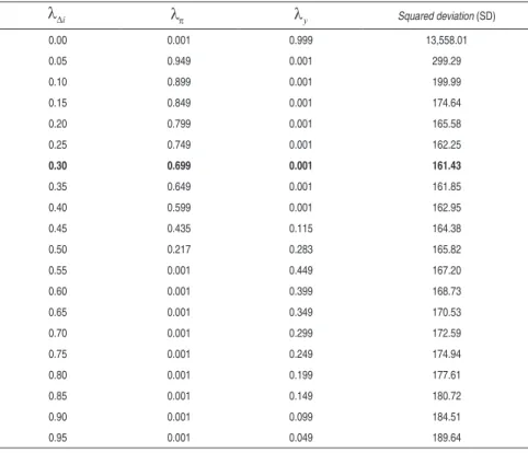
The calibrated parameters of the central bank’s loss function are
shown in Table 3, where the respective weights for andy which
result in smaller squared deviation (SD) correspond to each value
of i . Initially, a zero weight on interest rate smoothing produces a
very large squared deviation. This result evidences that the moneta-ry authority must have attributed a positive weight to interest rate smoothing in its loss function.
The results show that, when the central bank’s preference is incre-ased by interest rate smoothing, specifically from the interval 0.05 to 0.40, preference for inflation stability tends to grow, whereas preference for output stability tends to be mild or negligible (
y
=
0.00). The opposite is observed for weights on interest rate
smoo-thing greater than 0.50. For instance, for i=0.60, the weight for
inflation is virtually equal to 0.00, while the weight for the output gap is virtually equal to 0.40. Conversely, for interest rate smoothing weights greater than 0.80, the monetary authority is more concerned with the gradualist approach to the interest rate than with inflation and output stability around their targets.
Table 3 indicates that the parameters that minimize the squared deviation between the observed interest rate path and the optimal
interest rate are 0.699, y 0.001 and i 0.30. These results
reveal that the CRBP has adopted a flexible inflation targeting regi-me, placing a larger weight on inflation stability followed by interest rate smoothing and, finally, on output stability. These results are
23 The estimates obtained by SUR did not show large differences from those obtained by OLS
and did not change the calibration results. These results are available from the authors upon request.
24
For different discount factor (δ) values, there is no change in the identification of
relevant because they are consistent with the actions taken by the monetary authority during the current inflation targeting.
Table 3 - Central Bank’s Loss Function Estimated Parameters
i
y
Squared deviation (SD)
0.00 0.001 0.999 13,558.01
0.05 0.949 0.001 299.29
0.10 0.899 0.001 199.99
0.15 0.849 0.001 174.64
0.20 0.799 0.001 165.58
0.25 0.749 0.001 162.25
0.30 0.699 0.001 161.43
0.35 0.649 0.001 161.85
0.40 0.599 0.001 162.95
0.45 0.435 0.115 164.38
0.50 0.217 0.283 165.82
0.55 0.001 0.449 167.20
0.60 0.001 0.399 168.73
0.65 0.001 0.349 170.53
0.70 0.001 0.299 172.59
0.75 0.001 0.249 174.94
0.80 0.001 0.199 177.61
0.85 0.001 0.149 180.72
0.90 0.001 0.099 184.51
0.95 0.001 0.049 189.64
Source: Obtained from the authors.
Observe that the weight on output stabilization around its potential value is an interesting result. This may not have been an ultimate concern of the monetary authority in the inflation targeting regime (
y
= 0.001). Despite the low weight of output gap on the central
bank’s loss function, its insertion into the model is important as this variable is key to generating information on the behavior of future inflation (Dennis, 2006).
sustain economic agents’ inflation expectations (MEMORIA BCRP, 2002).
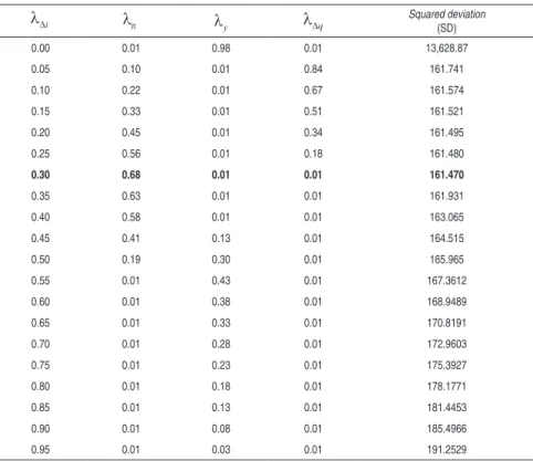
An interesting second exercise to be considered in the calibration process consists in knowing whether the CRBP has demonstrated any preference for nominal exchange rate smoothing, as in the study period, the Peruvian monetary authority made important
interven-tions in the exchange rate market.25 In addition, it also serves to
check whether the order of preferences of the monetary authority for inflation and output stability and interest rate smoothing re-mains robust to the inclusion of exchange rate smoothing in the loss function.
Table 4 - Central Bank’s Loss Function Estimated Parameters Including Preference for Exchange Rate Smoothing
i
y q
Squared deviation
(SD)
0.00 0.01 0.98 0.01 13,628.87
0.05 0.10 0.01 0.84 161.741
0.10 0.22 0.01 0.67 161.574
0.15 0.33 0.01 0.51 161.521
0.20 0.45 0.01 0.34 161.495
0.25 0.56 0.01 0.18 161.480
0.30 0.68 0.01 0.01 161.470
0.35 0.63 0.01 0.01 161.931
0.40 0.58 0.01 0.01 163.065
0.45 0.41 0.13 0.01 164.515
0.50 0.19 0.30 0.01 165.965
0.55 0.01 0.43 0.01 167.3612
0.60 0.01 0.38 0.01 168.9489
0.65 0.01 0.33 0.01 170.8191
0.70 0.01 0.28 0.01 172.9603
0.75 0.01 0.23 0.01 175.3927
0.80 0.01 0.18 0.01 178.1771
0.85 0.01 0.13 0.01 181.4453
0.90 0.01 0.08 0.01 185.4966
0.95 0.01 0.03 0.01 191.2529
Source: Obtained from the authors.
25
The results found for this second case are shown in Table 4 and re-veal that the order of preference for inflation and interest rate
smoo-thing has been maintained, with weights of 0.68 and i 0.30,
respectively. However, the preferences for exchange rate smoothing and output gap stabilization were non-significant, both with a weight equal to 0.01. These results suggest that: i) exchange rate smoothing has not played an important role in the CRBP’s loss function; ii) Exchange rate market interventions made by the Peruvian mone-tary authority were consistent with the current inflation targeting regime, precluding any conflict of objectives that could undermine the monetary authority’s credibility, which is absolutely necessary to sustain inflation expectations.
3.2.1 Optimal Monetary Policy Rule
According to the calibration strategy, the estimated parameters of the macroeconomic model and of the identification of preferences in the loss function imply that the optimal monetary rule, mentioned in Equation (20), is given by:
(30)
amounted to approximately 0.76. This result reflects the Peruvian monetary authority’s concern with interest rate smoothing.
The coefficients of the optimal monetary policy rule (30) repre-sent the immediate effect of explanatory variables on interest rates. Nevertheless, state variables also have secondary effects on the
inte-rest rate as a result of their lagged values and of the inertial term
i
t−1.These secondary effects can be measured by expressing the optimal monetary policy rule in the long run, given by:
i 1 2y3q4tt
0.595 1.199 0.225 0.346
i y q tt (31)
where
1 (f1 f2 f3 f4) / 1 f10
,
2 (f5f6) /
1f10
,
3 f7/ 1 f10
,
4 f9/ 1 f10
.
The results indicate that the long-term monetary rule responds strongly to the output gap, i.e., an increase of one percentage point in the output gap raises the interest rate by 1.199 percentage points, revealing a procyclical behavior towards the output gap. However, an increase of one percentage point in the inflation rate pushes the inte-rest rate up by 0.595 percentage points. The latter result shows that the Taylor (1993, 1998) principle is not satisfied. Notwithstanding, this result should be viewed with caution given that, in the case of a small open economy like that of Peru, other important variables in addition to output and inflation are taken into account in esta-blishing the monetary rule (such as terms of trade and exchange rate depreciation). Furthermore, these two variables are correlated with inflation, and through its indirect effects, they eventually influen-ce inflation rate movements. Therefore, not only can the effects of inflation on the interest rate be seen straightforwardly, that is, through contemporaneous inflation, but also indirectly through the terms of trade and exchange rate depreciation. On the other hand, similar results were obtained in other studies, as the ones conducted
3.2.2 Optimal Path versusObserved Interest Rate Path
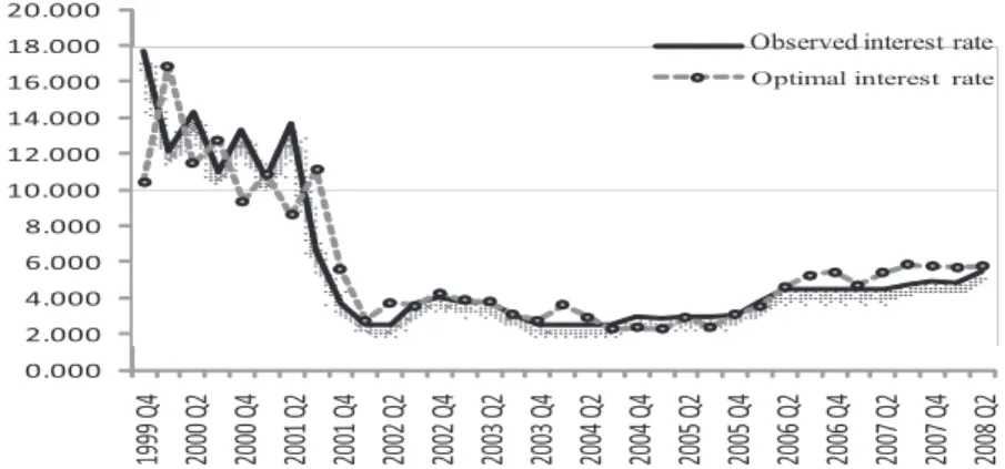
Figure 1 shows the path for the optimal interest rate associated with the preferences obtained by the calibration strategy and the
true interest rate path approximated by the interbank rate.26 Note
that the optimal interest rate captures the main movements of the observed interest rate. However, there are some inconsistencies, es-pecially in the first periods. For instance, the monetary authority with calibrated weights may have maintained the interest rate lower than the observed interest rate for the second and fourth quarters of year 2000 (period strongly influenced by uncertainty over the presidential elections) in response to lower expectations of exchange rate depreciation and inflation during that period.
On the other hand, the developments of the electoral year in 2000 exerted a strong impact on financial variables in 2001, chiefly du-ring the second half of 2001 when the interest rate went up from 11 to 14 percentage points. Nevertheless, Figure 1 shows that the monetary authority with an optimal behavior could have pushed the interest rate down to around 9 percentage points during the second quarter of 2001.
0.000 2.000 4.000 6.000 8.000 10.000 12.000 14.000 16.000 18.000 20.000
1999 Q4 2000 Q2 2000 Q4 2001 Q2 2001 Q4 2002 Q2 2002 Q4 2003 Q2 2003 Q4 2004 Q2 2004 Q4 2005 Q2 2005 Q4 2006 Q2 2006 Q4 2007 Q2 2007 Q4 2008 Q2 Observed interest rate Optimal interest rate
Figure 1 – Observed Interest Rate versus Optimal Interest Rate
Another important difference arises between the second half of 2001 to the first half of 2002, when the monetary authority could
26 This Figure shows the path for the optimal interest rate obtained by calibration without
have adopted an expansionary behavior to keep tabs on the marked deceleration of the inflation rate in that period. However, it is im-portant to note that the observed interest rate increased at a slower pace than did the interest rate predicted by the optimal rule asso-ciated with calibrated weights.
Finally, after 2002, the optimal path for the interest rate was very close to that of the observed interest rate. Despite that, some mi-nor inconsistencies can be encountered after the second quarter of 2006, when the optimal interest rate is above the observed interest rate, reaching a maximum difference of 104 basis points in the third quarter of 2007. This piece of evidence suggests that the monetary authority with an optimal behavior could have maintained a more contractionary monetary policy in order to overcome the adverse outcomes of the macroeconomic environment, brought about by the strong dynamism of domestic demand and of substantial increases in international prices (food and fuel), which ended up producing inflationary pressures.
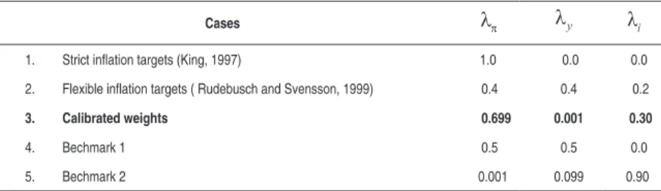
3.2.3 Comparison with Alternative Weights on the Loss Function
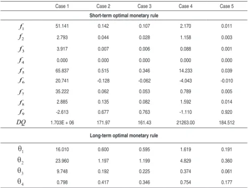
Another important analysis for the identification of central bank’s preferences includes the comparison of the optimal monetary policy rule derived from calibrated weights with monetary rules related to other weights. To do that, four different sets of weights were con-sidered, in addition to those obtained from the calibration process (see Table 5).
weight was used for interest rate smoothing and equal weights for the stabilization of inflation and output. The fifth case encompasses
combinations of
, y
which minimize the squared deviation of
the observed interest rate from the optimal interest rate for values
of i equal to 0.90.
27
Table 5 - Weights Used in the CRBP’s Loss Function
Cases
y
i
Strict inlation targets (King, 1997)
1. 1.0 0.0 0.0
Flexible inlation targets ( Rudebusch and Svensson, 1999)
2. 0.4 0.4 0.2
Calibrated weights
3. 0.699 0.001 0.30
Bechmark 1
4. 0.5 0.5 0.0
Bechmark 2
5. 0.001 0.099 0.90
Source: Obtained from the authors.
The respective optimal monetary rule was obtained for each set of alternative weights included in the central bank’s loss function. Thus, as shown in Table 6, in the cases in which a zero weight is used for interest rate smoothing (cases 1 and 4), the coefficients obtained for the optimal rules and the squared deviation had high values compared to those obtained by calibration (case 3). This result suggests that the Peruvian monetary authority used a positive weight for interest rate smoothing.
27 Dennis (2006) and Ozlale (2003) argued that optimal monetary rules provide better fit of
the interest rate path in backward-looking modelsif the monetary authority smooths the
Table 6 - Short-and Long-Term Optimal Monetary Rules for Different Weights on the CRBP’s Loss Function
Case 1 Case 2 Case 3 Case 4 Case 5
Short-term optimal monetary rule
1
f 51.141 0.142 0.107 2.170 0.011
2
f 2.793 0.044 0.028 1.158 0.003
3
f 3.917 0.007 0.006 0.088 0.001
4
f 0.000 0.000 0.000 0.000 0.000
5
f 65.837 0.515 0.346 14.233 0.039
6
f 20.741 -0.128 -0.062 -4.043 -0.010
7
f 35.222 0.062 0.053 0.789 0.005
8
f 2.885 0.135 0.082 1.592 0.014
9
f -2.613 0.677 0.763 -1.110 0.920
DQ 1.703E + 06 171.97 161.43 21263.00 184.512
Long-term optimal monetary rule
1
16.010 0.600 0.595 1.619 0.191
2
23.960 1.197 1.199 4.829 0.360
3
9.748 0.192 0.225 0.374 0.061
4
0.798 0.417 0.346 0.754 0.177
Source: Obtained from the authors.
For the set of weights corresponding to the flexible inflation target (case 2), the coefficients of the short- and long-term monetary policy rules had values very close to those found for the optimal moneta-ry rule derived from the calibration process. Notwithstanding, the squared deviation in case 2 was larger than in case 3. This suggests that the Peruvian monetary authority has come quite close to the application of the flexible inflation targets.
Case 1: Strict inflation target -450.000 -350.000 -250.000 -150.000 -50.000 50.000 150.000 250.000 350.000 450.000
1999 Q4 2000 Q2 2000 Q4 2001 Q2 2001 Q4 2002 Q2 2002 Q4 2003 Q2 2003 Q4 2004 Q2 2004 Q4 2005 Q2 2005 Q4 2006 Q2 2006 Q4 2007 Q2 2007 Q4 2008 Q2
Observed interest rate Optimal interest rate-KING
Case 2: Flexible inflation target
0.000 2.000 4.000 6.000 8.000 10.000 12.000 14.000 16.000 18.000 20.000
1999 Q4 2000 Q2 2000 Q4 2001 Q2 2001 Q4 2002 Q2 2002 Q4 2003 Q2 2003 Q4 2004 Q2 2004 Q4 2005 Q2 2005 Q4 2006 Q2 2006 Q4 2007 Q2 2007 Q4 2008 Q2
Observed interest rate Optimal interest rate Rudebush e Svensson
Case 3: Calibrated weights
0.000 2.000 4.000 6.000 8.000 10.000 12.000 14.000 16.000 18.000 20.000
1999 Q4 2000 Q2 2000 Q4 2001 Q2 2001 Q4 2002 Q2 2002 Q4 2003 Q2 2003 Q4 2004 Q2 2004 Q4 2005 Q2 2005 Q4 2006 Q2 2006 Q4 2007 Q2 2007 Q4 2008 Q2 Observed interest rate Optimal interest rate
Case 4: Benchmark 1
-50.000 -30.000 -10.000 10.000 30.000 50.000 70.000
1999 Q4 2000 Q2 2000 Q4 2001 Q2 2001 Q4 2002 Q2 2002 Q4 2003 Q2 2003 Q4 2004 Q2 2004 Q4 2005 Q2 2005 Q4 2006 Q2 2006 Q4 2007 Q2 2007 Q4 2008 Q2
Observed interest rate Optimal interest rate- BECHMARK-1
Case 5: Benchmark 2
0.000 2.000 4.000 6.000 8.000 10.000 12.000 14.000 16.000 18.000 20.000
1999 Q4 2000 Q2 2000 Q4 2001 Q2 2001 Q4 2002 Q2 2002 Q4 2003 Q2 2003 Q4 2004 Q2 2004 Q4 2005 Q2 2005 Q4 2006 Q2 2006 Q4 2007 Q2 2007 Q4 2008 Q2
Observed interest rate Optimal interest rate-BECHMARK2
Figure 2 - Observed Interest Rate versus Optimal Interest Rate
As shown in Figure 2, the optimal path for the strict inflation targets (case 1) and the path for the optimal monetary rule when a zero weight is used for inflation smoothing (case 4) exhibit large incon-sistencies relative to the true path for the interest rate, producing
positive and negative values with up to three digits.28 This
demons-trates that the Peruvian monetary authority has neither followed a strict inflation targeting regime nor used a zero weight for interest
28