Materials Research.
Anomalous Loss Hysteresis Loop
Adriano A. Almeidaa*, Daniel L. Rodrigues-Jra, Laura S. P. Perassaa,
Jeanete Leichtb, Fernando J. G. Landgrafa
aEscola Politécnica de Engenharia Metalúrgica e de Materiais, Universidade de São Paulo – USP,
CEP 05508-030, São Paulo, SP, Brasil bUniversity of Wales (Cardiff), United Kingdom
Received: July 1, 2013; Revised: January 16, 2014
This paper discusses the anomalous loss behavior in two electrical steels types. Starting from a non oriented electrical steel coil, three groups of samples with different grain sizes were produced. Grain oriented steel samples were produced from a commercially available material. The experimental procedure was performed by means of magnetic properties measurements using an Epstein frame. A procedure to draw the hysteresis curve of the anomalous loss is proposed. The results reported that anomalous loss has a different behavior when the two electrical steel types are compared. In non oriented steels anomalous loss is concentrated at the low induction region. In grain oriented steels, a remarkable participation of high induction region is observed.
Keywords: anomalous loss, hysteresis curve, non oriented steel, grain oriented steel
1. Introduction
One of the most important parameters for electrical steel selection is magnetic loss. This feature refers to the energy dissipated when the material is cyclically magnetized and demagnetized. Magnetic loss, or iron loss, is commonly divided in three parcels: hysteretic (or quasi static), classical eddy current (or parasitic) and anomalous loss (the term excess loss is often used too). This analysis method has been applied by the industry for decades1.
Microestructural characteristics affect the three parcels behavior. Other publications2-5 reported that features like grain size and texture have inluence over the hysteretic
and anomalous loss.
While hysteresis loss is calculated as the area of a experimentally measured hysteresis loop, allowing the discussion of energy dissipation mechanisms6-8 in different
areas of the curve, anomalous loss is obtained as the rest of a sum, giving no chance to such discussion. The present work proposes a procedure to draw the hysteresis of eddy current loss and, by geometrical differences, calculate and draw the hysteresis curve of anomalous loss. Applying these procedures to non oriented and grain oriented samples, energy dissipation mechanisms6-8 in anomalous loss are
discussed.
2. Experimental Procedure
In this paper two kinds of electrical steels were analyzed: grain oriented steel (GO) and non oriented steel (NO). The GO steel was produced by Aperam with thickness 0.27 mm, resistivity 49 µΩ.cm, density 7650 Kg/m3, grain size 3 mm
and chemical composition as described in Table 1. It was
made available in lat strips shape with dimensions 30 x 3 cm
and the rolling direction parallel to the length.
Non oriented electrical steel samples were extracted from a single coil, in annealed state, whose chemical composition is described in the Table 2. The initial thickness was 0.54 mm, density 7780 kg/m3, resistivity 25.67 µΩ.cm
and grain size 11 µm.
This material was cut, giving rise to strips for magnetic characterization with size 30 x 3 cm and length parallel to rolling direction. In order to produce sets of samples with different grain size a heat treatment was performed to provide grain size increasing by grain growth. The annealing parameters are described in Table 3.
The microstructural characterization was performed by means of micrographs extracted from a surface at mid thickness of the sample after metallographic preparation and chemical etching using Nital 3 %. The grain size measurement was performed using the intercept method in accord to ASTM standard9.
The analysis of the magnetic properties was made through a loss separation procedure, performed graphically. Therefore, hysteresis curves were produced corresponding to each of the portions that compose the total loss. Hysteresis loops related to total and hysteretic losses were directly obtained using an Epstein frame. In this equipment
the primary current was supplied by a power ampliier
KEPCO BOP50-80 with a waveform generator HP33120A/ dc-15 MHz. Sinusoidal induction with maximum value 1.5 T was used.
Total loss determination was measured by a wattmeter at frequency of 60 Hz for NO steel strips. For the GO steel samples tests at frequencies of 60 and 100 Hz were carried out. Hysteretic loss determination was made using
Almeida et al. Materials Research
a luxmeter Walker MF-3D connected to the Epstein frame
secondary coil and a shunt resistor connected to a multimeter HP 34401A, at 0.005Hz.
The eddy current loss calculation was carried out from the equation proposed by Bertotti10. The author describes a classical ield, Hcl, whose origin is due to induced parasitic currents. The classical field, Hcl, is determined using Equation 1.
( )
212
h cl
t dB H t
dt σ ×
= × (1)
where σ is conductivity, th is thickness and dB/dt is the variation rate of induction, B, as function of the time, t. Magnetic induction varies as a sinusoidal function of the time as reported by Equation 2 with Bm meaning maximum induction.
( )
m(
2)
B t =B ×cos π ×f t (2)
Thus, dB/dt can be derived from Equation 2 as described in Equation 3
m
dB
B 2 f sen(2 ft)
dt = − π π (3)
where f is the frequency.
Anomalous loss is treated here as a consequence
of an anomalous ield. Thus, it can be calculated in an
analogue way to the traditional method for anomalous loss determination11, in other words, by subtraction of magnetic ield values, at each induction level, as described
by Equation 4.
(
)
Bi Bi Bi Bi
anomalous total classical histeretic
H =H − H −H (4)
3. Results and Discussion
3.1.
Eddy current loss
Applying the equations previously presented in this paper one can note that the magnetic induction varies with
classic ield describing a closed ellipse as illustrated in
Figure 1.
Table 4 shows a comparison between the internal area of the B x Hcl loops described in Figure 1 and classical
Figure 1. B x Hcl loops for GO (A) and NO (B) samples for a magnetization cycle with maximum induction 1.5 T and frequency 60 Hz. Table 1. Chemical composition of the grain oriented electrical steel.
Si Al S C Nb Mn Cr Ti
3.22 0.0014 0.0297 0.0369 0.0022 0.0563 0.0138 0.001
Table 2. Chemical composition of the non oriented steel.
C Mn P S Si Cu Al Ni Cr Ti
24 ppm 0.5 0.016 0.0086 0.69 0.066 0.312 0.0108 0.025 0.001
Table 3. Annealing parameters and inal grain size of the non
oriented electrical steel samples.
A B C
Temperature (°C) 600 850 850
Time (hours) 2 4 8
Grain size after annealing (µm) 11 58 62
Table 4. Comparison between the internal area of the B x Hcl loops described in Figure 1 and classical eddy current loss estimated from Equation 5.
Pcl (J/m3)
GNO GO
Thomson - Equation 6 231.26 33.28
Anomalous Loss Hysteresis Loop
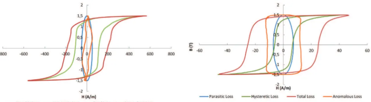
Figure 2. Loss separation for NO samples annealed for 2 hours at
600 °C with inal grain size 11 µm using peak induction 1.5 T and
frequency 60 Hz.
Figure 3. Loss separation for NO samples annealed for 4 hours at
850 °C with inal grain size 58 µm using peak induction 1.5 T and
frequency 60 Hz.
Figure 4. Loss separation for NO samples annealed for 8 hours at
850 °C with inal grain size 62 µm using peak induction 1.5 T and
frequency 60 Hz.
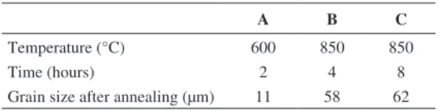
Figure 5. Loss separation for GO samples using peak induction 1.5 T and frequency 60 Hz.
Figure 6. Loss separation for GO samples using peak induction 1.5 T and frequency 100 Hz.
eddy current loss estimated from Equation 5, proposed by Thomson12, where B
m is maximum induction, ρ is resistivity
and d is density. These results indicate that both methods are equivalent for parasitic loss calculation.
( )² 6
m Cl
f B e P = π
ρ (5)
3.2.
Anomalous loss
Hysteresis loops for total loss and its parcels are illustrated in Figures 2, 3 and 4 for non oriented steels with grain size 11, 58 and 62 µm, respectively, and maximum induction 1.5 T.
The energy dissipation mechanisms in electrical steels are associated with displacement, nucleation and annihilation of domain walls6-8. According to Landgraf13,
along the low induction region (for induction ranging from –0.8 to 0.8 T) the main mechanism of energy dissipation is domain wall movement. The results for non oriented steel reveal that most of the anomalous loss activity takes place
in the low induction region and it is concentrated in the irst
and third quadrants. The excess loss decreases in the high induction region, where the magnetization by irreversible magnetic domains rotation prevails.
Figures 5 and 6 show the anomalous loss behavior for grain oriented samples. In opposition to the observed for non oriented steel, anomalous loss presents a remarkable participation at the high induction region. This different behavior can be associated with magnetic domain structure. In non oriented steels, that structure is complex due to the different grain orientations.On the other hand, in grain oriented sheets, one can use a model proposed by Pry and Bean14, which assume a periodic organization of magnetic
domains. Besides that, Shilling and Houze15 proposed the
existence of lancet domains. The annihilation and nucleation of these domains during the magnetization process have a great contribution for the anomalous loss increase as reported in16,17.
4. Conclusion
Almeida et al. Materials Research
steels are compared. In non oriented steels, anomalous loss is concentrated in the low induction region. On the other hand, in grain oriented samples, the results indicate remarkable participation of anomalous loss in high induction region. In
this case, there is inluence of the lancet domains nucleation/
annihilation phenomenon.
Acknowledgements
The authors thank Brasmetal Waelzholz SA, Aperam South America and Instituto de Pesquisas Tecnológicas - IPT.
Daniel L. Rodrigues-Jr and Adriano A. Almeida wish acknowledge the inancial support of CAPES.
References
1. Moses AJ. Electrical steels: past, present and future developments. IEE Procedings. 1990; 137(Pt. A 5). 2. Barros J, Schneider J, Verbeken K and Houbaert Y. On the
correlation between microstructure and magnetic losses in electrical steel. Journal of Magnetism and Magnetic Materials. 2008; 320:2490-2493. http://dx.doi.org/10.1016/j. jmmm.2008.04.056
3. CamposMF, Teixeira JC and Landgraf FJG. The optimum grain size for minimizing energy losses. Journal of Magnetism and Magnetic Materials. 2008; 301:94-99. http://dx.doi. org/10.1016/j.jmmm.2005.06.014
4. Rodrigues-Junior DL, Silveira JRF and Landgraf JGF.
Combining Mager and Steinmetz: The Effect of Grain Size and Maximum Induction on Hysteresis Energy Loss. IEEE Transactions on Magnetics. 2011; 47(9).
5. BertottiG. General properties of power losses in soft f e r r o m a g n e t i c m a t e r i a l s . I E E E Tr a n s a c t i o n s o n Magnetics. 1988; 24:624-630.
6. BoonCR and Robey JA. Effect of domain-wall motion on power loss in grain-oriented silicon-iron sheet. Proceedings of the Institution ofElectrical Engineers. 1968; 115:1535-1540. http://dx.doi.org/10.1049/piee.1968.0271
7. HallerTR and Kramer JJ. Model for Reverse-Domain Nucleation in Ferromagnetic Conductors. Journal of Applied Physics. 1970; 41:1036-1037. http://dx.doi. org/10.1063/1.1658805
8. GoodenoughJB. Summary of losses in magnetic materials.
IEEE Transactions on Magnetics. 2002; 38:3398-3408. http:// dx.doi.org/10.1109/TMAG.2002.802741
9. American Society for Testing and Materials - ASTM.
E 112 1996: Standard Test Methods for Determining Average
Grain Size. West Conshohocken: ASTM International; 2004.
10. BertottiG. Hysteresis in magnetism for physicists, Materials Scientists, and Engineers. Academic Press; 1998. p. 400-404. 11. CamposMF, Yonamine T, Fukuhara M, Landgraf FJG, Achete CA and Missell FP. Effect of Frequency on the Iron Losses of 0.5% and 1.5% Si Nonoriented Electrical Steels. IEEE Transactions on Magnetics. 2006; 42(10):2812-2814. http:// dx.doi.org/10.1109/TMAG.2006.879897
12. ThomsonJJ. On the heat produced by eddy currents in an iron plate exposed to an alternating magnetic.
Electrician. 1892; 28:599-600.
13. Landgraf FJG, Teixeira JC, Emura M, Campos MF and Muranaka CS. Separating components of the hysteresis loss of non-oriented electrical steels. Materials Science Forum. 1999; 302-303:440-445. http://dx.doi.org/10.4028/
www.scientiic.net/MSF.302-303.440
14. PryH and Bean CP. Calculation of the Energy Loss in Magnetic
Sheet Materials using a Domain Model. Journal of Applied
Physics. 1958: 29:532. http://dx.doi.org/10.1063/1.1723212 15. ShillingJW and Houze GL Jr. Magnetic properties and Domain
Structure in Grain-Oriented 3% Si-Fe. IEEETransactions on Magnetics. 1974; 10(2):195-223. http://dx.doi.org/10.1109/ TMAG.1974.1058317
16. ShillingJW, Morris WG, Osborn ML and Prakash R.
Orientation Dependence of Domain Wall Spacing and Losses
in 3-Percent Si-Fe Single Crystals. IEEETransactions on Magnetics. 1978; 14(3):104-111. http://dx.doi.org/10.1109/ TMAG.1978.1059739