WORKING PAPER SERIES
Universidade dos Açores Universidade da Madeira
CEEAplA WP No. 18/2011
Fuel Price Transmission Mechanisms in
Portugal
Francisco Silva Maria Graça Batista Nelson Elias
Fuel Price Transmission Mechanisms in Portugal
Francisco Silva
Universidade dos Açores (DEG e CEEAplA)
Maria Graça Batista
Universidade dos Açores (DEG e CEEAplA)
Nelson Elias
Universidade dos Açores (DEG)
Working Paper n.º 18/2011
Julho de 2011
RESUMO/ABSTRACT
Fuel Price Transmission Mechanisms in Portugal
This study aims to analyze the behavior of fuel prices at the pump (unleaded gasoline and diesel) in Portugal, relative to positive and negative variations in Brent Crude Oil prices. Applying an autoregressive distributed lags model (ARDL) to weekly time series data for the period of January 2004 through May 2009, we detected some signs of asymmetry in the transmission price mechanism. However, these patterns are not statistically significant enough to reject hypotheses of symmetry in the price adjustment mechanisms of fuels in Portugal.
Keywords: fuel and oil prices, price adjustment mechanisms.
Francisco Silva
Universidade dos Açores
Departamento de Economia e Gestão Rua da Mãe de Deus, 58
9501-801 Ponta Delgada Maria Graça Batista Universidade dos Açores
Departamento de Economia e Gestão Rua da Mãe de Deus, 58
9501-801 Ponta Delgada Nelson Elias
Universidade dos Açores
Departamento de Economia e Gestão Rua da Mãe de Deus, 58
FUEL PRICE TRANSMISSION MECHANISMS IN PORTUGAL
FRANCISCO SILVA
Departamento de Economia e Gestão Universidade dos Açores
CEEAplA Apartado 1422
9501-801 Ponta Delgada, Azores; Portugal Tel.: 296 650 084
Fax: 296 650 083 fsilva@uac.pt
MARIA DA GRAÇA BATISTA Departamento de Economia e Gestão
Universidade dos Açores CEEAplA
Apartado 1422
9501-801 Ponta Delgada, Azores; Portugal Tel.: 296 650 084
Fax: 296 650 083 mbatista@uac.pt
NELSON ELIAS
Departamento de Economia e Gestão Universidade dos Açores
Apartado 1422
9501-801 Ponta Delgada, Azores; Portugal Tel.: 296 650 084
Fax: 296 650 083 nelsonelias2010@hotmail.com
FUEL PRICE TRANSMISSION MECHANISMS IN PORTUGAL
ABSTRACT
This study aims to analyze the behavior of fuel prices at the pump (unleaded gasoline and diesel) in Portugal, relative to positive and negative variations in Brent Crude Oil prices. Applying an autoregressive distributed lags model (ARDL) to weekly time series data for the period of January 2004 through May 2009, we detected some signs of asymmetry in the transmission price mechanism. However, these patterns are not statistically significant enough to reject hypotheses of symmetry in the price adjustment mechanisms of fuels in Portugal.
INTRODUCTION
The general view of consumers is that final fuel prices increase at a higher and faster rate when the price of crude oil increases. In turn, they decrease at a slower rate when the price of crude oil decreases. In other words, these prices point to the presence of asymmetry in this transmission mechanism. This perception is supported by many organizations which, in defense of consumer interests, criticize the functioning of the market, namely the pricing policies of companies involved and how governments regulate them.
The main purpose of this study is to analyze fuel prices (unleaded gasoline and diesel) and their relationships to oil prices in international markets. In other words, this study will verify if the price variations between gasoline stations is consistent, or not, considering the changes in the prices of oil. If this price transmission mechanism of oil to fuel is not consistent in its variations, it means the process is asymmetric.
Since the works of Bacon (1991) and Manning (1991), the topic of adjustment of downstream prices relative to upstream ones has been well studied in many markets. The countries which have a greater incidence of analysis include the United States and United Kingdom, followed by other European countries, namely France, Italy, Germany and Spain. Despite this being a widely studied subject internationally, there is only one study of this kind in Portugal, by the Autoridade da Concorrência (the Portuguese competition authority; 2008), hereafter referred to as the AdC. Hence, this study will contribute to the literature on this topic in relation to the expansion of the existence of limited knowledge of issues related to the adjustment of fuel prices in Portugal.
The inefficiency in the pricing system derived from the aforementioned contingent asymmetries may affect companies and individuals with increases in transportation and production costs, decreases in purchasing power, and increases in inflationary pressure.
This leads to the perception that the market is not functioning efficiently, as there is great interest in researching this phenomenon.
The rest of this paper is structured as follows. The paper begins with a revision of the main literature on the subject of fuel price adjustment. It continues with the presentation of the methodology, data that were used and the results of the analysis. The final section includes the conclusions and implications of this research investigation.
LITERATURE REVIEW
The system of adjustment of downstream prices in relation to upstream ones is a point of interest, not only in the fuel market, but also for other goods, such as agricultural foods (e.g., vegetables, meat, and wheat) and financial (e.g., interest rates and bank deposits) products.
Abdulai (2000) studied the reflection on the price relationships in the primary corn markets of Ghana. Abdulai (2002) analyzed the Swiss market in terms of adjustments between retail and wholesale pork prices. Still on the topic of agricultural products, Gomez et al. (2010) analyzed asymmetry in the transmission of coffee prices in France. Mohanty et al. (1995), on the other hand, analyzed the adjustment mechanisms of wheat prices in international markets. The results of most of the previous studies point to asymmetric patterns in the transmission of prices, with a rise in the producer price being transmitted more rapidly to the final price, then when there is a decline.
One of the pioneers in relation to addressing this issue for the oil and fuel market was Bacon (1986), who dubbed the term “Rockets and Feathers” (Bacon, 1991), illustrating the effect that the final cost of gasoline suffered from variations in the costs from when it left the refinery. The term now known in this scope imply that the final prices of gasoline rise as rockets in response to increases in the oil costs, but fall like feathers when the price of oil goes down. This author analyzed the United Kingdom
(UK) gasoline market with a Quadratic, Partial Adjustment Model using biweekly data from 1982 to 1989. He noticed the adjustments of gasoline prices at the pump showed a faster increase than decreases at the refinery.
In the cases of variations in exchange rates, Bacon (1986) confirmed an additional delay of two weeks for it to be applied to the final gasoline prices. The term “quadratic” used by this author was indicated as a limitation (Borenstein et al., 1997), due to making the asymmetry seem proportionally greater, according to the difference between retail prices and a long-term equilibrium price increase.
With an ARDL model, Karrenbrock (1991) analyzed the United States (USA) market for the 1983-1990 period, finding patterns of asymmetry in the time it took for retail gasoline prices to respond to variations in the price at the refinery. This model of linear adjustment allows for the testing of several hypotheses of asymmetric patterns related to the adjustment of prices: the present-day, accumulated and period-to-period effects. This author concluded that 69% in the increase of the average, wholesale gasoline price is passed onto the consumer during the first month. Consequently, when the cost lowers, an adjustment from 22% to 32% occurs. According to Karrenbrock (1991), the main reason for such an asymmetry is the concentrated industry. Like Bacon (1991), he also concluded that the adjustment is reflected in the final prices after approximately two months.
Shin (1994) studied refinery gasoline prices in relation to monthly oil prices in the USA throughout the 1986-1992 period. He used a Partial Adjustment Model (PAM) model, similar to the one used by Bacon (1991). However, Shin (1994) did not reject the hypothesis of symmetry in the adjustment of prices in the first phase (oil-refinery) and the second phase (refinery-retail) test was inconclusive.
Salas (2002) stands out from the others by using three different models to analyze the gasoline price adjustments in the Philippines between 1999 and 2002. Shin deals with the issue of price deregulation, which occurred in 1998. Through market power analysis, the companies were separated in two groups: large and small companies. The Ordered Probit model is used to determine that eight weeks constitutes the most adequate number of lag periods to use in the other two models. Through the PAM and ECM models, this author detected asymmetric patterns in the adjustment of prices and that the reaction of the companies to price management varies according to the size of the company. Results show that large companies passed on variations of oil and retail prices more rapidly than small ones. A situation considered less consistent in this author’s study is related to the cumulative function of price adjustments, calculated with non-significant coefficients.
More recently, Adilov and Samavati (2009) used an ARDL model with similarities to the model by Karrenbrock (1991). They focused their study on the USA market, analyzing nine states individually during the 1991-2007 period. They tried to overcome one of the limitations of Borenstein et al. (1997), concerning the type of data used, pointing out the use of average prices in certain cities to make a national analysis which could lead to biased results.
Manning (1991) differed himself substantially from the others, except for Salas (2002), in relation to the econometric model used, being a pioneer in the use of the error correction mechanism (ECM) for an analysis of fuel price adjustments. This author focused his study on the UK market with monthly data on gasoline during the period of 1973 to 1988, detecting some patterns of asymmetry in the prices of gasoline in relation to the prices of oil. However, these asymmetric patterns were of little significance and of short duration. It was concluded that the final price adjustments of
gasoline in relation to a variation of the oil price, occurred within four months, longer than the period observed by Karrenbrock (1991). This author tests the stationarity and cointegration of a series of data, an essential procedure when using the ECM model.
Kirchgässner and Kübler (1992) focused their study on the German (Western Germany) market with monthly data from the period of 1972 to 1989. These authors studied the response of gasoline prices in relation to spot prices in the Rotterdam market, subdividing the analysis into two periods: before and after January 1989. Like Manning (1991), they employed an ECM model, which detected differences of adjustments in the 1972-1980 period, whereas they could not reject the hypothesis of symmetry in the adjustment of prices after 1980. By their study, the reactions of long-term prices did not present significant differences between the two periods. It should be stressed that, contrary to the majority, this study detects a transmission of prices faster on the descent than on the ascent.
Borenstein et al. (1997) also used an ECM model, with some modifications related to Manning (1991) and Kirchgässner and Kübler (1992), to test asymmetry in the transmission of fuel prices in each of the distribution and production phases from the oil, refinery, and wholesale distributor price to the final cost. This was done through weekly data from 1986 to 1992 in the USA market.
These authors reached the conclusion that asymmetry exists in the price adjustments of all of the phases under study, while the downstream prices reacted more rapidly to rises than drops of upstream prices. They presented three possible interpretations for the existence of the asymmetric behavior of prices: (I) oligopoly of sellers, (II) times of production and inventories and, (III) volatility in oil prices in relation to competition in the retail market.
Eltony (1998) and Reilly and Witt (1998) used monthly data on gasoline prices in the UK and USA to apply a ECM model similar to the one in Manning (1991), with relative modifications to the model in Borentein et al. (1997). These two studies are very similar, differing only during the period of analysis and inclusion by Eltony (1998) of the UK analysis. The hypothesis of symmetry in the final price of gasoline in response to the ups and downs of oil prices is rejected. In the same manner, the hypothesis of symmetry in response to the exchange rate in the adjustments of gas prices is rejected.
Upon attempting to overcome a limitation from the previous studies of individual countries and regions, Galeotti et al. (2003) present a more ample study with an analysis of five European countries (France, Spain, Italy, Germany and the UK) using monthly data from the 1985-2000 period. These authors based their analysis on three phases of the oil industry’s distribution chain to determine possible differences, whether they are in the refinery stage, the distribution phase or both. An asymmetrical ECM model is used to distinguish short-term asymmetric patterns from the long-term adjustment periods and test the effect of exchange rates in the transmission mechanism of prices.
The results point to signs of imbalance in both short-term and long-term adjustments. In line with Bacon (1991), Reilly and Witt (1998), and Eltony (1998), the exchange rates are included in this mechanism. The effects of the exchange rates are statistically significant and conclude that gasoline prices respond more rapidly to rises than falls of dollar/Euro exchanges. The calculation of adjustment periods in the final prices to variations of downstream prices is also considered. Furthermore, Galeotti et al. (2003) calculated the number of weeks needed to reach 50% and 95% of the deviation between the current price and the balanced price. Some differences were detected
between the countries and phases studied. The oil–retail phase detects greater asymmetry in the price adjustment periods in France, Germany and the UK.
Based on the model used by Borenstein et al. (1997), the AdC (2008) analyzed the system of market fuel prices in the European Union with the 15 member states during the 2004-2008 period. Cumulative response functions were calculated in relation to each investigated phase (oil-refinery, refinery-PMAI or oil-PMAI - Average prices before taxes).
The AdC detected the existence of asymmetry in the case of diesel in the oil-refinery phase and in both forms of fuel in relation to the oil-refinery-retail phase in some member states. The former two were integrated into one single phase, namely oil-retail, concluding that it only increased the asymmetry patterns in regards to diesel and dropped slightly in regards to gasoline. In Portugal, prices tended to be completely adjusted to the variations of refinery prices, with a lag of four to five weeks in diesel prices and five to six weeks in gasoline prices. Although some signs of asymmetry were detected, the AdC states that the workings of the liquid fuel market in Portugal are very similar to the general market in the other countries of the European Union, rejecting the hypothesis of competition law violations by the market companies.
From the literature review, we observe the attempts of certain authors to identify the factors that cause these asymmetric patterns. Brown and Yucel (2000) name market structure, accounting methods, research costs, stock policies and consumer response as the primary cause of price shifts, without actually proving this. Kaufmann and Laskowski (2005) concluded from an econometric analysis of monthly USA data that the asymmetric relationship between oil and gasoline prices stems from the refining costs and the company’s inventory process. Borenstein et al. (1997) presents three possible explanations for the phenomenon: (I) the companies tend to keep prices high
after a drop in upstream costs, because they do not see changes in demand. The consumers, in general, do not immediately realize the variations in these costs, allowing the same demand with greater margins for the sellers. When demand starts to drop, the companies lower prices accordingly. (II) On the other hand, an occasional excess in demand makes the prices rise rapidly, due to unlimited stocks and production delays (production is unable to adjust itself immediately). However, an excess in supply causes the prices to drop more slowly, due to the limited stocks and lags in production. This is the case since there is not a current excess of products, only an amount expected for the existing demand. (III) Finally, these authors state that in periods of greater volatility in fuel prices, there is less demand when consumers observe changes in the price, implying that these variations reflect a change in costs, instead of altering the sellers’ margins. This may allow the companies to pass on the selling prices more rapidly, invoke an increase in costs (oil or refinery), and in the case of a decrease, the companies may delay that passing for the selling price. Several authors have launched hypothetical reasons for the causes of this asymmetric behavior in the fuel market without being able to sustain their claims.
We can point out a significant interest in researching this theme by the variety of existing literature. However, this subject is still poorly studied in Portugal, despite its relevance. One reason this subject should be a point of interest is the sheer national reliance on this form of energy. Another reason is the great impact on the price variations on the economic agents.
In the literature, the methodology used is quite varied. The most commonly used model is the ECM with its various forms. Regarding products, gasoline is the most studied fuel, whereas only Johnson (2002) and AdC (2008) appear to be the exceptions, with the inclusion of the price analysis of diesel. The periodicity of the data is largely
monthly or weekly and the obtained results do not vary significantly between schedules (Frey and Manera, 2007).
By including both types of fuel and relative data for a recent time period, this study makes it possible to compare the behavior of price transmission for both gasoline and diesel with the intention of furthering research on the subject in Portugal.
THE MODEL
After researching some of the econometric models used in literature on the subject, the ARDL model was chosen for an in-depth study. This decision is closely followed by the methodology of Karrenbrock (1991) and Adilov and Samavati (2009).
First to be tested was the long-term relationship between fuel prices (unleaded 95 octane gasoline and motor diesel separately) and the oil price, in which the former are dependant variables and the latter is an independent one. The relationship of this causality between the retail prices of oil and fuel was broached by Rao (2007), who concluded that there is a stable long-term relationship between these variables. As suggested by the economic theory, he concluded that the final fuel prices are greatly dependant on the oil prices. This relationship can be seen in the following equation:
C α α p ε (1)
Assuming the adjustment takes (k) periods to occur, the total adjustment of the fuel prices to an initial variant in the oil price (∆P , can be provided as follows:
∆C β ∆P β ∆P β ∆P ∑ β∆P (2) C represents the price to be analyzed (gasoline or diesel), while ∆ is the operator of the first difference. This equation assumes there is a symmetric response in relation to the rise and fall in the price of oil. We present the variation of prices in each period as ∆C C C and ∆P P P , respectively.
To incorporate an asymmetric response, we classify β with the signs (+) e (−), according to positive and negative variations in the oil price, respectively. This classification is given by the following rule:
∆C ∆C D with ∆C 0
∆C ∆C D with ∆C 0
∆P ∆P D with ∆P 0 ∆P ∆P D with ∆P 0
Where: D is a binary variable that receives the value of one when the expressions ∆C and ∆P are greater than zero, becoming zero otherwise. Therefore, the following dynamic model was tested for each type of fuel:
∆C α ∑ β ∆P β ∆P γT ε (3) The coefficients β represents fuel price adjustments for each period in relation to positive or negative variations in the oil price, according to the (+) or (−) signs respectively. The variable T was added to the model to capture a possible trend, while
represents the residual regressions, assuming white noise (for all of t) with a zero-mean average, as well as constant and uncorrelated variation with the independent variables. This model gives the effect of fuel price adjustments in each period, resulting from a rise or drop in the prices of oil.
The number of lag time weeks included in the regression is given by K=6 and the weighting results between the number of periods used by the other authors and by the test data. The analyzed literature and data gathering procedure made it possible to obtain results in which six weeks of lag gave satisfactory test results of the coefficients. We then made sure whether the results could be influenced by the lag periods; the primary conclusions were unchanged with the inclusion of more or less periods.
Variations in the price of Fuel
Kirchgässner and Kübler (1992) and Asplund et al. (2000) consider two monthly lags. Borenstein et al. (1997) and Salas (2002) use an eight-week lag, while Lewis (2005) includes a four-week delay. The TCA (2008) accounts for five weeks. The use of a lag longer than six weeks for testing the model seems to be inadequate, considering that the effect is less and statistically insignificant from the fourth week onwards.
The accumulated effect in response to fuel prices for each period k, given by ∑ β or ∑ β , can be calculated by the summation of the adjustment occurrence since moment zero (the moment of variation of oil prices) up to and including period k. In this study, the number of periods varies from 0 to 6, taking into account a lag of up to six periods in testing the econometric model. The effect accumulated in the final prices is calculated for the cases of positive or negative variations in the oil price as follows:
Positive Accumulated Effect β … β = ∑ β (4) Negative Accumulated Effect β … β = ∑ β (5)
The aforementioned methodology makes it possible to formulate and test the hypotheses related to the adjustment behavior of the fuel prices. The comparison of the positive coefficients β with the negative β ones and their individual significance makes it possible to analyze the symmetry for each period. This particular hypothesis formulation is as follows:
H : β β Symmetry H : β β Asymmetry
There is symmetry in this process when the upstream adjustment of the final price of fuels to positive and negative variations in the oil price is statistically identical. This occurs when it is impossible to reject H .
The accumulated adjustment effect can be analyzed by the formulation of the null hypothesis, when the summation of the βetas is equal after a positive and negative variation, in reference to oil priced. To this end, the accumulated positive and negative effect is calculated, respectively, by the statistically acceptable summation of β and β .
H : β β
Accumulated equal adjustments in the positive and negative variations
H : β β
Accumulated differing adjustments in the positive and negative variations
s and d may vary between 0 and 6, taking the statistical significance into account. There is symmetry (asymmetry) when the accumulated effect of the fuel prices is equal (different) in relation to the increase or decrease of the oil price.
We can even make this analysis in terms of verifying the possibility of a single adjustment, when all variations of the upstream price are passed onto the downstream price. If it is lower than 1, it is called partial, and if it is higher, it is called the “overshooting” effect.
STATIONARITY AND COINTEGRATION
If the series data considered are stationary, then the ARDL and ECM models may be consistently tested through the MMQ. Otherwise, if they are not as noted by Granger and Newbold (1974) the linear regression analysis may provide biased results (Frey and Manera, 2007). Therefore, verifying the variables that allows for an authentic long-term relationship requires the testing of their stationarity and cointegration (Engle and
Granger, 1987 and Stock, 1987). In the case of the calculations of ECM models, it is essential that the variables are cointegrated.
The economic variables are generally integrated in the 1st order, implicating the need of differentiating them once to make them stationary. In short, a variable is stationary when the joint probability distribution remains stable over time. This is assuming that the future will be consistent with the past, i.e., we can predict the future based on the past information. On the other hand, cointegration is a statistical property that guarantees the existence of a long-term genuine relationship between the series (Engle and Granger, 1987).
The first test involved the stationarity of the series of prices of fuels, oil and exchange rates. For that purpose, the following OLS (ordinary least squares) equation was formulated:
∆Y α δ Y ∑ β ∆Y U (6)
Y represents the variable to be tested, differentiated ∆Y and with lag Y , while U is the random residual term. The approach of the Dickey-Fuller (ADF) method was used to test the hypothesis that Yt is integrated in order 1. In other words, it has a
unitary root:
H : δ 0 Not Stationary H : δ 0 Stationary
The statistic Student’s t-distribution value associated with the test coefficient δ is compared to the critical value provided by the tables with the ADF test values (Dickey and Fuller, 1979). If the statistical t, in its absolute value, becomes superior to the critical value in the tables, the null hypothesis that indicates a non-stationarity of the variable is discarded. Coefficients were calculated for the four series, in Euros/liters, except for the exchange rate presented in USA dollars / Euros, fixed as K = 6 (Table 1).
According to the results in Table 1, we can infer that all variables are non-stationary since the statistical values cannot reject H : δ = 0 to a level of significance of 1%, relative to the critical value of -3.42. The values of δ reinforce this conclusion, since they all present values very close to zero in each series.
Table 1. Results of the stationarity tests.
Variable t Critical t 1%
Petroleum €/lt -0,021 -2,383 -3,42 Unleaded Gasoline €/lt -0,012 -2,327 -3,42
Diesel €/lt -0,008 -2.138 -3,42
Dollar/euro Exchange rate -0,015 -1,594 -3,42
The stationarity of the first differences made use of a similar formula to the previous one (6), except with terms differentiated once, resulting in the following:
∆∆Y α δ ∆Y ∑ β ∆∆Y U (7)
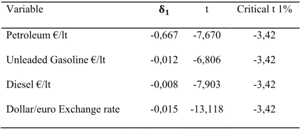
The statistical values presented in Table 2 make it possible to reject the same null hypothesis of non-stationarity for all variables. Therefore, it is assumed, in this analysis, that the variables are of first-order stationarity.
Table 2. Results of stationarity tests for the first differences.
Variable t Critical t 1%
Petroleum €/lt -0,667 -7,670 -3,42 Unleaded Gasoline €/lt -0,012 -6,806 -3,42
Diesel €/lt -0,008 -7,903 -3,42
When the variables are integrated in the same order, they meet one of the requirements for cointegration. This is precisely the next step of the research.
The method proposed by Engle and Granger (1987) was used to test the cointegration between the dependant variables (unleaded and diesel) and the independent ones (oil and exchange rates). First, the following OLS equation representing the cointegration or long-term relationship between the variables to be tested is calculated:
Y α β X (8)
The next phase consists of the residual analysis, resulting from the long-term relationship Y α β X . For each fuel type, the residual data is tested based on their stationarity, as in the following relationship:
∆ δ δ ∆ ∑ θ ∆ v (9)
The same number of lag periods from the stationarity test is used, meaning six weeks. With the calculation of coefficient δ , we can test the following hypotheses:
H : δ 0 Non Stationary Residuals H : δ 0 Stationary Residuals
The residual stationarity analysis makes it possible to infer whether both series are cointegrated or not. If the residuals of the relationship between both are stationary (rejection of H ), it is assumed the variables are cointegrated.
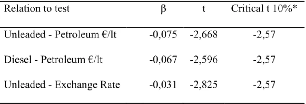
Table 3. Results of cointegration tests.
Relation to test β t Critical t 10%*
Unleaded - Petroleum €/lt -0,075 -2,668 -2,57 Diesel - Petroleum €/lt -0,067 -2,596 -2,57 Unleaded - Exchange Rate -0,031 -2,825 -2,57
Diesel - Exchange Rate -0,035 -2,841 -2,57
For the Table 3 values, resulting from the calculation of equation (9), the null hypothesis of non-stationarity of the residuals is rejected with a significance level of 10%. In other words, we can assume the existence of a long-term relationship between the prices of fuels and oil, a fact consistent with the majority of results obtained by other studies on the subject. For the relationship of the two fuel types and the exchange rate, the conclusion is the same, due to the rejection of the hypothesis of non-stationarity in the residuals of the long-term relationships (8) between these variables.
A sensibility analysis was made for the cointegration test, which detected a slight increase in the value calculated by the t-distribution with a reduction of the lag periods used in expression (9), making it possible to reject the same hypothesis to a significance level of 5% in most cases, with K< 6.
Based on these results and the economic theory, it is assumed that these are first-order stationarity variables cointegrated between themselves. When the variables are cointegrated, the calculators of equation (8) are consistent and asymptotically efficient (Stock, 1987) and the best specifications of the short and long-term relationships made through the error correction model (Engle and Granger, 1987).
DATA
The estimation of the empirical models was used for a series of weekly (minimum periodicity available for the fuel prices in Portugal) oil prices, the final costs of diesel and unleaded gasoline and the exchange rate between 01-02-2004 and 05-08-2009, representing a sample of 280 weeks. The use of a weekly periodicity seems reasonable, considering its frequent use in researching the matter. After monthly periodicity, weekly data is the second most commonly used data in the literature (Frey and Manera, 2007).
The price of Brent oil (Weekly Europe Brent Spot Price FOB) was quoted in London. A reference for the prices in Western Europe was obtained from the Energy
Information Administration website in dollars/ barrel. It was necessary to convert the
values to Euros/ liter, dividing the series into the base value of 158.76 liters, the equivalent of one barrel, according to the dollar/Euro exchange rate for the average of the respective week.
The weekly prices of 95 octane gasoline and motor diesel were obtained from the website of the Direcção Geral de Energia e Geologia (the Portuguese general institution of energy and geology, at: http://www.dgeg.pt/). Although there were available prices for other fuel types, unleaded 95 octane gasoline and motor diesel represent most of the consumption in Portugal. According to 2008 data, gasoline and diesel represent roughly 48% (11% gasoline and 37% diesel) of the total consumption of road fuel, according to the Portuguese competition authority (AdC, 3rd and 4th quarters of 2008).
The exchange rate was obtained from the European Central Bank website (http://sdw.ecb.europa.eu/), originally published daily with the USA dollar value for each Euro. Since the frequency of the periods used is daily, it was necessary to convert them to weekly to calculate the average daily exchange rate. To compensate for the lack of values for certain dates (e.g., holidays), those were filled in by the values of the day before.
EMPIRICAL RESULTS
The calculations from the empirical model (ARDL, given by expression 9) were made through the OLS in the statistics computer program SPSS and resulted in the following table:
Gasoline Diesel Parameters Coeficients p-value Coeficients p-value
0,000 0,784 0,001 0,491 -0,044 0,661 -0,014 0,857 0,376* 0,00 0,472* 0,000 0,454* 0,000 0,569* 0,000 0,190*** 0,058 0,171** 0,030 0,133 0,182 0,149*** 0,058 0,134 0,185 0,045 0,565 0,140 0,167 0,012 0,884 0,000 0,715 0,000 0,083 0,044 0,655 0,082 0,291 0,504* 0,000 0,367* 0,000 0,465* 0,000 0,268* 0,001 0,202** 0,042 0,168** 0,031 0,073 0,468 0,058 0,462 -0,028 0,783 0,034 0,667 0,009 0,929 0,104 0,182 . 0,49 - 0,58 - 280 - 280 - 1,59 - 1,22 - 18,25 0,000 25,79 0,000 * significant at 1%; ** significant at 5%; *** significant at 10%.
From the analysis of calculated coefficients with variables in levels, we succeeded in capturing a variation, in monetary units, suffered by the final fuel price in relation to a unitary variation in the oil price.
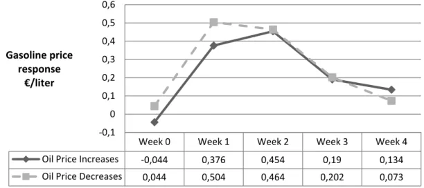
In line with the previous calculations, the results point to an adjustment that primarily occurs three to four weeks after the variation in oil price. In the same manner, the immediate effect (week 0) of the fuel prices to a positive or negative variation in the oil prices is small and statistically insignificant for both fuel types. In relation to model adjustment, there is a higher value in the case of motor diesel, with an adjusted of 0.58 compared to 0.49 for 95 octane gasoline. The constant (α) and coefficient (γ) associated with the trend variable is not statistically different from zero for both fuel types, meaning an insignificant influence on this model of a price adjustment. Figure 1 helps illustrate a more significant effect on the gasoline price during the first week, presenting a slight difference between the increase and decrease in the oil price.
Figure 1. Effect on gasoline price of variations in the oil price.
For example, when the oil price goes above €0.1/liter, the gasoline price rises to €0.038/liter in the first week, while a decrease of €0.1/liter in oil leads to a decrease of €0.05/liter in the gasoline price during the same period. In the second and third weeks following a change in the oil price, the increase and decrease in the gasoline price are
Week 0 Week 1 Week 2 Week 3 Week 4 Oil Price Increases ‐0,044 0,376 0,454 0,19 0,134 Oil Price Decreases 0,044 0,504 0,464 0,202 0,073 ‐0,1 0 0,1 0,2 0,3 0,4 0,5 0,6 Gasoline price response €/liter
relatively similar, registering approximate values of €0.046/liter and €0.02/liter, respectively. The fourth week shows a slight difference, with greater increases than decreases.
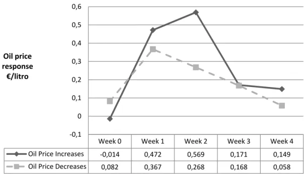
The results are slightly different for motor diesel, especially in the second week, after an initial variation in the oil price. As seen in Figure 2, there is a greater effect during the first and second weeks of an increase in the oil price, compared to a decrease in the latter. The behavior in the third and fourth weeks is similar to the increase and decrease of the upstream.
Figure 2. Effect on diesel price of variations in the oil price.
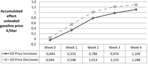
The analysis of the effect of the accumulated adjustment of fuel prices k weeks after a positive/negative variation in the oil price makes it possible to verify some of the differences in this price adjustment mechanism. For gasoline, as seen in Figure 3, there is a greater accumulated effect in response to a negative initial variation in the oil price.
Figure 3. Accumulated adjustment effect on the gasoline price.
Week 0 Week 1 Week 2 Week 3 Week 4 Oil Price Increases ‐0,014 0,472 0,569 0,171 0,149 Oil Price Decreases 0,082 0,367 0,268 0,168 0,058 ‐0,1 0 0,1 0,2 0,3 0,4 0,5 0,6 Oil price response €/litro
The opposite occurs in the case of diesel, demonstrating a greater response when the oil price increases. In the fourth week, Figure 4 shows that an initial increase of €0.1/liter in the oil price makes the diesel price increase by around €0.0135/liter. A decrease of €0.1/liter in the oil price causes a decrease of €0.095/liter in the diesel price after four weeks.
Figure 4. Accumulated adjustment effect on the diesel price.
This adjustment makes it possible to verify that the accumulated effect points to the existence of a complete transmission that is slightly superior to the oil price to fuel price. This is usually shown in research of this subject, with several studies pointing to
Week 0 Week 1 Week 2 Week 3 Week 4 Oil Price Increases ‐0,044 0,332 0,786 0,976 1,109 Oil Price Decreases 0,044 0,548 1,013 1,215 1,288 ‐0,2 0 0,2 0,4 0,6 0,8 1 1,2 1,4 Accumulated effect unleaded gasoline price €/liter
Week 0 Week 1 Week 2 Week 3 Week 4 Oil Price Increases ‐0,014 0,458 1,027 1,198 1,347 Oil Price Decreases 0,082 0,449 0,717 0,885 0,943 ‐0,2 0 0,2 0,4 0,6 0,8 1 1,2 1,4 1,6 Accumulated effect diesel price €/liter
full transmission of the upstream prices to the downstream prices. The results of Bacon (1991) and Karrenbrock (1991) also point to this situation, while Borenstein et al. (1997) presents values close to 0.8.
From a general analysis standpoint, we highlight the differences detected in the adjustment effect of the final prices for gasoline and diesel. In the case of gasoline, there is a greater proportional adjustment in decreases, than in increases, of the downstream price. On the other hand, diesel suffers a greater effect from increases in the oil price, showing greater evidence of asymmetry than in the case of gasoline, in which the difference fades after four weeks.
CONCLUSIONS
The literature, for the most part, points to asymmetry between the effects of fuel prices in relation to positive and negative variations in the oil prices (or occasionally in the costs of refined products, according to the phase analyzed). The lack of research on the subject in Portugal and the frequent doubts and complaints presented by consumers and other agents were the main reasons for choosing the price transmission mechanism of fuel as the topic. In Portugal, a behavioral analysis of fuel and oil market prices is relevant for being recent and for involving the interests of several economic agents, namely the consumers, the companies and the state.
The use of weekly data on the final prices for unleaded gasoline and diesel, as well as the Brent oil type, the reference for the European Union, was the basis for this analysis of the price transmission mechanism between petroleum and fuels. Through the analysis of autoregressive distributed lags with weekly phase shifts to unleaded gasoline and diesel, we can see some effects resulting from this price adjustment mechanism during the period from January 2004 to May 2009.
The present research study made it possible to assess that, aside from asymmetric patterns in price transitions from oil to fuel, there is no significant difference between the adjustments from the final prices to the positive or negative variations in the oil price. The detected differences in the effects from the adjustments of final fuel prices relative to a rise or drop in the oil price have little significance. For the most part, the effect is similar during those periods.
The adjustment effects primarily occurs within three to four weeks following a change in the oil price, as the effect is hardly significant afterwards. As stated by Bacon (1991) and Karrenbrock (1991), and contrary to Salas (2002) and Adilov and Samavati (2009), the variations in the oil price are fully carried over to the final fuel prices.
A slight difference was found in the adjustment of diesel prices. The effect is slightly greater in the case of increases in the price of oil, which also leads to a greater cumulative adjustment. In the case of gasoline, the effect is relatively more alike to the rise and drop in the oil price.
The results present some similarities to the work of Adilov and Samavati (2009), who also did not reject the hypothesis of symmetry in the price adjustments in the USA. A possible reason for these results can be related to the studied period and the volatility of the data. The high prices and registered volatility may motivate the consumer to seek better prices. The retailers are also forced to put more effort into keeping their customers by keeping close track of the variations in the price of oil.
Although we cannot point to the existence of a Rockets and Feathers effect in the Portuguese fuel market, we still cannot ignore the signs pointing to the existence of asymmetry. Consequently, we must continue to attentively monitor and research this price transmission mechanism.
Furthermore, continued investigation on the theme can expand and complement this study in the sense of using other sources of data in the presented models, or even applying this methodology in other markets with similar characteristics. Some less clarified points due to their nature (source, type, and frequency) may be eventually improved as more data is acquired. For example, the inclusion of an intermediary phase of the oil industry using fuel prices at the refinery.
REFERENCES
Abdulai, A. 2002). Using threshold cointegration to estimate asymmetric price transmission in the Swiss pork market. Applied Economics, 34, 679-687.
Abdulai, A. (2000). Spatial price transmission and asymmetry in the Ghanaian maize market. Journal of Development Economics, 63, 327-349.
AdC - Autoridade da Concorrência, (2008). Competition Authority Report on the fuel market in Portugal.
Adilov, N., Samavati, H. (2009). Pump prices and oil prices: A tale of two directions. Atlantic Economic Journal, 37, 51-64.
Asplund, M., Eriksson R., Friberg R. (2000). Price adjustments by a gasoline retail chain. Scandinavian Journal of Economics, 102, 101-121.
Bacon, R.W. (1991). Rockets and Feathers: The asymmetric speed of adjustment of UK retail gasoline to cost changes. Energy Economics, 13, 211-218.
Bacon, R.W. (1986). UK gasoline prices: How fast are changes in crude prices transmitted to the pump? Oxford Institute for Energy Studies, Energy Economics Study N.2.
Borenstein, S., Cameron, A.C., Gilbert, R. (1997). Do gasoline prices respond asymmetrically to crude oil price changes? The Quarterly Journal of Economics, 112, 305-339.
Brown, S.P.A., Yucel, M.K. (2000). Gasoline and crude oil prices: Why the asymmetry? Economic and Financial Policy Review, Q3, 23-29.
Dickey, D.A., Fuller, W.A. (1979). Distribution of the estimators for autoregressive time series with a unit root. Journal of the American Statistical Association, 76, 427-443.
Eltony, M.N. (1998). The asymmetry of gasoline prices: Fresh evidence from an error correction model for UK and USA. International Journal of Energy Research, 22, 271-276.
Engle, R.F., Granger, C.W.J. (1987). Co-integration and error correction: Representation, estimation, and testing. Econometrica, 55, 251-276.
Frey G., Manera M. (2007). Econometric models of asymmetric price transmission. Journal of Economic Surveys, 21, 349-415.
Galeotti, M., Lanza, A., Manera, M. (2003). Rockets and feathers revisited: An international comparison on European gasoline markets. Energy Economics, 25, 175-190.
Gomez, M.I., Lee, J., Koerner, J. (2010). Do retail coffee prices increase faster than they fall? Asymmetric price transmission in France, Germany and the United States. Journal of International Agricultural Trade and Development, 6, 175-196.
Granger, C.W.J, Newbold, P. (1974). Spurious regressions in econometrics. Journal of Econometrics, 2, 111-120.
Johnson, R. (2002). Search costs, lags and prices at the pump. Review of Industrial Organization, 20, 33-50.
Karrenbrock, J.D. (1991). The behaviour of retail gasoline prices: Symmetric or not?. Federal Reserve Bank of St. Louis Review, 4, 19-29.
Kaufmann, R. K., Laskowski, C. (2005). Causes for an asymmetric relation between the price of crude oil and refined petroleum products. Energy Policy, 33, 1587-1596.
Kirchgässner, G., Kübler, K. (1992). Symmetric or asymmetric price adjustment in the oil market: An empirical analysis of the relations between international and domestic prices in the Federal Republic of Germany 1972–1989. Energy Economics, 14, 171-185.
Lewis, M. (2005). Asymmetric price adjustment and consumer search: An examination of the retail gasoline market. Working paper, Ohio State University.
Manning, D.N. (1991). Petrol prices, oil price rises and oil price falls: Some evidence for the UK since 1972. Applied Economics, 23, 1535-1541.
Mohanty, S., Peterson, E.W.F., Kruse, N.C. (1995). Price asymmetry in the international wheat market. Canadian Journal of Agricultural Economics, 43, 355-366.
Rao, G. (2007). The Relationship between crude and refined product market: The case of Singapore gasoline market using MOPS data. Munich Personal Repec Archive (MPRA) Paper 7579, University Library of Munich, Germany.
Reilly, B., Witt, R. (1998). Petrol price asymmetries revisited. Energy Economics, 20, 297-308.
Salas, J.M. (2002). Asymmetric price adjustments in a deregulated gasoline market. Philippine Review of Economics, 39, 38-71.
Shin, D. (1994). Do product prices respond symmetrically to changes in crude oil prices? OPEC Review, 18, 137-157.
Stock, J.H., Watson, M.W. (1993). A simple estimator of cointegrating vectors in higher order integrated systems. Econometrica, 61, 783-820.