Faculdade de Ciências
Departamento de Geologia
Vegetation response to Holocene climate
variability in south-western Europe
Dulce da Silva Oliveira
Mestrado em Ciências do Mar
Universidade de Lisboa
Faculdade de Ciências
Departamento de Geologia
Vegetation response to Holocene climate
variability in south-western Europe
Dissertação orientada pelo Professor Doutor Ricardo Machado Trigo e
co-orientada pela Doutora Ana Filipa Naughton Henriquez Andrez
Dulce da Silva Oliveira
Mestrado em Ciências do Mar
To my great grandfather Joaquim
Somewhere, something incredible is waiting to be known.
Carl Sagan
ACKNOWLEDGMENTS
The work described in this thesis could not have been done without the contribution of many people and entities. It is a pleasure to convey my sincere gratitude to all the persons who contributed to this thesis:
Tudo começou com um sonho.. e depois de percorrida uma longa viagem de pensamentos e ideias previsíveis e/ou imprevisíveis chego a esta fase final de “Missão cumprida”. Contudo, porque como qualquer viagem só se faz bem em boa companhia, no fim do percurso há que olhar para trás e agradecer a todos aqueles que, à sua maneira, me acompanharam e me auxiliaram:
Agradeço, em primeiro lugar, à minha orientadora neste estudo e na bolsa de investigação,
Filipa Naughton, a quem reconheço uma grande competência científica e enormes
qualidades humanas. Obrigado por me teres dado a oportunidade de seguir um dos sonhos da minha vida, a investigação cientifica.. por teres apostado na minha formação em Palinologia e por me teres contagiado com a tua paixão pela Paleoclimatologia. Obrigado pela inesgotável paciência, conselhos, tolerância, generosidade, elevado grau de exigência e eterno sorriso, que inspirou e elucidou os momentos mais desafiantes no percurso deste trabalho. Obrigada por acreditares que eu seria capaz! Um Abraço e Muito Obrigada!
Também desejo agradecer em particular, ao Professor Doutor Ricardo Trigo, do Centro de Geofísica da Universidade de Lisboa que aceitou ser meu orientador interno. Obrigado por todo o apoio, disponibilidade, orientação e ensinamentos proporcionados desde o primeiro e-mail trocado. Agradeço também pela diligência com que leu e comentou este trabalho nas suas várias fases, e pelas críticas construtivas com que sempre me confrontou.
Ao CIIMAR (Centro Interdisciplinar de Investigação Marinha e Ambiental) pela concessão da bolsa de investigação e ao projeto CLIMHOL "Variabilidade climática Holocénica registada no Atlântico Norte e continente adjacente: correlação directa oceano-continente" (referência PTDC/AAC- CLI/100157/2008), financiado por fundos nacionais através da
FCT/MCTES (PIDDAC) e co-financiado pelo Fundo Europeu de Desenvolvimento
Regional – FEDER- através do COMPETE – Programa Operacional Factores de Competitividade – POFC, pelo suporte institucional e financeiro que me foi dispensado.
À Faculdade de Ciências da Universidade de Lisboa, que constituiu um contexto institucional e relacional de desenvolvimento, e de apoio e desafio a aprendizagens diversas. Um especial obrigado aos docentes do mestrado de Ciências do Mar.
À Professora Doutora Filomena Diniz por me ter acolhido no Museu Nacional de História Natural e por me ter transmitindo todos os ensinamentos necessários para iniciar as análises palinológicas. À Arlete, pela atenção e simpatia com que sempre me recebeu.
A Maria Fernanda Sánchez Goñi et Stephanie Desprat pour m'avoir accueillie à Université Bordeaux 1, pour m'avoir permis de observer la collection de référence sporo-pollinique d’Europe et pour tous les enseignements de la paléoclimatologie.
A Jean-Marie Jouanneau et Olivier Web pour m’avoir donne la possibilité de travailler sur cette carotte e pour partager les résultats obtenus.
Thanks to Julio Rodriguez and Ana Pascual for their share of the results of the studied sequence, specially the 14C ages.
A Marie-Helene Castera, pour les preparations des lames palynologiques.
À Dra. Teresa Rodrigues pela partilha de conhecimentos e dados fornecidos, bem como pela enorme disponibilidade para responder aos meus pedidos e pela sua simpatia sempre presente.
À Dra. Cristina Lopes, pela disponibilidade que mostrou não só para me responder as minhas dúvidas sobre estatística mas também pelas análises estatísticas efetuadas.
À Dra. Emília Salgueiro, pelo seu incentivo em momentos diversos, especialmente no EGU e pelas futuras análises de Mg/Ca.
A special thanks to Dr. Antje Voelker, who always had the door open to teach, help and advice in any occasion.
Ao João Noiva pela elaboração dos mapas e por toda a ajuda, gentileza, paciência e disponibilidade.
Ao Warley, pelo seu apoio nas análises laboratoriais e boa disposição.
Um especial obrigado com carinho e apreço a todo o pessoal de paleoceanografia da
Unidade de Geologia Marinha do LNEG, pelo acolhimento e amizade que sempre
demonstraram, pelo bom ambiente e pelos artigos enviados!!
Ao pessoal da sala das lupas, nomeadamente Andreia, Catarina, Ana, Cristina, “Sandras”, e Célia pelo constante apoio, incentivo, carinho e Amizade. Obrigada por me fazerem “viajar” nos longos dias passados ao microscópio!!! A vossa presença contribuiu, sem dúvida, para que esta viagem decorresse com boa disposição e no caminho certo.
À minha “equipa técnica”, Andreia, Sandra D., Cristina e Susana, que muito me ajudaram, incentivaram e aconselharam ao longo deste meu percurso.. Muito obrigado pela revisão da bibliografia, formatações, correções do Inglês/Português… e afins!! Sem a vossa ajuda não teria sido possível cumprir o “meu plano de ação”. Muito muito obrigado, sobretudo pela Amizade.
Não diretamente envolvidos no meu trabalho científico, mas naturalmente
imprescindíveis no apoio e meu bem-estar, essenciais para conseguir realizar as
tarefas propostas, cumprir prazos estabelecidos e terminar o meu Mestrado,
tenho de agradecer sinceramente:
À Andreia, amiga de sempre e para sempre. Obrigada pela ininterrupta e incansável ajuda, a qualquer hora do dia e noite, quer chova ou faça sol. Por me sacudires nos momentos de maior estagnação, sem nunca teres deixado de acreditar nas minhas capacidades. Sem ti, este trabalho não teria sido sequer começado! Obrigada por tudo e mais um “cadito”!!
À Celina, irmã construída desde infância e que me faz acreditar que as ligações e afinidades são efetivamente transversais ao tempo e à distância. Obrigada por estares sempre comigo.
À Sandra D., na qualidade de amiga e “Palinóloga”, obrigado por tantos e inesquecíveis diálogos e por todo o apoio a todos os níveis. “Abençoado” seja o teu pragmatismo, capacidade de resolução de problemas e otimismo contagiante.
Aos meus colegas da FCUL, especialmente Sandra M. e Ricardo, obrigado por todos os bons momentos e amizade. Sandra a tua força e generosidade serão sempre um exemplo para mim. Obrigado Ricardo por estares sempre na primeira “fila”.
Por fim, um sincero obrigado a todos os meus amigos, especialmente à Marlene, Lúcia, Mónica e todo o pessoal do Carreira, que nunca deixaram de me incentivar e apoiar e que suportaram ao longo deste período numerosas ausências ou presenças de humor no mínimo duvidosas.
A todos os outros, não declarados aqui, mas que sabem que constituíram pilares importantes e decisivos em muitos momentos.
Por fim, mas não menos importantes, aqueles que estão sempre em primeiro plano, a minha família:
Na família tenho a feliz companhia dos meus queridos pais e irmã, pilares da minha vida, que sempre apoiaram sem restrições e de forma incondicional o meu trabalho, sentindo também que nele se projetava algo mais que um simples trabalho. Obrigado pelo suporte emocional e pela segurança que me proporcionaram ao longo de toda a minha vida. Obrigado por tudo!
- tenho também a companhia da minha avó, tios e primas, que como segundos pais e irmãs são uma presença continua e profunda na minha vida.
- obrigado ainda aos meus sogros por estarem sempre prontos a ajudar.
- Ao meu marido Marco, companheiro inigualável, tão diferente de mim e tão dedicado em ser tudo para mim, expresso o meu maior reconhecimento, que não cabe em tão poucas palavras. Obrigado por seres a âncora de toda a minha vida, pela força, energia e amor que me transmites em todos os momentos da nossa vida. Obrigado pela inestimável ajuda nas pequenas grandes tarefas do dia-a-dia, sem a qual não teria sido possível a execução desta tese. Obrigado por acreditares em mim.
SUMMARY
Understanding past climate variability, especially abrupt climate events, is essential for predicting future climate, as they may provide crucial information about the climate system’s sensitivity to perturbations. Accordingly, this research is focused on documenting the vegetation response to the natural evolution of the current interglacial period, the Holocene, and on evaluating the anthropogenic contribution to it. Also, we intend to identify the nature, timing and causes of Holocene climate variability at orbital and suborbital time scales in a key region of the North Atlantic region.
The present study reveals the vegetation and climate changes in southwestern France and northern Spain for the last ca. 9000 cal. yr BP in a well dated shelf core, KS05-10, retrieved in the southwestern margin of the Bay of Biscay (Basque country). The continuous high resolution pollen record shows orbital and suborbital climate fluctuations contemporaneous with those noticed for the North Atlantic region, Greenland and Europe. The gradual decline of pine and oak trees and the general increase of herbaceous plants, reflecting a gradual cooling between 9000 and 1000 yr cal. BP, follows the cooling in Greenland as well as the decrease of mid-latitude summer insolation. The gradual replacement of the oak forest by beech also reveal the reduction of seasonality, probably triggered by the gradual increase of the precession, and the increase of moisture conditions in mid- to late Holocene.
Superimposed on the orbitally induced long-term cooling, KS05 10 pollen record detects an abrupt millennial scale climatic event between 8.3 and 8.1 ka in the southwestern Bay of Biscay, which is related to the well-known 8.2 ka event. The vegetation changes (reduction of temperate and humid trees, particularly Corylus, increase of ubiquist plants, principally Cyperaceae, and the presence of Carpinus) point to a cold and wet episode. The relatively cold conditions were probably the result of the weakening of the Meridional Overturnig Circulation triggered by the final catastrophic drainage of the Laurentide Lakes and consequent input of freshwater in the North Atlantic region. However this mechanism can not explain the wet conditions detected in the KS05 10 pollen record. These wet conditions could probably be the result of the influence of the Atlantic Westerly Jet stream and prevalence of strong zonal flow and frequent low pressure systems (associated with less blocking events located in the
northern Iberian Peninsula and southwestern France). The blockage of sunlight by clouds, which is associated to high precipitation, may be responsible for the particular decline of Corylus (light-demanding tree) during this climatic downturn event.
Small-amplitude millennial-scale cooling events after the 8.2 ka event and until the late Holocene may be reflected in the oscillations of the hazel trees. Spectral analysis of Corylus percentages shows a climatic cyclicity of ~500yr from 9 to 3 ka, comparable with those recognized in the North Atlantic region and Greenland ice cores, suggesting common climate forcing mechanisms such as changes in solar activity and perturbation of the North Atlantic circulation. The impact of human activity on vegetation over the last 1000 years is superimposed on the climatic natural changes.
RESUMO
O aquecimento global é na atualidade inequívoco, sendo evidentes o aumento das temperaturas médias do ar e do oceano à escala global, o degelo de neve e gelo e o aumento dos eventos meteorológicos extremos tais como: secas, cheias, ondas de calor, vagas de frio e furacões. Dada a gravidade das consequências que as alterações climáticas acarretam, o estudo destas temáticas constitui uma prioridade na agenda de diversas nações a nível socio-económico e científico. É vital, portanto, compreender o sistema climático ampliando o conhecimento sobre os mecanismos forçadores de clima e respetivas consequências nas condições climáticas no Atlântico Norte. Neste contexto, o estudo das variações climáticas registradas no presente período interglacial, o Holocénico, representa especial relevância.
Estudos sobre os interglaciários e em particular sobre o Holocénico (últimos 11500 anos) são um dos principais temas de investigação atuais. Nos últimos anos foram efetuados estudos em variadíssimos registos naturais (ex. lagos, sedimentos marinhos) de modo a compreender a natureza, duração e causas das oscilações climáticas que ocorreram durante o Holocénico. Todavia, muitas das reconstituições climáticas existentes até à data, não se baseiam na correlação direta entre o oceano, o continente e o gelo, tornando difícil obter com precisão o conhecimento das interacções entre os sistemas atmosfera-oceano-continente e do seu real impato na variabilidade climática global. Acresce ainda, à impossibilidade de se estabelecer uma correlação direta, o fato de nenhum destes registos isolados ser adequado para identificar a variabilidade temporal e espacial necessária à comparação das variações climáticas regionais com modelos climáticos. Consequentemente, o tipo de mecanismos responsáveis pela variabilidade climática Holocénica está longe de ser reconhecido.
Os principais objetivos deste trabalho são a) determinar e caraterizar a evolução do clima e da vegetação no Holocénico no sudoeste da margem continental Francesa/Norte de Espanha ; e b) detetar e compreender a frequência, duração e amplitude da variabilidade climática no Holocénico, assim como inferir sobre os principais mecanismos forçadores. Para tal, foi efetuado um estudo polínico de alta resolução temporal numa sondagem colhida num ponto geograficamente estratégico Atlântico Norte: norte da Península Ibérica/sudoeste da margem continental Francesa.
Este estudo mostra que a vegetação na região de estudo ao longo do Holocénico respondeu à variabilidade climática orbital e sub-orbital, e em particular ao evento abrupto designado por 8.2 ka.
A diminuição gradual da floresta temperada, em particular do Pinus e do Quercus decíduo, acompanhada de um aumento sucessivo de plantas herbáceas, sugere um arrefecimento progressivo compatível com a diminuição da insolação de verão das médias latitudes do Hemisfério Norte e a diminuição gradual do δ18O nos registos de
gelo na Gronelândia. Durante o Holocénico médio e superior, a substituição do Quercus decíduo e Pinus pelo Fagus, sugere, além do arrefecimento progressivo, um aumento das condições de umidade e uma diminuição da sazonalidade. A redução da sazonalidade é contemporânea com o aumento geral da precessão.
Superimposta a esta variabilidade climática orbital, verificou-se um episódio caracterizado pela diminuição da floresta temperada, especialmente de Corylus, juntamente com um aumento significativo das herbáceas, sobretudo Cyperaceae e a presença de Carpinus. Estes indicadores atestam a presença do evento frio e húmido designado por “evento 8.2 ka” no norte da Península Ibérica/sudoeste da margem continental Francesa. Todas as evidências apontam para os episódios terminais de expulsão dos lagos de “Agassiz” e de “Ojibway” e a consequente redução gradual da “MOC” (meridional overturning circulation), como as principais causas para o súbito arrefecimento durante o evento 8.2 ka. A diminuição da intensidade da circulação termohalina terá impedido o transporte de calor para as altas latitudes provocando a diminuição da temperatura registada no Atlântico Norte e na Europa. Este trabalho propõe que o mecanismo atmosférico que explica as condições húmidas durante este evento nas latitudes médias da Europa envolve alterações na atividade ciclónica e na posição da Corrente de Jato no Atlântico, e a prevalência de situações de forte circulação zonal com frequentes sistemas depressionários tipicos de uma ausencia de eventos de bloqueio na zona de estudo. Além disso, o aumento na quantidade de nuvens durante este evento abrupto pode ter induzido à particular diminuição de Corylus (árvore dependente de bastante luz para o seu desenvolvimento) através do bloqueio da luz solar e consequente diminuição da sua disponibilidade.
A variabilidade climática sub-orbital não é muito evidente após o evento 8.2 ka no nosso registo polínico. No entanto, as percentagens de todos os taxa foram submetidas a uma análise espetral (Wavelet), de forma a determinar a evolução temporal das
amplitudes e periodicidades prevalentes das variações climáticas holocénicas na região da Atlântico Norte em estudo. Foi obtida uma ciclicidade de ~500 anos para o Corylus. Esta ciclicidade é semelhante à detectada em registos na Gronelândia e no Atlântico Norte, o que sugere que esta espécie, em particular, terá respondido aos mesmos mecanismos climáticos forçadores (variações na atividade solar e/ou perturbações da circulação termohalina). Contudo, o nosso registo não possui resolução temporal suficiente para explorar esta possibilidade, sendo necessário para isso efetuar estudos adicionais.
No último milénio, tornou-se evidente que o impato antropogénico através da presença contínua de espécies indicadoras de atividade antropogénica, como Castanea sativa, Juglans e cereais. O impacto humano aparenta ter sido sobreposto à variabilidade climática natural milenar durante este milénio.
Este estudo contribuiu para a reconstrução das condições paleoclimáticas e a resultante resposta da vegetação ao longo do Holocénico no Norte da Península Ibérica/Sul de França; bem como para a compreensão dos mecanismos forçadores responsáveis por esta variabilidade climática orbital e sub-orbital. Os resultados desta pesquisa serão integrados nos dados existentes de alta resolução de várias regiões geográficas “chave” do Atlântico Norte incluídas no projeto CLIMHOL " Variabilidade climática Holocénica registada no Atlântico Norte e continente adjacente: correlação directa oceano-continente" (referência PTDC/AAC- CLI/100157/2008), financiado por fundos nacionais através da FCT/MCTES (PIDDAC) e co-financiado pelo Fundo Europeu de Desenvolvimento Regional – FEDER- através do COMPETE – Programa Operacional Factores de Competitividade – POFC.
É importante realçar que a avaliação do tempo e a natureza de resposta da vegetação a eventos abruptos como o 8.2 ka é de particular importância pois os modelos climáticos preveem uma redução na intensidade da “MOC” devido ao aquecimento global.
Em termos de investigação no futuro, pretende-se continuar a aprofundar o conhecimento dos mecanismos envolvidos nas alterações climáticas. Deste modo, é essencial detectar e compreender a frequência, duração e amplitude e os mecanismos responsáveis pela variabilidade climática natural em períodos interglaciares com condições análogas ao Holocénico, mas que não são influenciadas pelas atividades humanas.
INDEX
ACKNOWLEDGMENTS ... i SUMMARY ... v RESUMO ... vii CHAPTER 1 GENERAL INTRODUCTION 1. MAIN OBJECTIVES AND MOTIVATION ... 12. CLIMATE VARIABILITY DURING THE LATE QUATERNARY ... 4
2.1 Long term climate variability ... 4
2.2 Millennial-scale climate variability ... 8
2.3 The Holocene ... 10
2.3.1 Holocene long term climatic changes ... 11
2.3.2 Holocene millennial to sub-millennial scale climate variability ... 14
2.3.2.1. Particular cases of well known Holocene short-lived climatic events . 18 3. MATERIAL AND ENVIRONMENTAL SETTING ... 24
3.1 Sediment core ... 24
3.2 Environmental Setting ... 26
3.2.1 Ocean and Atmospheric Circulation ... 26
3.2.1 Present-day vegetation ... 32
4. POLLEN AS A PROXY FOR PALEOCLIMATIC RECONSTRUCTION ... 34
4.1 Basic principles of pollen analysis ... 34
4.2 Pollen grain features ... 35
4.3 Marine Palynology ... 38
5. METHODOLOGY ... 40
5.1 Chronology ... 40
5.2 Pollen analysis procedures ... 41
5.2.1 Pollen concentration technique ... 41
5.2.2 Pollen identification and counting ... 42
5.2.3 Pollen percentage and concentration ... 43
5.2.4 Pollen diagrams ... 43
CHAPTER 2
HOLOCENE CLIMATE VARIABILITY IN THE MID-LATITUDES
OF THE EASTERN NORTH ATLANTIC REGION
ABSTRACT ... 68
1. INTRODUCTION ... 69
2. ENVIRONMENTAL SETTING ... 71
2.1 Morphology and recent sedimentation ... 71
2.2 Present-day pollen deposition ... 74
2.3 Present-day climate and vegetation ... 74
3. MATERIAL AND METHODS ... 76
3.1 KS05 10 sediment sequence ... 76
3.2 Chronology ... 76
3.3 Pollen analysis ... 78
3.4 Spectral analysis ... 80
4. RESULTS AND DISCUSSION ... 80
4.1 Vegetation history and climatic variations inferred from KS05 10 pollen record ... 80
4.2 Primary causes of Holocene climate variability in the northern Iberian Peninsula/southwestern France ... 89
4.2.1 Holocene long term climatic changes ... 89
4.2.2 Sub-orbital climate variability ... 91
The 8.2 ka event ... 91
Discrete millennial scale climatic events after the 8.2 ka event ... 97
5. CONCLUDING REMARKS AND FUTURE RESEARCH ... 99
ACKNOWLEDGEMENTS ... 101
APPENDIX 1
Images of the pollen grains presented in the KS05 10 synthetic pollen diagram
LIST OF FIGURES
Chapter 1
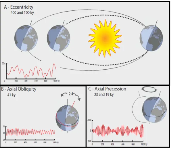
Fig. 1. Schematic representation of the Earth’s orbital cycles (adapted from Zachos et
al., 2001). (A) Changes in the eccentricity of the Earth’s orbit, with periods of 400 and 100 ka. (B) Variations in the obliquity, or tilt of the Earth’s axis, with amplitude of 2.4o every 41ka. (C) Precession, that corresponds to changes in the direction of the Earth’s axis relative to the fixed stars, with periods of 23 and 19 ka.
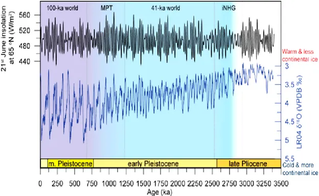
Fig. 2. Orbitally induced 100 ka and 41 ka climatic oscillations. In the top of the figure,
Summer solstice insolation at 65 ºN (Laskar et al., 2004). The Benthic foraminiferal δ18O stack of the last 3.5 Ma (Lisiecki and Raymo, 2005) shows a general cooling trend and an increase of global ice volume over the past 3 Ma (from Naafs, 2011). iNHG refers to the intensification of the NH glaciations and MPT refers to the middle Pleistocene transition.
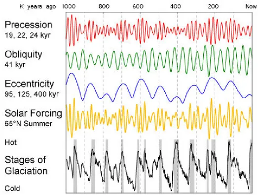
Fig. 3. Each orbital parameter is shown over the last 1000 ka along with the insolation
and stages of glaciation. The Milankovitch cycles have influenced climate change in 100 ka periods and determined the frequency of Quaternary glaciations (Berger, 1978).
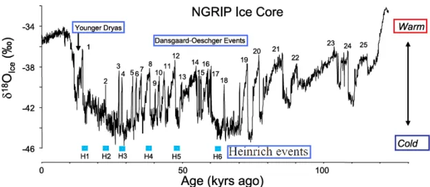
Fig. 4. North Greenland Ice Core Project (NGRIP) ice core δ18O record for the last 123
ka. The abrupt cooling reflecting the Younger Dryas corresponds to the Greenland stadial 1. The rapid warmings that characterize the D/O interstadial events are numbered from 1 to 25. Heinrich events are labeled from H1 to H6. Some stadials coincide with Heinrich events (from NGRIP members, 2004).
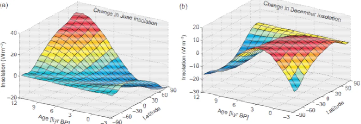
Fig. 5. Variations in orbital forcing during the Holocene (from 12 ka BP to 3 ka in the
future) in June (a) and December (b) as a function of latitude (from Beer and Geel, 2008). In June there is a strong decreasing trend in the north (a). In December, the insolation on the southern Hemisphere first increases and then reaches its maximum between 2 and 4 cal. ka BP before decreasing again (b).
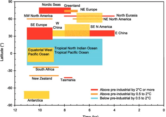
Fig. 6. Timing and intensity of maximum temperature deviation from pre-industrial
levels, as a function of latitude and time (from IPCC, 2007). It is suggested a possible south to north pattern, with southern latitudes showing HTM a few millennia earlier than the NH regions (IPCC, 2007).
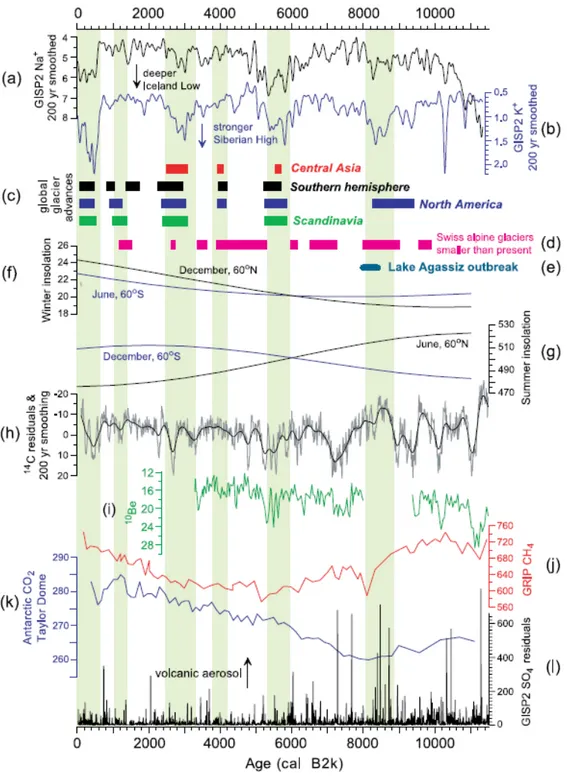
Fig. 7. Globally distributed glacier fluctuation records and climate forcing time series
aerosols, and greenhouse gases). Green bands represent timing of rapid climate change (RCC) identified by Mayewski et al. (2004) by tuned to GISP2 (Greenland Ice Sheet Project 2) record. For more details see Mayewski et al. (2004).
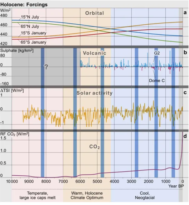
Fig. 8. Main external forcings driving Holocene climate changes (from Wanner et al.,
2011). Holocene long-term trend: (a) Solar insolation due to orbital changes for two specific latitudes in the Northern and Southern Hemispheres during the corresponding summer and d) Forcing due to rising CO2 concentrations. Holocene millennial scale
climate changes: (b) Volcanic forcing during the past 6 ka depicted by the sulphate concentrations of two ice cores from Greenland (blue vertical bars) and Antarctica (red vertical bars); (c) Solar activity fluctuations reconstructed based on 10Be measurements
in polar ice. The six vertical blue bars indicate the timing, but not the length of the six cold periods during the last 10 ka in the NH.
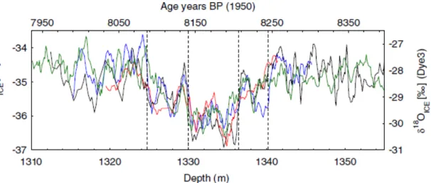
Fig. 9. Oxygen isotope ratios from GRIP (Greenland Ice Core Project) (red), GISP2 (black), NGRIP (blue), and Dye 3 (green) all plotted on the GRIP depth scale and the GICC05 age scale (from Thomas et al., 2007).
Fig.10. Configuration of the Northeast Canada and adjacent seas (from Barber et al.,
1999). Former ice-sheet margins are shown for 8.9 ka and 8.2 ka prior to present time (vertical hatched line and thick grey line respectively), before and after disintegration of ice in Central Hudson Bay, respectively. Simultaneously, northward drainage is shown through the Hudson Bay and Hudson Strait (dark grey arrows). Horizontal hatching shows Lake Agassiz and Ojibway. Labrador Sea current patterns and the area of Labrador Sea Intermediate Water (LSW) formation is indicated by arrows with dashed lines show. Numbers in boxes are regional mean DR values (years). Sites discussed in Barber et al. (1999) are numbered from 1 to 4.
Fig.11. Extra-tropical NH (90–30°N) temperature anomaly reconstruction of the last
2000 years (from Ljungqvist, 2010).
Fig. 12. Map showing the location of the studied core. The bathymetry is derived from
the Digital Bathymetry as produced in the EMODNet Hydrography (http://www.emodnet-hydrography.eu). The elevation data is derived from SRTM (Shuttle Radar Topography Mission) 90m Digital Elevation Database v4.1 (Farr et al., 2007). The drainage system is derived from the Europe and North Asia (EURNASIA) Vmap Level Zero (VMAP0 - Digital Chart of the World) (http://webgis.wr.usgs.gov/globalgis/metadata_qr/metadata/perennial_rivers.htm).
Fig. 13. Photos of KS05 10 core.
Fig. 14. Schematic representation of the Meridional overturning circulation (from
Rahmstorf, 2007). Global circulation system in the world ocean that shows the northward transport of warm and salty surface waters in the NA and the return flow to the south of cold and dense NADW in the abyssal ocean.
Fig. 15. Composition of ENACW circulation in the Bay of Biscay and the nearest part
Fig. 16. Based on the method described by Barnston and Livezey (1987) it is possible to
compute the spatial patterns associated to the teleconnection indices NAO, EA, and SCAND for DJF and for the period 1960-2000 (from Trigo et al., 2008).
Fig. 17. The two phases of the North Atlantic Oscillation. a) Positive phase, stronger
than average westerlies and to mild and wet winters over N-Europe and dry conditions in the Mediterranean; b) Negative phase, leading to the opposite conditions such as weaker than average westerlies, cold, dry winters in N-Europe and rainy winters in S-Europe (from http://www.ldeo.columbia.edu/NAO by Martin Visbeck).
Fig. 18. Spatial correlation between the patterns EA/WRUS and SCAND patterns and
winter (NDJF) Mediterranean station precipitation for the period 1950-1999. Correlations |r|≥0.14 indicate significance at the 95% level, |r|≥0.18 at the 99% level and |r|≥0.23 at the 99.9% level (n = 4x50 = 200 months), respectively (adapted from Trigo et al., 2006).
Fig. 19. Iberian Peninsula Bioclimatic (a) and Biogeographic map (b) (from Worldwide
Bioclimatic Classification System, 1996-2009). The Iberian Peninsula show marked differences between the two bioclimatic zones. The north and the northwest of the Peninsula are characterized by a Temperate bioclimate, with colder temperatures and higher precipitation than that of the Mediterranean bioclimatic. The small patches of Temperate bioclimate enclosed in the Mediterranean type correspond to large Mountain ranges in the centre and north of Iberia.
Fig.20. Details of angiosperm pollen wall structure as defined by Faegri (1956)
(adapted from Heusser, 2005).
Fig. 21. Groups of pollen according to the number, type and position of apertures (from
Moore et al., 1991). Examples are shown in equatorial view (view of a pollen grain where the equatorial plane is directed towards the observer) and polar view (the polar axis is directed towards the observer).
Fig. 22. Wall structure and ornamentation of angiosperm pollen (from Heusser, 2005).
Chapter 2
Fig. 1. Location of the study area and site (KS05 10; 43°22’765N, 2°16’744W).
Sources: The bathymetry is derived from the Digital Bathymetry as produced in the EMODNet Hydrography (http://www.emodnet-hydrography.eu). The elevation data is derived from SRTM (Shuttle Radar Topography Mission) 90m Digital Elevation Database v4.1 (Farr et al., 2007). The drainage system is derived from the Europe and North Asia (EURNASIA) Vmap Level Zero (VMAP0 - Digital Chart of the World) (http://webgis.wr.usgs.gov/globalgis/metadata_qr/metadata/perennial_rivers.htm).
Fig. 2. Sources and solid fluxes to the Spanish Basque country shelf (adapted from
Fig. 3. Depth-age model of KS05 10 record.
Fig. 4. Synthetic percentages pollen diagram against calibrated ages (cal. yr BP) of
KS05 10 record, with a curve at × 10 beyond the principal curve. Dots indicate percentages of less 0.5%.
Fig. 5. KS05 10 pollen record with Corylus, Cyperaceae, ubiquist plant group,
temperate and humid trees and Carpinus pollen percentage curves from 6500 to 9000 cal. yr BP.
Fig. 6. Correlation between vegetation changes, June insolation curve at 39ºN and
precessional signal (after Berger, 1978), δ18O-isotope composition of the NorthGRIP
ice-core (Johnsen et al., 2001; NGRIP Members, 2004; Rasmussen et al., 2006) and Sea surface temperature (SST) of Tagus mud patch (Rodrigues et al., 2009) during the last ca. 9000 cal. yr BP. Herbaceous plants association include: Ericaceae, Calluna, Ulex-type, Anthemis-Ulex-type, Aster-Ulex-type, Centaurea cyanus-Ulex-type, Centaurea nigra-Ulex-type, Taraxacum, Apiaceae, Brassicaceae, Caryophyllaceae, Liliaceae, Asphodelus, Mercurialis-type, Plantago, Plumbaginaceae, Poaceae, Ranunculaceae, Rumex, Saxifragaceae, Scabiosa, Boraginaceae, Campanulaceae, Cerealia-type, Cyperaceae, Euphorbia, Fabaceae, Filipendula, Galium-type, Gentianaceae, Geranium, Pedicularis, Polygonum aviculare-type, Rosaceae, Thalictrum, Helianthemum, Urtica, Valerianaceae, Armeria-type, Eleagnaceae, Polygonaceae and Potentilla-type.
Fig. 7. Correlation between KS05 10 vegetation changes, δ18O-isotope composition of
the NorthGRIP ice-core (Johnsen et al., 2001; NGRIP Members, 2004; Rasmussen et al., 2006), negative SST anomalies in the Tagus mud patch (Rodrigues et al., 2009), mean grain size (paleocurrent flow speed proxy, higher mean indicates stronger flow of the depositing current and vice versa; Ellison et al., 2006), the catastrophic final drainage episodes from the proglacial Laurentide lakes into the Hudson Bay at ca. 8470 cal. yr BP (error range of 8160–8740 cal. yr BP; Barber et al., 1999) and episodes of higher lake level in west-central Europe (Magny, 2007), during the 8.2 ka cooling event.
Fig. 8. Comparison of hydrological signals related to the 8.2 ka cold event in Europe
(from Magny et al., 2003). Shaded area represents the mid-European zone with wetter conditions. Lake-level maxima is marked with (+) and minima with (-) during the 8.2 ka event. The extension of sea-ice cover during the 8.2 cal. yr BP (Renssen et al., 2001). Dashed lines correspond to possible northern and southern limits of the mid-European wetter zone during the Holocene cooling phases weaker than the 8.2 ka event. X marks the location of KS05 10 sequence. For reference sites included in the Fig. during the 8.2 ka event see Magny et al. (2003).
Fig. 9. The mean 500 hPa geopotential height (gpm) anomalies for all winter a)
blocking, and, b) non-blocking (strong zonal flow) episodes, with a minimum duration of 10 days (from Trigo et al., 2004b). The shading shows the corresponding 850 hPa temperature field (ºC); c) Differences between the mean 500 hPa geopotential height (gpm) composites and the corresponding 850 hPa (ºC) temperature composites (represented only if significant at the 1% level).
Fig. 10. Number of cyclones per winter, detected per 5º x 5º area normalised for 50ºN,
for a) blocking, b) non-blocking, and c) their difference (from Trigo et al., 2004b).
Fig. 11. Anomalies of the precipitation rate (mm/day) for winter composites of a)
blocking episodes, b) non-blocking episodes, and c) their difference (represented only if significant at the 5% level). The arrows show the respective anomaly of the 2.5 m wind field (ms–1) (adapted from Trigo et al., 2004b).
Fig. 12. Wavelet analysis of the hazel percentages for the last ca.9000 yr. Wavelet
power spectra illustrate the change in concentration of spectral power with time in Corylus values. Black line defines power spectrum significant at 90% red noise spectrum. Dashed lines define the cone of influence where the spectrum has no significance at all. Analysis undertaken using interactive software available at http://paos.colorado.edu/research/wavelets/.
LIST OF TABLES
Chapter 1
Table 1. The Holocene three main periods (adapted from Nesje and Dahl, 1993;
Marchal et al., 2002; Wanner et al., 2008; 2011).
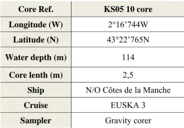
Table 2. Main features of the cored site.
Chapter 2
Table 1. Results of AMS dating of core KS05 10. Level in italic corresponds to the age
not considered for the age model.
Table 2. Historical botanic event.
Table 3. Description of pollen zones from the well-dated KS05 10 sedimentary
Chapter I
1. MAIN OBJECTIVES AND MOTIVATION
Climate is changing significantly since the last few decades, affecting people and the environment worldwide. In particular, increasing air and ocean temperatures, widespread melting of snow and ice, and rising sea levels result in a shift in the Earth’s climate system equilibrium. Natural events and human activities are believed to be contributing to this climatic trend. Differentiating natural from anthropogenic forcing of climate change is one of the most important challenges of future climate prediction. There is therefore an urgent need to improve our documentation and understanding of natural variability for periods stretching back beyond the instrumental record. From this perspective, it is of extreme importance to know more about natural climate variations that occurred during the current interglacial, the Holocene, because its boundary conditions are similar to those experienced now and in the near future.
Growing evidence suggests that variations in Holocene climate were larger than previously believed. In the last few years, numerous studies have been performed on several naturally occurring archives such as lake and marine sediments, tree rings, speleothems and ice cores to understand the nature, timing and causes of Holocene natural climate oscillations. Such studies have shown that superimposed on the orbitally-induced long-term cooling sub-orbital millennial-scale climate variability has affected this interglacial.
The most extreme short-lived cold episode noticed in the Greenland Ice cores, the “8.2-kyr-BP event”, lasted 100-200 years and has been detected elsewhere in the North Atlantic and in Europe. Several hypotheses have been invoked to explain this cooling such as: a) significant alterations of solar activity or b) changes in general circulation pattern of the North Atlantic region. The first hypothesis suggest a reduction of the solar activity as the result of increasing sunspots while the second hypothesis suggest that this cooling was triggered by the final catastrophic drainage of the Lakes Agassiz and Ojibway which contributed to the introduction of large amounts of freshwater into the North Atlantic Ocean, disturbed the thermohaline circulation and cooled both Europe and North America. In recent years, few studies have shown that this event was longer and more complex than previously believed. Yet, the spatial distribution, timing, amplitude and their impact in the ecosystems remains one of the outstanding mysteries of climate variability. Also, the 8.2 ka event is seen as the best analogue for the “worst case” scenario for the future. Thus, the global warming is accelerating the melting of the Greenland ice sheet which is contributing to a drastic increase of the global sea level,
threatening low-lying areas around the globe with beach erosion, coastal flooding, and contamination of freshwater supplies. As this ice melts, voluminous amounts of cold, fresh water dump into the world's oceans disrupting the general trend of the global oceanic circulation leading to an extreme cooling over Europe and North America. Understanding the changes in the frequencies and intensities of extreme climate events and weather, as well as in sea level rise, is therefore a necessity for reducing adverse impacts on natural and human systems.
In contrast, the signature of millennial-scale climate changes during the mid- and late Holocene (after the “8.2 ka event”) is not easily detected in paleoclimatic records. However, this variability was strong enough to affect human societies, particularly during the last millennium, as historically documented for the Little Ice Age (LIA) and the Medieval Warm Period (MWP). The global impact, amplitude, periodicities and causes triggering these short-lived climatic oscillations have been widely discussed in thelast decade.
There is therefore an urgent need to understand the nature, timing and causes of climate oscillations and to determine how widespread, systematic and abrupt they may have been.
Most of the available Holocene climatic reconstructions are however, not based on good correlation between terrestrial, marine and ice records making it difficult to get an accurate understanding of the interactions of the atmosphere-ocean-land systems and their impact on global climate variability. For this reason, the mechanisms that control Holocene climate variations in the North Atlantic and adjacent landmasses are far from being resolved. We propose, therefore, to establish for the first time, high-resolution sea-land correlation on a shelf core from southwestern France (highlighted by the IPCC models as one of the most sensitive region to the ongoing global climatic changes) covering the Holocene.
This master thesis aims to improve the understanding of the nature, timing and causes of Holocene natural climate oscillations and to determine how abrupt they may have been. Furthermore, this thesis aims to document how changes in the behaviour of coupled atmosphere-ocean-land systems have affected climate in the North Atlantic region during the Holocene. In particular we pretend:
a) to document the response of vegetation to Holocene climate changes in terms of long and millennial scale and in particular:
- to determine the impact of long term cooling in the vegetation cover of both northern Iberian Peninsula and southwestern France;
- to determine the impact of the 8.2 ka event in both northern Iberian Peninsula and southwestern French margin;
- to determine the trigger mechanisms involved in the climatic signal left by the 8.2 ka in southwestern French margin/northern Spain;
- to determine the impact of less extreme events in the northern Iberian Peninsula and southwestern France and to determine, if possible, the cyclicities within the sub-orbital climatic oscillations in terrestrial environments and to determine the trigger mechanisms involved in those changes;
b) to compare the obtained marine pollen data with other marine paleoclimatic and ice records to further understand the nature, amplitude and timing of millennial-scale climate variability in northern Iberian Peninsula and southwestern France;
c) to understand if the sub-orbital millennial-scale climate oscillations had contributed to an amplification or reduction of the long-term climatic signal;
To achieve theses aims, I have organised the work with the following sequence of steps: 1. Obtain high-resolution data and high-quality chronology
High time-resolution analyses enabled by both high sedimentation rate marine cores and well chronologically constrained records (using several AMS 14C dating) are a prerequisite to investigate the rapid climatic variability of the Holocene.
2. Document the Holocene southern European vegetation changes
Pollen, representing an integrated image of the regional vegetation of the borderlands, will be analysed.
3. Integrate terrestrial and marine data results
An accurate correlation of marine and terrestrial settings is of prime importance for time equivalent documentation of environmental changes and to evaluate the synchronicity of occurring climatic shifts and events in both environments.
4. Implement cyclicity analysis of the marine and terrestrial records
This task will allow us to determine the main trigger mechanisms involved in the Holocene millennial scale climatic variability.
5. Evaluate the natural and anthropogenic contributions to the Holocene climatic changes.
2. CLIMATE VARIABILITY DURING THE LATE QUATERNARY
During the late Quaternary (roughly the last million years) global climate has changed dramatically due to a number of linked physical, chemical and biological processes occurring in the atmosphere, land and ocean.
Changes in Earth’s orbit (Milankovitch cycles) as well as oscillations in solar activity determine the temporal and spatial distribution of insolation, being considered the ultimate forcing of the long-term climate oscillations of the Quaternary. Additionally, Earth’s internal mechanisms that result from the interaction between atmosphere-ocean-lithosphere-cryosphere-land systems have a huge contribute to the climatic changes. The variability of these global phenomena may trigger, amplify, sustain or globalize rapid climatic fluctuations (Peixoto and Oort, 1992).
2.1 Long term climate variability (Glacial-Interglacial cycles)
Over the last million years, the earth’s climate system has experienced several long term climatic shifts between glacial and interglacial conditions which were mainly controlled by solar irradiance variations linked to changes in the Earth’s orbit around the sun (Milankovitch, 1920; Berger, 1978; Imbrie et al., 1992; Berger and Loutre, 2004; Ruddiman, 2006). Changes in the amount of incoming solar radiation, as well as their temporal and spatial distribution are determined by three types of orbital parameters (Milankovitch, 1920) (Fig. 1):
(1) Eccentricity, reflects the shape of Earth's orbit around the Sun, ranging from a quasi-circular (low eccentricity of 0.0006) to a slightly elliptical shape (high eccentricity of 0.0535) and with two periodicities of about 100 and 400 thousands of years (kilo years, hereafter referred to as ka) (Berger and Loutre, 1992; Berger and Loutre, 2004). Differences in solar radiation received on earth of about 30% may occur between perihelion (in early January, when the Earth is closest to the sun) and aphelion (in early July, when the Earth is further from the sun) during eccentricity maxima (Goodess et al., 1992). In contrast, during episodes of low eccentricity (0.016) as the present-day, the difference in insolation between perihelion and aphelion is around 6.4 % over the year (Berger, 2001).
(2) Obliquity of Earth’s axis in relation to the orbital plan, tilting from 22° and 25° over a period of about 41 ka (Berger and Loutre, 2004), determine the differences in seasonal contrast on earth (Buchdahl, 1999). Increased obliquity implicates a higher seasonal contrast in both hemispheres at high latitudes, since summers receive more solar radiation and winters less (i.e. warmer summers/colder winters). Inversely, decreased obliquity origin temperate summers and milder winters, which is the most likely mechanism promoting the onset of glacial conditions favoring the ice cap growth in the high latitudes. Fluctuations in obliquity have less influence at low latitudes, as the strength of the effect decline towards the equator (Buchdahl, 1999).
(3) precession (change in the orientation of the Earth's rotational axis) is modulated by eccentricity, which splits the precession into two periods of about 23 ka and 19 ka, leading to an average period of 21 ka (Berger, 2001; Berger and Loutre, 2004). This cycle has two components: an axial precession, caused by the gravitational forces exerted on Earth of all other planetary body's in our solar system, and an elliptical precession, in which the elliptical orbit of the Earth itself rotates about one focus (Buchdahl, 1999). Changes in axial precession modify the times of perihelion and aphelion, and consequently increase the seasonal contrast in one hemisphere and decrease in the other hemisphere. The hemisphere at perihelion experiences an increase in summer solar radiation and a cooler winter, while the opposite hemisphere will have a warmer winter and a cooler summer. Presently, the Earth is at perihelion in the northern hemisphere (hereafter referred to as NH) winter, which makes the winters and summers less severe in this region (Ruddiman, 2001).
Orbital forcing is the only forcing that is fully understood, and can be calculated not only for the past but also for the future several million years (Berger and Loutre, 2004). Isolated or combined together, the orbital parameters shape the distribution of solar radiation in Earth’s surface. Whereas eccentricity is the only Milankovitch cycle that modify the annual-mean global solar insolation at aphelion and perihelion; the seasonal and latitudinal variation of the incoming radiation is balanced by precession and obliquity respectively.
Fig. 1. Schematic representation of the Earth’s orbital cycles (adapted from Zachos et al., 2001). (A) Changes in the eccentricity of the Earth’s orbit, with periods of 400 and 100 ka. (B) Variations in the obliquity, or tilt of the Earth’s axis, with amplitude of 2.4o every 41ka. (C)
Precession, that corresponds to changes in the direction of the Earth’s axis relative to the fixed stars, with periods of 23 and 19 ka.
The timing, duration and amplitude of major glacial-interglacial cycles have been modulated by changes in the prevailing astronomical parameters. Thus, Early Pleistocene low-amplitude 41 ka obliquity-forced climate cycles were gradually replaced by later Pleistocene 100 ka eccentricity-forced climate cycles (Head and Gibbard, 2005) (Fig. 2). The transitional period occurring between the 41 ka and 100 ka cyclicities is known as the Mid Pleistocene Transition (MPT) (1.25-0.7 Ma) (Clark et al., 2006).
Fig. 2. Orbitally induced 100 ka and 41 ka climatic oscillations. In the top of the figure, Summer solstice insolation at 65 ºN (Laskar et al., 2004). The Benthic foraminiferal δ18O stack
of the last 3.5 Ma (Lisiecki and Raymo, 2005) shows a general cooling trend and an increase of global ice volume over the past 3 Ma (from Naafs, 2011). iNHG refers to the intensification of the NH glaciations and MPT refers to the middle Pleistocene transition.
This transition favored the gradual intensification (ice volume increase) and longer duration of glacial states (Imbrie et al., 1993) (Fig. 3). Interglacials before the Mid-Brunhes Event (MBE) at ~425 ka were less intense than post-MBE interglacials, meaning that temperatures were probably colder and sea level and CO2 concentrations
in the atmosphere were lower (Lisiecki and Raymo, 2005) (Fig.3). Thus, the last 1 Ma is characterized by long cold periods with massive continental ice-sheets and polar ice caps followed by short warmer stages with ice-free poles and sea level rising (Zachos et al., 2001).
Fig. 3. Each orbital parameter is shown over the last 1000 ka along with the insolation and stages of glaciation. The Milankovitch cycles have influenced climate change in 100 ka periods and determined the frequency of Quaternary glaciations (Berger, 1978).
2.2 Millennial-scale climate variability
Superimposed on the long term variability, the last glacial cycle is characterized by large, abrupt and widespread millennial-scale climatic changes, known as Dansgaard-Oeschger (D-O) events (Dansgaard et al., 1993) (Fig. 4). The D-O events are characterized rapid warming (Greenland interstadials - GIS) and gradual cooling episodes (Greenland stadials - GS), occurring every 1500 years (Dansgaard et al., 1993). During the last climate cycle, twenty five D/O events were detected in Greenland with atmospheric temperatures presenting a warming of 8ºC to 16ºC within several decades (e.g. Severinghaus and Brook, 1999; NGRIP members, 2004).
Some of those D-O stadials were extremely cold, occurring every 5-10 ka (Elliot et al., 1998), and are known as Heinrich events (Bond and Lotti, 1995). Heinrich events were first documented in several North Atlantic deep-sea cores between 45 and 50° N (Ruddiman belt) (Ruddiman, 1977; Heinrich, 1988; Bond and Lotti, 1995) and identified by the anomalous presence of ice-rafted detritus (IRD) that were transported
to the ocean by drifting icebergs from the Laurentide and northern European ice sheets as well as by synchronous peaks of polar foraminifera, N. pachyderma (s) (e.g. Bond and Lotti, 1995; Hemming, 2004), sea surface temperature decreases (Bond and Lotti, 1995; Cortijo et al., 1997) and magnetic susceptibility peaks (Grousset et al., 1993). These coarse fraction intervals, representing the well known IRD layers, were also detected beyond the Ruddiman belt i.e. north of 50°N (e.g. Elliot et al., 1998; Fronval et al., 1995; Rasmussen et al., 1996; Van Kreveld et al., 2000; Voelker et al., 1998) as well as below 40°N (e.g. Baas et al., 1997; Bard et al., 2000; Chapman et al., 2000; de Abreu et al., 2003; Lebreiro et al., 1996; Zahn et al., 1997; Naughton et al., 2009). The thickness of the IRD layers and the magnetic signal is, however, smaller in the mid-latitude sites than in the northern ones (Thouveny et al., 2000). Also, the duration of the impact of these extreme events on the sea surface temperatures (SST) in this region is longer than that of the IRD layers (e.g. Bard et al., 2000; Chapman et al., 2000; Sánchez Goñi et al., 2000; Naughton et al., 2009). Moreover, the vegetation patterns within these extreme cold events are also complex in southwestern Europe (Naughton et al., 2009).
Internal mechanisms have been invoked to explain Heinrich climatic anomalies. Thus, the introduction of anomalous freshwater pulses into the North Atlantic have affected the general pattern of the global thermohaline circulation (THC), by forcing the THC to slowdown (almost shutdown) (e.g. Ganopolski and Rahmstorf, 2001; Knutti et al., 2004), triggering a substantial SST drop in the North Atlantic region and extreme cooling in Europe (e.g. Paillard and Labeyrie, 1994; Seidov and Maslin, 1999). The slowdown/shutdown of the THC also precludes the moisture transfer to Europe. Following this, rapid oceanic and atmospheric reorganizations favoured the transfer of cold conditions everywhere on earth suggesting that although Heinrich events were mainly North Atlantic (hereafter referred to as NA) phenomena they had a global impact (Leuschner and Siroko, 2000; Voelker et al., 2002). Several other hypotheses have been invoked to explain the response of the ocean-land-ice to Heinrich events (e.g. Flückiger et al., 2006; Sánchez Goñi et al., 2002; Naughton et al., 2009). However, despite the recent paleodata acquisition and modelling efforts, understanding of the mechanisms that give rise to theses instabilities is far from being completely understood (Hemming, 2004).
Fig. 4. North Greenland Ice Core Project (NGRIP) ice core δ18O record for the last 123 ka. The abrupt cooling reflecting the Younger Dryas corresponds to the Greenland stadial 1. The rapid warmings that characterize the D/O interstadial events are numbered from 1 to 25. Heinrich events are labeled from H1 to H6. Some stadials coincide with Heinrich events (from NGRIP members, 2004).
The millennial-scale fluctuations were largest when glacial ice sheets existed in the NH, and they have been less significant during interglacial climates as the present one (Ruddiman, 2001). Nevertheless, the mechanisms and causes that drive these abrupt changes are not totally understood and remain one of the greatest challenges in climate research.
2.3 The Holocene
For a long time the Holocene (present-day interglacial; past 11,7 ka) was considered a period of stable warm climatic conditions (e.g. Dansgaard et al., 1993; McManus et al., 1999). However, in the last few years a wide array of different high-resolution paleoclimatic records such as lake and marine sediments, peat bogs, tree rings, speleothems and ice cores together with climate simulations have shown that a long term and millennial scale climate variability has affected this interglacial (e.g. Kutzbach and Gallimore, 1988; Bond et al., 1997; 2001; Crucifix et al., 2002; Weber and Oerlemans, 2003; Mayewski et al., 2004; Renssen et al., 2005; Wanner et al., 2008; 2011).
2.3.1 Holocene long term climatic changes
The decrease in the northern high-latitudes summer insolation along the Holocene induced a long-term cooling trend in the NH confirming that orbitally induced changes in NH insolation is the major driver of long-term climate variations during the Holocene (Kutzbach and Gallimore 1988; Braconnot et al,. 2000; Duplessy et al., 2001; Johnsen et al., 2001; Crucifix et al,. 2002; Marchal et al., 2002; Andersen et al., 2004; Kim et al., 2004; Moros et al., 2004; Solignac et al., 2004; Weber et al., 2004; Renssen et al., 2005; Keigwin et al., 2005).
During the Holocene, the insolation changes are dominated by the effect of precession and obliquity astronomical parameters. Fig. 5 clearly shows the seasonal hemispheric insolation changes as a function of latitude, with the summer insolation curves of both hemispheres exhibiting an opposite behavior. In the NH the summer insolation slightly increase by the beginning of the Holocene with a peak around 11-10 ka BP (BP means "before present" and 0 BP represents 1950 AD) and afterward decreases towards modern values. The NH winter insolation shows a change in the opposite direction with a steady raise since the beginning of the Holocene.
Fig. 5. Variations in orbital forcing during the Holocene (from 12 ka BP to 3 ka in the future) in June (a) and December (b) as a function of latitude (from Beer and Geel, 2008). In June there is a strong decreasing trend in the north (a). In December, the insolation on the southern Hemisphere first increases and then reaches its maximum between 2 and 4 cal. ka BP before decreasing again (b).
The gradual increase of precession consequently induces a reduction of the NH seasonality during the Holocene. This is in agreement with climatic models of Holocene climate evolution that reveal an early optimum (9–8 ka BP) in the high northern latitudes followed by a gradual decrease in summer temperatures (1-3°C), a reduction in summer precipitation and the expansion of sea-ice cover (Renssen et al., 2005).
Nevertheless, the greenhouse gas forcing partly counteracts (+ 0.5° C) the decrease in summer insolation in the areas north of 60ºN over 9 ka (Crucifix et al., 2002; Renssen et al., 2005).
The orbital induced NA long term cooling of the Holocene is also accompanied by a southern shift of the Intertropical Convergence Zone (ITCZ) and a weakening of the NH summer monsoon systems (Mayewski et al., 2004; Braconnot et al., 2007; Wanner et al., 2008; 2011).
Besides the long term cooling, the Holocene is divided in three main periods (Table 1): The early Holocene deglaciation (~ 11.7 - 7 ka BP), Holocene Thermal Optimum (~ 7 - 4.2 ka BP) and Neoglacial (~ 4.2 ka BP - pre-industrial time) (e.g. Nesje and Dahl, 1993; Marchal et al., 2002; Wanner et al., 2008; 2011).
Period
Main features
Early Holocene deglaciation
Climatic amelioration when compared with the previous glacial period. This includes the North European “Preboreal” and “Boreal” chronozones.
- High NH summer insolation. The insolation maximum occurred at around 11 ka BP due to a coincidence of the appropriate phases of both precession and obliquity cycles.
- Deglaciation of the North America and Eurasia ice sheets triggering a slight cooling effect at least at a regional scale.
- High monsoon activity in Africa and Asia. - Strong sea level rise.
Holocene Thermal Optimum
Relatively warm period called “Holocene Climate Optimum” and “Hypsi- or Altithermal”, which also includes the North European “Altantic” chronozone.
- Decreasing NH summer insolation, southward displacement of the ITCZ.
- Summer temperatures in the NH mid- and high-latitude regions are higher than during the pre-industrial period (prior to year 1900 AD). - North American ice sheet is no longer large enough to influence climate at a hemispheric scale.
- Most of the global monsoon systems still active, but weaker. - Major sea level changes ceased after ~6 ka BP.
Neoglacial
Rather cold phase that coincides with the North European “Subboreal” and “Subatlantic” chronozones.
- Low values of NH summer insolation leading to a decrease in summer temperatures.
- Occurrence of several cold relapses with remarkable glacier advances in different areas of the globe.
- Sea ice increases in the high latitudes.
- The Neoglacial period was interrupted by the global warming driven by anthropogenic forcing (increased anthropogenic greenhouse effect), therefore it lasted until the beginning of industrialization.
Table 1. The Holocene three main periods (adapted from Nesje and Dahl, 1993; Marchal et al., 2002; Wanner et al., 2008; 2011).
Note: The Holocene has been subdivided into five time intervals, or chronozones, based on Northern European climatic stratigraphies (Preboreal, Boreal, Atlantic, Subboreal and Subatlantic). The Hypsi- or Altithermal refers to warm conditions in northern mid- to high latitudes. Nevertheless these terms are related to regional climatic fluctuations and have not been consistently applied (Wanner et al., 2008).
Although summer insolation in the NH decreased after ~11-10 ka BP, the timing and magnitude of the Holocene Thermal Maximum (hereafter referred to as HTM) was not synchronous across the hemisphere (Fig. 6), suggesting the involvement of extra feedbacks and forcings (e.g. Kaufman et al., 2004; Renssen et al., 2005; IPCC, 2007; Renssen et al., 2009). The HTM was detected at the beginning of the Holocene (~11-8 ka BP) in several paleoclimatic studies of the NA and adjacent Arctic (Duplessy et al., 2001; Andrews and Giraudeau, 2002; Marchal et al., 2002; Kaufman et al., 2004; Kim et al., 2004; Knudsen et al., 2004; Vernal et al., 2005; Kaplan and Wolfe, 2006). Also, the Iberian margin records, located at the mid-latitudes of the NA, clearly show an early Holocene thermal maximum (Bard et al., 2000; Pailler and Bard, 2002; Rodrigues et al., 2010) synchronous with the maximum expansion of temperate trees in the adjacent landmasses (Turon et al., 2003; Naughton et al., 2007a). However, other proxy data from northern high latitudes indicate that the HTM occurred considerably later, after ~8 ka (Dahl-Jensen et al., 1998; Korhola et al., 2000; Johnsen et al., 2001; Levac et al., 2001; Kaufman et al., 2004; Solignac et al., 2004; Keigwin et al., 2005; Kaplan and Wolfe, 2006). In Europe and north-western North America the Holocene maximum warmth was observed between 8 and 4 ka BP (Davis et al., 2003; Kaufman et al., 2004).
Fig. 6. Timing and intensity of maximum temperature deviation from pre-industrial levels, as a function of latitude and time (from IPCC, 2007). It is suggested a possible south to north pattern, with southern latitudes showing HTM a few millennia earlier than the NH regions (IPCC, 2007).
2.3.2 Holocene millennial to sub-millennial scale climate variability
Superimposed on the orbital induced long-term cooling trend a series of relatively cold events punctuated the Holocene. Denton and Karlén (1973) have suggested that advances of the Northern Europe and America mountains glaciers had responded to millennial scale climate coolings; O’Brien et al., (1995) have showed that Holocene atmospheric circulation above the ice cap of Greenland ice sheets was disturbed by a series of millennial scale shifts. Encouraged by these evidences Bond et al., (1997) have launched a deep sea sedimentary research in the NA revealing the presence of IRD (Ice rafted detritus) and a decrease in the sea surface temperatures during the coldest phases of this millennial scale variability. Following these pioneer works, these short-lived climate oscillations have been detected in a variety of paleoclimatic archives such as ice, marine and terrestrial records (Fig. 7) (e.g. Mayewski et al. 2004; Wanner et al., 2008; 2011).The timing of millennial-scale climate oscillations detected in the NA region during the Holocene is of about 2800-2000 and 1500 yr (e.g. Denton and Karlén, 1973; O’Brien et al., 1995, Bond et al., 1997; 2001, Mayewski et al., 2004).
Fig. 7. Globally distributed glacier fluctuation records and climate forcing time series (cosmogenic isotopes reflecting solar variability, orbital insolation changes, volcanic aerosols, and greenhouse gases). Green bands represent timing of rapid climate change (RCC) identified by Mayewski et al. (2004) by tuned to GISP2 (Greenland Ice Sheet Project 2) record. For more details see Mayewski et al. (2004).
A number of processes such as solar activity, volcanic eruptions and internal oscillations of the climate system driven by land-ocean-atmosphere interactions have been put forward to explain the millennial-scale variability (e.g. Mayewski et al., 2004; Wanner et al., 2011) and references therein for a comprehensive overview) (Fig. 8).
In the NH the most important internal variations of the climate system include the Arctic Oscillation/North Atlantic Oscillation (e.g. Hurrell, 1995, hereafter referred to as AO/NAO), the Atlantic Multidecadal Oscillation, the Pacific Decadal Oscillation and the variations in the NA thermohaline circulation (hereafter referred to as THC). In terms of the major phenomena in the Atlantic, it is important to note that during the past 6 ka there is evidence for a continuous SST decrease in the NA and a negative trend (weakening) in the NAO index (Rimbu et al., 2003; Wanner et al., 2008). According to Rimbu et al. (2003) NAO may have played a role in generating millennial-scale SST trends, with the positive (negative) phase accompanied by relatively mild (cold) winters over northern Europe and a relatively cold (warm) climate in the eastern Mediterranean and the Middle East.
Fig. 8 shows the four most important external climate forcing factors during the Holocene and six cold relapses with no clear cyclicity (8200, 6300, 4700, 2700, 1550 and 550 years BP) recognized by Wanner et al. (2011) at multidecadal to multicentury scale in the NH. The complex spatiotemporal pattern of the cold relapses may be a consequence of different dynamical processes such as low solar activity, combined with a meltwater flux into the NA, a possible slowdown of the thermohaline circulation and, in some cases, series of large tropical volcanic eruptions (Wanner et al., 2011). Moreover, feedback mechanisms may have been important, in particular when regional or even local phenomena are studied. Thus, although the global impact, amplitude, periodicities and causes triggering these short-lived climatic oscillations have been widely discussed in the last decade (e.g. Risebrobakken et al., 2003; Mayewski et al., 2004; Andrews, 2006; Debret et al., 2007; Wanner and Bütikofer, 2008; Wanner et al., 2008; 2011) the spatial distribution of those millennial-scale climatic patterns and the origin of this pacing during the Holocene remains one of the outstanding mysteries of climate variability. There is therefore an urgent need to understand the nature, timing and causes of climate oscillations and to determine how widespread, systematic and abrupt they may have been.
Fig. 8. Main external forcings driving Holocene climate changes (from Wanner et al., 2011). Holocene long-term trend: (a) Solar insolation due to orbital changes for two specific latitudes in the Northern and Southern Hemispheres during the corresponding summer and d) Forcing due to rising CO2 concentrations. Holocene millennial scale climate changes: (b) Volcanic
forcing during the past 6 ka depicted by the sulphate concentrations of two ice cores from Greenland (blue vertical bars) and Antarctica (red vertical bars); (c) Solar activity fluctuations reconstructed based on 10Be measurements in polar ice. The six vertical blue bars indicate the
2.3.2.1 Particular cases of well known Holocene short-lived climatic events
The most extreme Holocene short-lived cold episode occurred at around 8200 yr BP and is known as the 8.2 ka cooling event. The 8.2 ka event is characterized by a evident cooling of about 3.3 +/-1.1ºC during ~160 yr in Greenland ice core records (Fig. 9), coinciding with a reduction in ice accumulation rate, increasing wind speeds and a decline in atmospheric methane concentrations. (O'Brien et al., 1995; Alley et al., 1997; Muscheler et al., 2004; Kobashi et al., 2007; Thomas et al., 2007). This event was also detected in many other terrestrial (e.g. Klitgaard-Kristensen et al., 1998; Von Grafenstein et al., 1998; Magny et al., 2003) and marine records (e.g. Bond et al., 1997; 2001; Keigwin and Boyle, 2000; Alley and Ágústsdóttir, 2005 and references therein; Naughton et al., 2007b) of the NA region, as well as in areas influenced by monsoons suggesting the widespread signature of the abrupt 8.2 ka event (Alley and Ágústsdóttir, 2005; Rohling and Pälike, 2005; Fleitmann et al., 2007).
Fig. 9. Oxygen isotope ratios from GRIP (Greenland Ice Core Project) (red), GISP2 (black), NGRIP (blue), and Dye 3 (green) all plotted on the GRIP depth scale and the GICC05 age scale (from Thomas et al., 2007).
The causes triggering the 8.2 ka cold event have been largely debated in the last 15 years. Several authors suggest that “8.2 event” was triggered by the rapid collapse of the Hudson Bay dome of the Laurentide Ice sheet which result in a final catastrophic drainage of the Laurentide Lakes (Lake Agassiz and Ojibway) at around 8470 yr BP (Fig. 10) (Barber et al., 1999; Clarke et al., 2004). This phenomenon contributed to the introduction of large amounts of freshwater into the NA Ocean which disturbed the thermohaline circulation and the formation of the North Atlantic deep water (NADW)
(e.g. Alley et al., 1997; Clark et al., 2001; Clarke et al., 2004). The slowdown of the THC prevented the maintenance of the heat transport by the Gulf and NA currents to the high latitudes as showed by models simulations (Fawcett et al., 1997) generating a cooling and dryness of the NA and Europe (Broecker et al., 1985; 1990; Bond et al., 1997; Barber et al., 1999; Broecker., 2000; Cubasch et al., 2001; Renssen et al., 2001; Rind et al., 2001; Vellinga and Wood, 2002; Nesje et al., 2004; Wiersma and Renssen, 2006; Wiersma et al., 2006; Flesche Kleiven et al., 2008). This caused the weakening of the THC and associated northward oceanic heat flux, leading to a significant cooling in the NA (Fawcett et al., 1997; Rahmstorf, 2002). Additionally, these processes may have caused the spread of winter sea ice across the NA, thus causing the northern region to experience much colder winters which induced an increase in seasonality (Denton et al., 2005).
Fig.10. Configuration of the Northeast Canada and adjacent seas (from Barber et al., 1999). Former ice-sheet margins are shown for 8.9 ka and 8.2 ka prior to present time (vertical hatched line and thick grey line respectively), before and after disintegration of ice in Central Hudson Bay, respectively. Simultaneously, northward drainage is shown through the Hudson Bay and Hudson Strait (dark grey arrows). Horizontal hatching shows Lake Agassiz and Ojibway. Labrador Sea current patterns and the area of Labrador Sea Intermediate Water (LSW) formation is indicated by arrows with dashed lines show. Numbers in boxes are regional mean DR values (years). Sites discussed in Barber et al. (1999) are numbered from 1 to 4.