Clustering and forecasting of dissolved oxygen concentration on a river basin

(1)

UNCORRECT

ED

PROOF

O R I G I N A L P A P E R

1

2

Clustering and forecasting of dissolved oxygen concentration

3

on a river basin

4 _{Marco Costa}•A. Manuela Gonc¸alves

5

6 !Springer-Verlag 2010

7 Abstract The aim of this contribution is to combine

8 _{statistical methodologies to geographically classify} homo-9 _{geneous groups of water quality monitoring sites based on} 10 _{similarities in the temporal dynamics of the dissolved} 11 _{oxygen (DO) concentration, in order to obtain accurate} 12 _{forecasts of this quality variable. Our methodology intends} 13 _{to classify the water quality monitoring sites into spatial}

14 _{homogeneous groups, based on the DO concentration,}

15 _{which has been selected and considered relevant to} char-16 _{acterize the water quality. We apply clustering techniques} 17 _{based on Kullback Information, measures that are obtained} 18 _{in the state space modelling process. For each} homoge-19 _{neous group of water quality monitoring sites we model the} 20 _{DO concentration using linear and state space models,} 21 _{which incorporate tendency and seasonality components in} 22 _{different ways. Both approaches are compared by the mean} 23 _{squared error (MSE) of forecasts.}

24

25 _Keywords _{Hydrological basin}_{! Water quality !} 26 _Clustering_{! State space model ! Linear model !}

27 _{Kalman filter}

28 1 Introduction

29 As water is a precious asset as well as a potential inducer of

30 riches, water quality monitoring networks are important

31 tools in the management and assessment of surface water

32 quality and they could be improved by means of accurate

33 forecasts of the surface water variables. The European

34 Water Framework Directive (WFD) establishes a common

35 framework for sustainable and integrated management of

36 natural waters. This implies a high level of

multi-disci-37 plinary and a tight connection between water management

38 technical bodies and instruments of analysis for

decision-39 making (Vieira2003).

40 Surface waters in a river basin are usually submitted to

41 pressures and changes due to human activities. These

42 activities are one of the most important causes of the

43 degradation of water quality, which could pose risks for

44 public health. At a river basin scale there is a need to

45 establish a methodology for systematic data monitoring for

46 the characterization of surface water quality and for the

47 correct analysis of collected data, so that the present and

48 expected future pressures can be identified and understood.

49 Assessment of pressure-state impact interaction can be

50 facilitated using environmental indicator tools (Oliveira

51 et al. 2005).

52 In this work, we intend to contribute to the discussion

53 and understanding of an environmental issue of such

54 importance to the community, as is the case of the quality

55 control of the surface water of River Ave basin. The River

56 Ave hydrological basin is located in the northwest of

57 Portugal, with an approximate basin area of 1390 km2and

58 its main stream length of 101 km (Fig.1).

59 In a region such as the Ave valley, with its economic

60 ground highly dependent on industry (predominantly textile:

61 there are about 340 registered factories), water plays

A1 M. Costa (&)

A2 Escola Superior de Tecnologia e Gesta˜o de A´ gueda, A3 Universidade de Aveiro, Apartado 473, 3754-909 A´ gueda, A4 Portugal

A5 e-mail: [email protected] A6 A. Manuela Gonc¸alves

A7 Departamento de Matema´tica e Aplicac¸o˜es, Universidade do A8 Minho, Campus de Azure´m da Universidade do Minho, A9 4800-058 Guimara˜es, Portugal

DOI 10.1007/s00477-010-0429-5

(2)

UNCORRECT

ED

PROOF

62 _{undoubtedly a determining role in the industry} dissemina-63 _{tion in this valley. This region’s water streams have been in a} 64 _{situation of obvious environmental degradation for many} 65 _{years. From the 1970s onwards, the worsening of the} envi-66 _{ronmental situation of this basin has led the government} 67 _{authorities to be concerned with the increase of the water} 68 _{pollution in this basin. Since 1988, and as part of a national} 69 _{plan, the Central Administration, through the Regional}

70 Directory for the Northern Environment and Natural

71 Resources (DRAN), and the Institute of Water (INAG)

72 _{monitored the quality of surface water periodically}

73 _{(monthly) along the River Ave and its main adjacent}

74 _{streams. The project PGIRH/N (}₁₉₈₈_{) established a first}

75 _{integrated management plan to the River Ave basin}

76 _{including public organizations such as the Ministry of Public}

77 _{Works, Transport and Communications, LNEC (National}

78 _{Laboratory for Civil Engineering), the Ministry of Planning} 79 _{and Territorial Administration and Coordination Committee} 80 _{of the Northern Region (CCRN). Hydrologic problems had} 81 _{been firstly discussed in the Project of Integrated}

Manage-82 ment of Northern Water Resources (PGIRH/N and

NATO-83 RIVERS 1994) in co-partnership with the Environmental 84 _{and Natural Resources Office, DRAN and INAG. Besides,} 85 _{these projects characterize the hydrological Ave basin} 86 _{concerning climatic and orographic properties.}

87 _{The aim of this study is to identify homogeneous regions} 88 _{based on similarities in the temporal dynamics of variables} 89 _{of water quality measured patterns by observing} hydro-90 _{logical series, namely the dissolved oxygen (DO)} concen-91 _{tration variable, in mgO}₂_{/l, recorded in time and space, in} 92 _{the River Ave basin with the purpose to evaluate the} sur-93 _{face water quality and to obtain accurate predictions.}

94 Clustering has been widely used in environmental

95 problems, namely in climatic themes (Zhu and El-Shaarawi

96

2009; Gong and Richman1995; Fovell and Fovell1993), 97 and atmospheric science (Bengtsson and Cavanaugh2008;

98 Stone1989). The combination of state space models with

99 clustering procedures improved the fitting and prediction

100 accuracy. Indeed, the state space approach with Kalman

101 filter technique produces good results in weather radar

102 calibration (Alpuim and Barbosa1999; Brown et al.2001),

103 in correct temperature forecasts (Libonati et al.2008) and

104 in forecasting near-surface parameters (Galanis and

105 Anadranistakis 2002; Boi 2004). The application of

dif-106 ferent multivariate statistical techniques, such as cluster

107 analysis, helps in the interpretation of complex data

108 matrices to better understand the water quality and

eco-109 logical status of the studied systems; it also allows the

110 identification of possible factors/sources as well as rapid

111 solutions to pollution problems, and it is useful in verifying

112 temporal and spatial variations caused by natural and

113 anthropogenic factors linked to seasonality. Cluster

anal-114 ysis allows the grouping of river water samples based on

115 similarities in physical–chemical composition (Shrestha

116 and Kazama 2007). Hierarchical agglomerative clustering

117

by the Ward’s method was selected for sample

118 classification.

119 We present a comparative study based on DO

concen-120 tration considering two approaches: state-space and linear

121 models, both associated to clustering techniques. We

122 identify homogeneous regions, based on similarities in the

123 temporal dynamics of water quality variables measured

124 patterns, following a similar strategy adopted in Bengtsson

125 and Cavanaugh (2008). For each cluster, we establish

Fig. 1 River Ave hydrological basin located in the northwest of Portugal and its water monitoring sites

(3)

UNCORRECT

ED

PROOF

126 _{linear and state space models aiming at modelling and} 127 _{forecasting water quality variables. The state-space} mod-128 _{els, associated with the Kalman filter, allow us to model the} 129 _{studied variable by establishing a dynamic model, where} 130 _{the dependence structure is modelled by a latent state} 131 _{variable. The linear models contain a term for the global} 132 _{trend and the seasonal variation throughout the year. We} 133 discuss the quality of the predictions produced by the two 134 _{approaches by comparing them, via the mean squared error} 135 _{(MSE), in a period of time.}

136 _{2 Data set description}

137 _{The Northern Regional Directory for the Environment and} 138 _{Natural Resources and the Portuguese Institute of Water} 139 _{have been collecting various water quality variables} 140 _{(monthly physical–chemical and microbiological analysis)} 141 _{from 20 quality monitoring sites in the River Ave basin.} 142 Although there are more water quality variables avail-143 _{able, we selected the DO concentration due to its continuity} 144 _{in measurement at all selected water quality monitoring} 145 _{sites and its importance in the evaluation of the water} 146 _{quality of this river (point sources: industry, domestic} 147 _{wastewater, agriculture, wastewater treatment plants). The} 148 _{DO concentration analysis measures the amount of gaseous} 149 _{oxygen (O}₂_{) dissolved in an aqueous solution. Oxygen gets} 150 _{into water by diffusion from the surrounding air, by} aera-151 _{tion (rapid movement), and as a waste product of} photo-152 _{synthesis. The DO in water is one of the most important} 153 _{quality variables to assess the degree of pollution existent} 154 in the surface waters of a river’s hydrological basin. Low 155 _{values indicate bad water quality. Organic pollution is the} 156 _{most common type of pollution in this basin and,} conse-157 _{quently, a frequent problem is a deficit of DO. This results} 158 _{in anaerobiosis situations, which produce bad smells and} 159 _{destroys organic life. This problem is aggravated by the} 160 _{existence of a sequence of small dams in the River Ave and} 161 _{its main adjacent rivers, which limit the oxygen transfer by} 162 _aeration.

163 _{In this study we consider data series from 16 water}

164 _{monitoring sites because the remaining four monitoring} 165 _{sites are very recent, and data series are very short. Thus,} 166 the data sets of 16 water quality monitoring sites of DO 167 _{concentration used in this work have been monthly}

mea-168 _{sured between 1988 and 2006, with some missing data.}

169 _{Summary statistics for DO in all monitoring sites are given} 170 _{in Table}₁_.

171 _{Data series were separated in two independent data sets:} 172 _{one for the modelling process and the other for the forecast} 173 _{procedure. The choice of these two data sets is established} 174 _{to guarantee a significant data set for the parameters} esti-175 _{mation, whereas the remaining data must be sufficient to}

176 assess the forecasts accuracy. Indeed, a substantial data set

177 is necessary to fit state space models to water monitoring

178 sites series, while a data set is left with an expressive

179 number of observations in order to properly evaluate the

180 quality of forecasts. Taking this into consideration, for the

181 modelling process we consider data until December 1998

182 in Garfe (GAR), Ponte Junqueira (PJU), and Caldas de

183 Vizela(CVI) until September 1999 in Portos (POR), until

184 January 2000 in Ponte Branda˜o (PBR), Canic¸os (CAN),

185 Formariz (FOR) and Ponte Velha do Ave (PVA). In the

186 remaining water monitoring sites we consider data until

187 September 2004. Data not considered in the modelling

188 process, namely in the clustering procedure, was relegated

189 for the forecast and assessment stage.

190 3 Clustering analysis

191 To identify homogeneous groups of water monitoring sites

192 based on similarities in the temporal dynamics we select

193 the modelling data sets through state space models and

194 Kullback information measure, adapting the methodology

195 adopted in Bengtsson and Cavanaugh (2008). As the DO

196 concentration shows much diversity on tendency and

sea-197 sonality components in the River Ave and in its main

198 adjacent rivers, we want to identify homogenous clusters of

199 water monitoring sites in the sense of the magnitude of DO

200 concentration, and adopt a simple univariate state space

201 model for each location which considers the DO in its true

202 magnitude. Using a discrepancy measure suggested in

203 Bengtsson and Cavanaugh (2008), we obtain a discrepancy

204 matrix that allows us to identify homogenous groups by

205 applying clustering techniques.

206 3.1 State space model

207 State space models have been used in many different areas

208 to describe the evolution of dynamic systems. Such models

209 are defined by the equations

Yt¼ HtXtþ et; ð1Þ 211 211 Xt¼ UXt&1þ et: ð2Þ 213 213 Equation1 is called the measurement equation and

214 relates the n 9 1 vector of observable variables, Yt, with

215 the m 9 1 vector of unobservable variables, Xt, called

216

states. The n 9 m matrix Ht is a matrix of known

217 coefficients and et is a white noise n 9 1 vector, called

218 the measurement error, with covariance matrix E ete0t

! " ¼

219 Re: Furthermore, the vector of states Xt varies in time

220 according to Eq. 2, the transition or state equation. In this,

221 U is an m 9 m matrix of autoregressive coefficients and et

222 is a white noise m 9 1 vector with covariance matrix

(4)

UNCORRECT

ED

PROOF

223 _{E e}_t_e0 t !

" ¼ Re: The disturbances etand etare assumed to be

224 _{uncorrelated, that is, E e}_t_e0

s

!

" ¼ 0; for all t and s. One class 225 _{of models with particular interest arises when the state} 226 _{vector is a stationary process with mean E X}_{ð Þ ¼ l:}_t

227 _{We fit the monthly DO data using an univariate state}

228 _{space model with constant coefficients (H}_t=H, in this 229 case we took Ht=1). For water monitoring site i the

230 _{model represents the observed monthly measure of the DO} 231 _{as a sum of the DO’s true value and a white noise term. The} 232 _{true value is denoted by X}_i,t_{and is the latent process, and} 233 _{the white noise component by e}_it_{. Thus, with Y}_i,t repre-234 _{senting the observed DO concentration for water} moni-235 _{toring site i and month t, we have the observation equation} 236 _Y_i;t_{¼ X}_i;t_{þ e}_i;t_{; where e}_i,t _{is an i.i.d. gaussian zero-mean} 237 _{white noise process with variance r}2

ei; i.e., ei;t' N 0; r 2 ei

# $

: 238 _{In their work Bengtsson and Cavanaugh (}₂₀₀₈_{) considered} 239 _{an additive structural state space model with a monthly}

240 _{mean, a seasonal component, a monthly anomaly and a}

241 noise term to model the monthly temperature from loca-242 _{tions across Colorado, USA. They include these} compo-243 _{nents because their main interest is to perform a clustering} 244 _{process relatively to each structural component. However,} 245 _{this approach can originate different clusters according to} 246 _{the structural component in question. In our case, we want} 247 _{to identify clusters of data series according to a global} 248 _{stochastic behaviour, as in the case of the pseudo-distance} 249 _{used in next sections. Consequently, we intend to focus on} 250 _{the true greatness of DO concentration, because this value} 251 _{indicates water quality. So, we establish a simple model to} 252 _{catch DO concentration magnitude. Thus, we can consider} 253 that we are observing the true value of the DO

concen-254 tration added to a random error due to measurement

255 _{devices and uncontrolled physical conditions.}

256 _{For simplicity, we consider that states X}_i,t _are mod-257 _{elled by stationary AR(1) processes, X}_i;t_{& l}_i_{¼ /}_i!_X_i;

258 t& 1 & liÞ þ ei;t; where ei;t is an i.i.d. gaussian

259 zero-mean white noise process with variance r2

ei; i.e.,

260 ei;t' N 0; r2ei

# $

: Some authors (for instance Alpuim and 261 Barbosa 1999) indicate that some types of environmental

262 variables could deviate from the normal curve and, in this

263 case, the assumption of normality to the errors would not

264 be a good choice. However, as will be shown later, the

265 normal distribution seems to fit data and this fact allows

266 implementing gaussian maximum likelihood estimation

267 procedures. Thus, an univariate state space process Yi,tof

268 the DO concentration, at location i and month t, is

repre-269 sented into the state space representation:

Yi;t¼ Xi;tþ ei;t; ð3Þ

271 271 Xi;t& li¼ /i Xi;t&1& li

!

" þ ei;t: ð4Þ

273 273 We assume that error measurements ei,tare uncorrelated

274 to the state errors, i.e., cov ei;t; ej;s

!

" ¼ 0; for all i, j, t and 275 s. It is common to consider that the model assumes a prior

276 distribution for Xi,0with E Xi;0

!

" ¼ li;0and V Xi;0

!

" ¼ r2 i;0;

277 assuming that Xi,0 is uncorrelated to ei;t and ei,t for all

278 t. However, as the process Xi,tis a stationary AR(1), we can

279 reduce the number of unknown parameters to be estimated,

280 considering that E Xi;0

! " ( E Xð Þ ¼ li i and V Xi;0 ! " ( 281 V Xð Þ ¼ ri 2i= 1& / 2 i ! "&1

: For each water monitoring site i, 282 we will let Hi¼ li; /i; r2e; r2e

% &

denote the set of 283 parameters for the model (3)–(4) to be estimated by

284 gaussian maximum likelihood.

285 3.2 Parameter estimates

286 As we referred in the last section, we obtain the parameter

287 estimates by maximum likelihood estimation assuming

288 gaussian errors. In order to provide the usual iterative

289 procedure to obtain these estimates, we need to introduce

Table 1 Sample characteristics for the 16 water monitoring sites

Monitoring site CANT GAR TAI PBR RAV CAN POR STI

No. of records 111 124 122 135 99 104 59 101

Start Sep-93 Oct-89 Nov-92 Oct-88 May-98 Oct-88 Jan-93 May-98

End Oct-06 Feb-00 Oct-06 Jan-00 Oct-06 Jan-00 Sep-99 Oct-06

Annual mean 9.997 9.403 9.503 7.327 8.230 8.282 7.917 7.621

Monitoring site PTR PVA FOR PJU GOL FER VSA CVI

No. of records 100 116 65 95 124 125 124 90

Start May-98 Oct-88 Jan-93 Oct-90 Nov-92 Nov-92 Nov-92 Oct-90

End Oct-06 Jan-00 Jan-00 Jan-00 Out-06 Sep-06 Oct-06 Jan-00

Annual mean 7.480 8.459 8.069 9.016 9.687 9.752 9.837 9.211

Monitoring sites: Cantela˜es, CANT; Garfe, GAR; Taipas, TAI; Riba d’ Ave, RAV; Caniços, CAN; Portos, POR; Santo Tirso, STI; Ponte Trofa, PTR; Ponte Velha do Ave, PVA; Formariz, FOR; Ponte Brandaõ, PBR; Ferro, FER; Gola˜es, GOL; Vizela Santo Adriaõ, VSA; Caldas de Vizela, CVI; Ponte Junqueira, PJU

(5)

UNCORRECT

ED

PROOF

290 _{the Kalman filter algorithm. The main goal of the Kalman} 291 _{filter algorithm is to find estimates of unobservable} vari-292 _{ables, based on related observable variables through a state} 293 _{space representation in form (}₁_)–(₂_{). Briefly, the Kalman} 294 _{filter is an iterative algorithm that produces an estimator of} 295 _{the state vector X}_t _{at each time t, which is given by the} 296 _{orthogonal projection of the state vector onto the observed} 297 variables up to that time.

298 _{Thus, let ^}_X_tjt&1 _{represent the estimator of X}_t_{based on}

299 _{the information up to time t - 1, that is, based on}

300 _Y₁_{; Y}₂_{; . . .; Y}_t&1_{; and let P}_tjt&1 _{be its MSE matrix. As the} 301 _{orthogonal projection is a linear estimator, the predictor for} 302 _{the next variable, Y}_t_{, is given by}

^

Ytjt&1¼ HtX^tjt&1:

304

304 _{When, for time t, Y}_t_{is available, the prediction error or} 305 _{innovation, g}_t_{¼ Y}_t_{& ^}_Y_tjt&1_{; is used to update the estimate} 306 _{of X}_t_{through the equation}

^

Xtjt¼ ^Xtjt&1þ Ktgt;

308

308 _{where K}_t_{is called the Kalman gain matrix and is given by} 309 _K_t_{¼ P}_tjt&1_H0

t HtPtjt&1H0tþ Re

! "&1

: Furthermore, the MSE 310 _{of the updated estimator ^}_X_tjt_{verifies the relationship P}_tjt_¼ 311 _P_tjt&1_{& K}_t_H_t_P_tjt&1_{: In turn, for time t, the forecast for the} 312 _{state vector X}_t?1 _{is given by the equation ^}_X_tþ1jt_{¼ U ^}_X_tjt 313 _{and its MSE matrix is P}_tþ1jt _{¼ UP}_tjt_U0_{þ R}_e_:

314 _{This recursive process needs initial values for the state} 315 _{vector, X}_1|0_{, and for its MSE, P}_1|0_{that will be seen later in} 316 _{more detail. As usual, the orthogonal projection} corre-317 _{sponds to the best linear unbiased predictor. When the} 318 _{disturbances e}_t _{and e}_t _{are normally distributed, the state} 319 vector and the observed variables are also normal. There-320 fore, in this case, the orthogonal projection is also the 321 _{conditional mean value and the Kalman filter is optimal.} 322 _{For a state space model (}₁_)–(₂_{), under the assumption of} 323 _{normality, the log-likelihood of a sample Y}_ð ₁_{; Y}₂_{; . . .; Y}_n_Þ 324 _{can be written through conditional distributions, that is}

log L H; Yð 1; Y2; . . .; YnÞ ¼ & n 2log 2pð Þ & 1 2 Xn t¼1 logðjXj_tÞ &1 2 Xn t¼1 g0_tX&1_t gt 326 326 _{where X}_t_{¼ H}_t_P_tjt&1_H0

tþ Re: Thus, it is possible to obtain

327 _{the maximum likelihood estimates by maximizing the} log-328 _{likelihood in order to obtain the unknown parameters by}

329 _{using numerical algorithms, namely the EM algorithm}

330 _{(Dempster et al.} ₁₉₇₇_{) or the Newton–Raphson algorithm} 331 _(Harvey₁₉₉₆_{). In view of the construction of the discrepancy} 332 _{matrix to discrimination and clustering of water monitoring} 333 _{sites, and according to Shumway and Stoffer (}₁₉₈₂_{), we} 334 _{implemented the EM algorithm procedure to the parameters} 335 _{estimation. Taking initial values of parameters H}ð Þ0_—for

336 instance obtained by distribution-free estimators (Costa and

337 Alpuim 2010)—we implemented the iterative procedure of

338 the EM algorithm (Shumway and Stoffer2006) composed by

339 the following equations

^

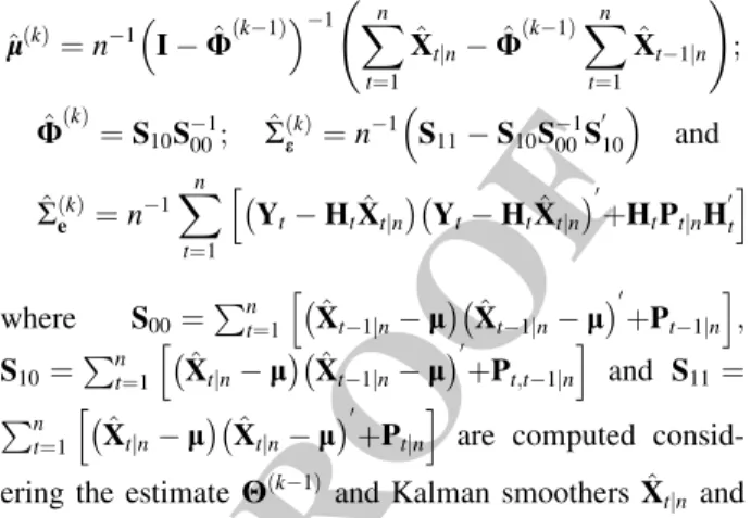
lð Þk ¼ n&1 I& ^Uðk&1Þ

# $&1 _Xn t¼1 ^ Xtjn& ^U k&1 ð ÞXn t¼1 ^ Xt&1jn ! ; ^ Uð Þk ¼ S10S&100; R^ k ð Þ e ¼ n &1 _S 11& S10S&100S 0 10 # $ and ^ Rð Þek ¼ n &1X n t¼1 Yt& HtX^tjn ! " Yt& HtX^tjn ! "0 þHtPtjnH 0 t h i 341 341 where S00¼ Pn t¼1 X^t&1jn& l ! " _^ Xt&1jn& l ! "0 þPt&1jn h i ; 342 S10¼ Pn t¼1 X^tjn& l ! " _^ Xt&1jn& l ! "0 þPt;t&1jn h i and S11¼ 343 Pn t¼1 X^tjn& l ! " _^ Xtjn& l ! "0 þPtjn h i

are computed consid-344 ering the estimate Hðk&1Þand Kalman smoothers ^Xtjnand

345 ^

Xt&1jnand its MSE, Shumway and Stoffer (1982).

346 Table2 shows parameters estimates (for the 16 water

347 monitoring sites in the study) obtained by gaussian

maxi-348 mum likelihood estimation by using EM algorithm, as

349 shown before. In the parameter estimation process, we

350 opted for replacing missing values with seasonal

coeffi-351 cient estimates, because a significant number of missing

352 values can difficult the convergence of parameter

estima-353 tion process. On the one hand, the global means estimates

354 indicate that monitoring sites Cantela˜es (CANT), Visela

355

Santo Adria˜o (VSA), Ferro (FER) and Gola˜es (GOL)

356 present the best water quality, considering the DO

con-357 centration. On the other hand, at monitoring sites Ponte

358 Branda˜o(PBR), Ponte Trofa (PTR), Santo Tirso (STI) and

359 Portos(POR) we obtained the lowest values means of DO

360 concentration, i.e., these locations have the worst water

361 quality. These conclusions are reinforced by the analysis of

362 error variances estimates. Indeed, low values of both

363 variances estimates, mainly the variance error estimates of

364 the state equation, are obtained at locations with high

365 means of DO concentration. If we consider the

geograph-366 ical locations corresponding to the lowest values of

vari-367 ance errors estimates, we conclude that DO has less

368 variability at water monitoring sites closer to the sources of

369 River Ave and its adjacent streams.

370 Residuals analysis was performed for each of the 16

371 monitoring sites in order to evaluate the models

adjust-372 ment. Globally, satisfactory fits were obtained in all

mon-373 itoring sites. Although some histograms indicate slightly

374 skewed residuals, the Smirnov–Kolmogorov test does not

375 reject the normal distribution of residuals in none of the

376 monitoring sites under study. In some monitoring sites, for

377 instance Ponte Trofa (PTR) and Portos (POR), PACF and

378 ACF plots seem to indicate the existence of a seasonal

379 component. However, as our main objective in this context

(6)

UNCORRECT

ED

PROOF

380 _{is to model the global behaviour to identify homogenous}

381 _{groups concerning DO magnitude, we thought that this}

382 _{aspect could be neglected at this moment, considering the} 383 _{gain in simplicity and parsimony of models.}

384 3.3 Discrepancy measure and clustering results

385 _{Adapting the discrepancy measure suggested in Bengtsson} 386 _{and Cavanaugh (}₂₀₀₈_{), we define a discrepancy measure} 387 _{based on the state component by considering the Kullback} 388 _{information (Kullback}₁₉₆₈_{) for the state densities f XjH}_ð _i_Þ 389 _{and f XjH}! _j" dX Yi; Hi;Hj ! " ¼ Eiln f Xð ijHiÞ f XijHj ! " ¼ Z lnf Xð ijHiÞ f XijHj ! "f XijYi;Hi ! "dX: ð5Þ 391

391 _{The pseudo-distance between two monitoring sites i and} 392 _{j, based on (}₅_{), defined as a form of the J-divergence} 393 _(Kullback₁₉₆₈_{), accounts for the different lengths of each} 394 _{series of data sets by averaging over time}

! JX Yi; Hi;Yj; Hj ! " ¼ N&1 i d X _Y i; Hi;Hj ! " þ N_j&1dX Yj; Hj;Hi ! ": 396

396 _{Employing output from the EM algorithm, including the} 397 _{maximum likelihood estimates, the sample !}_JX_-divergence

398 _{(Bengtsson and Cavanaugh}₂₀₀₈_{) reduces to} ! JX Yi; ^Hi;Yj; ^Hj # $ ¼ 1 2Nj^r2ei Sð Þ₁₁j & 2^/_iS₁₀ð Þj þ ^/2_iSð Þ₀₀j # $ þ 1 2Ni^r2ej Sð Þ₁₁i & 2j/S^ i ð Þ 10þ ^/ 2 jS ðiÞ 00 # $ & 1 400

400 _{where smoothing quantities S}ð Þk

11; S k ð Þ 10; S k ð Þ 00 and parameters

401 _{estimates ^}_H_k _{are computed based on the model Y}_ð _k_{; H}_k_Þ: 402 _{The defined symmetric J-divergence is based solely on} 403 _{the state process and targets only the state densities} 404 _{f X}_ð _i_jH_i_{Þ and f X}! _j_jH_j

"; where i and j are two water moni-405 _{toring sites and d}X _Y

i; Hi;Hj

!

" provides an unbiased esti-406 _{mate of the Kullback information between f X}_ð _i_jH_i_{Þ and} 407 _{f X}! _j_jH_j": The evaluation of the discrepancy measure solely 408 _{depends on the parameters estimates and on partial values} 409 _{obtained from the parameters estimation procedure} asso-410 _{ciated to each location’s model. Thus, as occurs in this case}

411 study, the data series does not necessarily have to be

412 reported over the same timeframe. However, the

applica-413 tion of any process of data series clustering relative to

414 contemporary periods should be accompanied by an

anal-415 ysis of the impact on results. The legitimacy of the

appli-416 cation of this procedure to these data series follows the fact

417 that data do not present an accentuated tendency nor

418 structural changes over time. Moreover, their magnitudes

419 are too small, even in the cases where linear models

indi-420 cate a statistical significant slope in the linear tendency (as

421 it is shown later); consequently, state space models can

422 accommodate this component through their known

versa-423 tility and dynamics.

424 By using the parameters estimates of Table1 and the

425 partial results of EM algorithm, the calculation of sample

426 values !JX Yi; ^Hi;Yj; ^Hj

# $

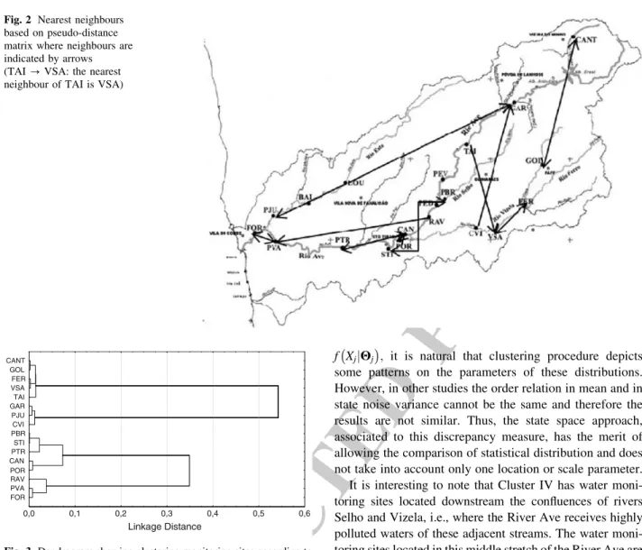
; i; j¼ 1; . . .16 allowed to obtain 427 a matrix of pseudo-distances. In Fig.2, nearest neighbours

428 are represented based on pseudo-distance matrices. It can

429 be seen from the plot that the location of each water

430 monitoring site in the river or its adjacent streams (closer to

431 the source of the river or to the confluence of the River Ave

432 with its adjacent streams) is an important factor to

deter-433 mine the nearest neighbour. However, the location of point

434 sources such as industries and domestic wastewater induces

435 some neighbour relations between Santo Tirso (STI) and

436 Ponte Branda˜o(PBR).

437 In order to identify potential clusters, we apply

clus-438 tering procedures by using the discrepancy matrix

pro-439 duced by evaluation of !JX Yi; ^Hi;Yj; ^Hj

# $

; i; j¼ 1; . . .16: 440 The discrepancy matrix was subjected to Ward’s, single

441 linkage and complete linkage clustering procedures

(Eve-442 ritt et al.2001). Because the three methods produce similar

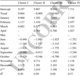
443 results, we only discussed the results of Ward’s method. As

444 seen in the dendrogram in Fig.3, the identified clusters are

445 given by sites: Cluster I {CANT, TAI, GOL, FER, VSA};

446 Cluster II {GAR, PJU, CVI}, Cluster III {RAV, PVA,

447 FOR} and Cluster IV {PBR, CAN, POR, STI, PTR}, which

448 are geographically represented in Fig.4.

449 Considering the estimates of the processes mean

450 obtained in the estimation procedure and indicated in

451 Table2, it is clear that the clustering procedure performs a

452 classification of the monitoring sites into a possible water

453 quality scale, in what concerns the annual mean DO

con-454 centration. In fact, the estimates of the processes mean in

Table 2 Gaussian maximum likelihood parameter estimates for the 16 water monitoring sites in the clustering process

Site CANT GAR TAI PBR RAV CAN POR STI PTR PVA FOR PJU GOL FER VSA CVI ^ l 10.017 9.256 9.427 7.240 8.166 8.286 7.843 7.609 7.439 8.457 8.034 9.016 9.642 9.672 9.809 9.357 ^ / 0.568 0.581 0.657 0.537 0.616 0.586 0.646 0.561 0.521 0.644 0.598 0.567 0.596 0.566 0.605 0.645 ^ r2 e 0.035 0.271 0.0005 2.199 0.002 0.616 2.203 0.003 0.020 0.194 0.010 0.033 0.008 0.004 0.003 0.002 ^ r2 e 0.724 1.381 0.780 4.184 2.055 3.136 3.340 4.210 3.517 2.489 2.718 1.240 0.752 0.832 0.825 1.366

Author Proof

(7)

UNCORRECT

ED

PROOF

455 _{Cluster I monitoring sites present the highest values}

456 _{obtained from the DO concentration. Indeed, the five}

457 monitoring sites of Cluster I present the best water quality 458 annual indicators, while the worst indicators are observed

459 _{in Cluster IV monitoring sites. On the one hand this}

460 _{methodology allows classifying the water monitoring sites,} 461 _{in regard to annual mean DO concentration, in four} cate-462 _{gories: from best water quality (Cluster I) to worst water} 463 _{quality (Cluster IV). On the other hand, clustering} proce-464 _{dure performs a discrimination of water monitoring sites} 465 _{based on state noise variance. Indeed, Cluster I corresponds} 466 _{to locations with the lowest state noise variances; Cluster II} 467 _{has state noise variances greater than Cluster I and so on.} 468 _{As expected, similar results are not obtained by observing} 469 equation variance because the J-divergence !JX Yi; ^Hi;

#

470 Yj; ^HjÞ is based on the state process. Since the discrepancy

471 _{measure tends to compare state densities f X}_ð _i_jH_i_{Þ and}

472 f XjjHj

!

"; it is natural that clustering procedure depicts 473 some patterns on the parameters of these distributions.

474 However, in other studies the order relation in mean and in

475 state noise variance cannot be the same and therefore the

476 results are not similar. Thus, the state space approach,

477 associated to this discrepancy measure, has the merit of

478 allowing the comparison of statistical distribution and does

479 not take into account only one location or scale parameter.

480 It is interesting to note that Cluster IV has water

moni-481 toring sites located downstream the confluences of rivers

482 Selho and Vizela, i.e., where the River Ave receives highly

483 polluted waters of these adjacent streams. The water

moni-484 toring sites located in this middle stretch of the River Ave are

485 much more polluted, probably because they are close to

486 densely populated areas with high industrial production units.

487 4 Forecasting models

488 As mentioned above, data not considered in the modelling

489 process was used in the assessment of the performance of

490 the adjustment models: LM and state space models,

con-491 sidering the obtained clustering results concerning the

492 mean square error forecast. Thus, for each of the four

493 clusters identified in last section, two models are

estab-494 lished by using the available data until September 2006.

495 As we considered that inside each cluster there is a

496 homogenous annual mean behaviour of DO, it is

reason-497 able to assume that monthly measurements of water

mon-498 itoring sites inside a cluster are observations of the same

499 process. Therefore, models have to accommodate

repli-500 cates at each time. Moreover, as the goal at this stage is to

Fig. 2 Nearest neighbours based on pseudo-distance matrix where neighbours are indicated by arrows (TAI ? VSA: the nearest neighbour of TAI is VSA)

FOR PVA RAV POR CAN PTR STI PBR CVI PJU GAR TAI VSA CANT FER GOL 0,0 Linkage Distance 0,1 0,2 0,3 0,4 0,5 0,6

Fig. 3 Dendrogram showing clustering monitoring sites according to DO characteristics based on Ward’s method

(8)

UNCORRECT

ED

PROOF

501 _{make monthly predictions of the DO concentration, the} 502 _{seasonality component should not be omitted in models} 503 _{formulations.}

504 _{4.1 Linear models}

505 _{This section presents the linear models used to describe the} 506 _{main characteristics of the DO series and to adjust different} 507 _{models to each homogeneous group of monitoring sites} 508 _{(cluster). Linear models are primary tools in the context of} 509 _{environmental problems. There are many contributions} 510 _{(Carl and Ku¨hn} ₂₀₀₈_{; Mourin˜o and Bara˜o}₂₀₀₉_; Paschal-511 _{idou et al.}₂₀₀₉_{). Linear models are simple and have good} 512 _{statistical properties; they are very robust statistical} meth-513 _{ods and this feature makes them a very attractive} frame-514 _{work to describe the quality variables under study. It is} 515 _{well known that the choice of the independent variables} 516 should rely on the principle of parsimony. Also, their 517 selection is heavily context dependent, because both vari-518 _{ables themselves and the respective estimates for the} 519 _{coefficients should have a clear interpretation within the} 520 _{framework in which the case study is included.}

521 _{Environmental data are naturally affected by the} dif-522 _{ferent seasons and by the environmental degradation that} 523 _{has been verified in a more aggravated way in recent years.} 524 _{Thus, any model to predict the behaviour of data must take} 525 _{these two factors into account. In this case study there is no} 526 _{measure of space continuity and, therefore, the} observa-527 _{tions at different locations in the cluster will be treated as} 528 independent observations, referenced in time. Hence, 529 within each cluster we consider a variable observation 530 _{by Y}ð Þi

j;t; where i represents the cluster, i = 1, 2, 3, 4,

531 jrepresents the monitoring site running along all the sites

532 in the cluster i, j¼ 1; . . .; ki and t¼ 1; . . .; nðiÞj stands for

533 the month. With this notation, the model in each cluster

534 i includes two additive components corresponding to

dif-535 ferent types of effects, that is,

Y_j;tð Þi ¼ Ttð Þi þ S i ð Þ t þ e i ð Þ j;t: ð6Þ 537 537 Let us now analyse in more detail how to describe each

538 component with the help of a linear model. The trend is

539 generally described by a simple linear function of time,

540 Ttð Þi ¼ að Þi þ bð Þit: The seasonal component S

i ð Þ t is a

541 periodic function taking 12 different values, say, kð Þ_si;

542 s = 1,…, 12 associated with each month of the year and

543 expressing the positive or negative deviation from the trend

544 due to the effect of that month. This type of effect is

545 usually described with the help of 12 dummy variables

546 indicating if each time instant t corresponds to month

547 i. However, when the model has a constant term, in order

548 for these parameters to be estimable they have to add up to

549 0, that is,P12 s¼1ks¼ 0 and kð Þ12i ¼ & P11 s¼1k i ð Þ s : Thus, as one 550 of the seasonal coefficients has to be written as a function

551 of the others, the seasonal component is represented by a

552 linear combination of 11 explanatory variables

SðiÞt ¼

X11

s¼1

kð Þ_siSs;t;

where Ss;t¼

1; if date t corresponds to month s &1; if date t corresponds to month 12

0; otherwise 8 < : : 554 554 Clearly, the choice of the twelfth month, December, to

555 be written as a linear combination of the others is arbitrary

Fig. 4 Representation of clusters in the River Ave hydrological basin

(9)

UNCORRECT

ED

PROOF

556 _{and any month can be used for that role. Finally, the model} 557 _{includes a stochastic component, e}ð Þi

j;t; which we suppose to

558 _{be simply a white noise process, that is, a sequence of} 559 _{uncorrelated zero mean random variables, with constant} 560 _{variance r}2 ið Þ_{: A careful check of residuals shows that there}

561 _{were no significant violations of the normality and}

562 _{independence conditions. This procedure ensures the}

563 optimality properties of the OLS as well as the power of 564 _{the t and F tests performed. After the model with all} 565 _{variables (full model) was adjusted, the authors used a} 566 _{backwards elimination procedure to select the significant} 567 _{variables. The regressor with largest p-value for its} 568 _{t-statistic was removed at each step, until all the regressors} 569 _{were significant at the level 0.05. The final reduced model} 570 _{was also tested against the full model with the help of a} 571 _{F-test on the set of all removed independent variables.} 572 _{The DO modelling procedure starts by fitting the linear} 573 _{model (}₆_{) to the DO data observed in each cluster. The} 574 _{regression parameters obtained for each cluster are} pre-575 sented in Table3. As expected, the four clusters show a 576 _{seasonal pattern with lower values of DO concentration in}

577 _{the warmer months as compared to autumn and winter}

578 _{months. This could be expected because the inverse} rela-579 _{tionship between temperature and DO is a natural} pro-580 _{cess—warmer water becomes more easily saturated with} 581 _{oxygen and it can hold less DO. Cluster I presents a weak} 582 _{positive significant trend associated to the sites in rural} 583 _{areas near the source of the river with good water quality.} 584 _{Cluster II and Cluster III present a weak decreasing trend} 585 _{associated to polluted areas that are densely populated,} 586 _{with high industrial productivity and where the Ave also}

587 receives similarly polluted waters from its adjacent

588 streams. Cluster III presents the highest coefficient of

589 determination (69%). Cluster IV, the most polluted cluster,

590 has a stable behaviour with no significant trend, which may

591 be justified if we take into consideration the highest

vari-592 ability when compared with other clusters. In this case, the

593 coefficient of determination was 57%.

594 4.2 State space models

595 In the previous section it was verified that the seasonality is

596 an important structural component to predict the monthly

597 DO concentration. Thus, a regression model with varying

598 coefficients (Pagan1980; Leybourne2006) represented in a

599 state space framework could improve the predictions

600 accuracy. However, in this case it implies establishing

601 multivariate models that involve a large number of

602 parameters, in addition to a complex structure that

diffic-603 ults its interpretation.

604 We propose an alternative model that assumes prior

605 knowledge of DO seasonal coefficients st or its estimates

606 (in this case, its monthly means computed in the past). This

607 assumption implies some knowledge of the seasonal

608 component behaviour. However, the modelling of this type

609 of data is usually performed under previous studies or

610 considering a significant data set. Another solution to

611 overcome the monthly means of DO could be the use of

612 seasonal coefficients estimates obtained via the linear

613 process. Nevertheless, we selected the simplest option to

614 compute the monthly means of observations, to compare

615 linear regression with state space approaches in order to

616 guarantee the independency of two estimation processes.

617 The model assumes that for month t the measurement

618 Y_j;tð Þi of the DO in monitoring site j of the cluster i is the

619 calibrated seasonal coefficient added to a zero mean error,

620 i.e., Y_j;tð Þi ¼ sð Þtibð Þti þ e

i ð Þ

j;t; where bð Þti is a calibration factor of

621 cluster i at time t. Considering that cluster i is composed by

622 ki water monitoring sites, the DO can be modelled at

623 cluster i by Yð Þti ¼ s i ð Þ t bð Þti þ e i ð Þ t : ð7Þ 625 625 bð Þ_ti & 1 ¼ /ð Þi _bð Þi t&1& 1 # $ þ eð Þti: ð8Þ 627 627 where Yð Þti ¼ Y i ð Þ 1;t; Y i ð Þ 2;t; . . .; Y i ð Þ ki;t h i0 and sð Þti ¼ s i ð Þ t ! 1ki: The 628 error vector eð Þti ¼ e i ð Þ 1;t; e i ð Þ 2;t; . . .; e i ð Þ ki;t h i0

and the error eð Þti are

629 zero means uncorrelated errors, E eð Þ_j;tieð Þi

s

h i

¼ 0 for all t, 630 sand j, with matrix of covariance E eð Þtie

0_{ð Þ}_i t h i ¼ r2 e;i! Ikiand 631 variance E e2 t;i h i ¼ r2

e;i; respectively. The calibration factor

632 bð Þ_ti is assumed to be a stationary autoregressive process of

633 order 1, /ðiÞ ' ' ' ' '

'\1; with unitary mean.

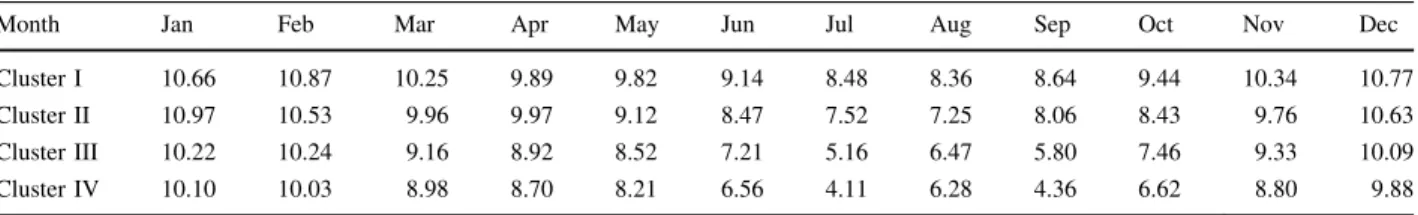
Table 3 Results for linear models adjustment to the four clusters Cluster I Cluster II Cluster III Cluster IV Intercept 9.197 9.867 8.634 7.711 Trend 0.004 -0.009 -0.003 – January 0.960 1.382 2.045 2.540 February 1.117 1.410 2.122 2.457 March 0.602 0.577 0.983 1.323 April – 0.784 0.708 1.027 May – – – – June -0.440 -1.093 -1.025 -1.352 July -1.160 -1.557 -3.143 -3.391 August -1.426 -2.037 -1.755 -1.501 September -0.980 -0.912 -2.441 -3.240 October -0.520 -0.546 -0.780 -1.143 November 0.720 0.711 1.183 1.118 December 1.125 1.281 2.103 2.161 ^ r2ðiÞ _0.854 _1.019 _1.198 _1.766 R2 0.50 0.58 0.69 0.57

Author Proof

(10)

UNCORRECT

ED

PROOF

634 _Table₄ _{summarizes seasonal coefficients estimates for} 635 _{the four clusters computed by the mean of the observed} 636 _{values of the DO concerning monitoring sites that belong} 637 _{to each cluster and according each month. Table}₅_presents

638 _{gaussian maximum likelihood estimates of parameters}

639 _{(referred in Sect. 3.2) that concern each cluster’s} multi-640 _{variate model (}₇_)–(₈_{). As mentioned before, the state} 641 _{process b}ð Þi

t can be interpreted as a dynamic calibration

642 factor of the seasonal component; so, it is reasonable that 643 _{state noise has a small variance, as can be seen in Table}₅_. 644 _{The largest values of both state and observation equations} 645 _{error variances are obtained in Clusters III and IV. As} 646 _{mentioned before concerning the clustering analysis, these} 647 _{clusters include the water monitoring sites which have the} 648 _{lowest annual DO values. Therefore, Clusters III and IV} 649 _{include sites with worse indicators in what concerns DO} 650 _{concentration, but at the same time they also present the} 651 _{largest variability. Nevertheless, Cluster IV presents worse} 652 _{water quality indicators that clearly distinguish it, even} 653 _{from Cluster III.}

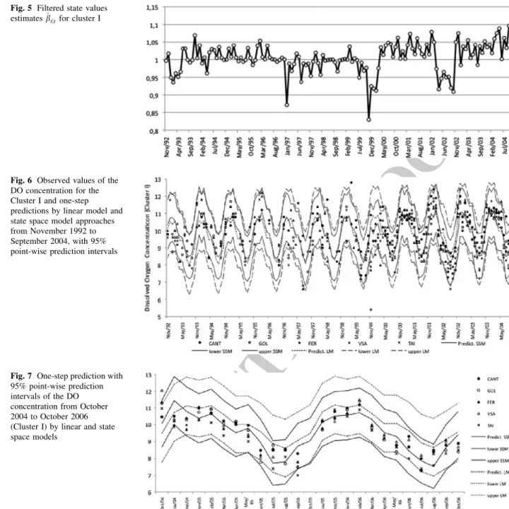
654 Taking advantage of the interpretability of the state 655 _{process, Fig.}₅ _{shows filtered state values estimates ^}_b

tjt in

656 _{the modelling period. As the graphic shows, the model}

657 _{captures changes in a dynamic way that overlaps the}

658 _{default behaviour evidenced by the seasonality. The state} 659 _{space model (}₇_)–(₈_{) provides a useful tool to evaluate} 660 _{changes in real time on DO concentration in each month.} 661 _{Indeed, calibration factor estimates greater than one} indi-662 _{cate an improvement in water quality, while estimates} 663 _{lower than one can indicate water quality deterioration.} 664 _{This possibility of model formulation (}₇_)–(₈_{) benefits the} 665 _{water monitoring process in a way that linear models are} 666 not able to provide, since linear models incorporate global 667 trends in pre-established time periods.

668 4.3 Comparative analysis

669 A first analysis of adjustment models is done comparing

670 data and predictions. Globally, models fit the data

satis-671 factorily. For instance, Fig. 6 shows the observed values

672 and one-step predictions of the DO concentration

con-673 cerning Cluster I from November 1992 to September 2004,

674 with 95% point-wise prediction intervals. Graphic

repre-675 sentation shows that the linear model produces point-wise

676 prediction intervals with large amplitude than state space

677 models, as is the case in other clusters. As the state space

678 model incorporates the last observation at each time, it

679 enables updating and accurate predictions.

680 Accurate forecasts are important information on water

681 monitoring processes; therefore, they are a good criterion to

682 assess the model performance. Thus, we compare the linear

683 and state space models performance concerning the one-step

684 forecast’s mean square error, relatively to the remaining

685 unused data in the modelling process. So, we computed

686 forecasts for the 228 observations by using two approaches.

687 However, approximately half of this data is related to Cluster

688 I, because some water monitoring sites belonging to other

689 clusters were inactive due to public policy restructuring.

690 In order to compute forecasts based on linear models, we

691 applied the estimated regression equation obtained from

692 Table3, while state space models forecasts are evaluated

693 through Kalman filter predictors. The Kalman filter

algo-694 rithm produces the best linear prediction ^bð Þ_tjt&1i for the

cali-695 bration factor bð Þ_ti for month t and cluster i and,

696 consequently, the best linear prediction of DO is ^Ytð Þi ¼

697 sð Þtib^

i ð Þ

tjt; which is clearly equal for all sites from a same cluster

698 at each month.

699 In Fig.7 we present forecasts with 95% point-wise

700 prediction intervals of DO concentration from October

701 2004 to October 2006. We do not have records from

702 October 2005 in any of the water monitoring sites and we

703 were not able to determine the cause of this occurrence.

704 This representation indicates that state space approach

705 allows obtaining prediction intervals with lower range than

706 linear models. The state space model tends to fit data

707 better, whereas the linear model seems to overestimate the

708 values. In this concrete cluster, the linear model considers

709 the trend as a significant component with a small positive

710 slope in the modelling period. Nevertheless, its rigid

Table 4 Seasonal coefficients (monthly means) of the DO concentration of the four clusters

Month Jan Feb Mar Apr May Jun Jul Aug Sep Oct Nov Dec

Cluster I 10.66 10.87 10.25 9.89 9.82 9.14 8.48 8.36 8.64 9.44 10.34 10.77 Cluster II 10.97 10.53 9.96 9.97 9.12 8.47 7.52 7.25 8.06 8.43 9.76 10.63 Cluster III 10.22 10.24 9.16 8.92 8.52 7.21 5.16 6.47 5.80 7.46 9.33 10.09 Cluster IV 10.10 10.03 8.98 8.70 8.21 6.56 4.11 6.28 4.36 6.62 8.80 9.88

Table 5 Estimated values obtained for the multivariate models parameters of the four clusters via gaussian maximum likelihood estimation Cluster /^ ^r2 e r^2e I 0.5213 0.0016 0.3140 II 0.5246 0.0035 0.5549 III 0.7527 0.0036 0.7138 IV 0.2242 0.0158 1.6322

Author Proof

(11)

UNCORRECT

ED

PROOF

711 _{structure may not have detected temporary changes or new} 712 _{conditions such as new industries in that area, for instance.} 713 _{In order to compare the two approaches in a} quantita-714 _{tively point of view, in the sense of predictions accuracy,} 715 _{we computed the root of the mean square errors (RMSE) of} 716 _{predictions, i.e.,} RMSE¼ ffiffiffiffiffiffiffiffiffiffiffiffiffiffiffiffiffiffiffiffiffiffiffiffiffiffiffiffiffiffiffiffiffiffiffiffiffiffiffiffiffiffiffiffiffiffiffiffiffiffiffi 1 228 X4 i¼1 Xni t¼1 Ytð Þi & ^Y i ð Þ t # $2 v u u t : 718

718 _{Taking into account all 228 predictions computed}

719 _{in the period of the assessment procedure, we obtained}

720 RMSE = 0.961 in the linear models and RMSE = 0.846

721 in the state space approach. Globally, it is the state space

722 modelling approach that provides the least RMSE as far as

723 concerns all the predictions we made. So, the dynamic

724 structure of the state space models improved the

725 predictions accuracy in the sense of the mean square error.

726 5 Conclusions

727 This work shows that state space approach combined with

728 clustering techniques allows identifying homogeneous

Fig. 5 Filtered state values estimates ^b_tjtfor cluster I

Fig. 6 Observed values of the DO concentration for the Cluster I and one-step predictions by linear model and state space model approaches from November 1992 to September 2004, with 95% point-wise prediction intervals

Fig. 7 One-step prediction with 95% point-wise prediction intervals of the DO concentration from October 2004 to October 2006 (Cluster I) by linear and state space models

(12)

UNCORRECT

ED

PROOF

729 _{groups of water monitoring sites, based on similarities in}

730 _{the temporal dynamics of monthly records of DO}

con-731 _{centration. With an appropriate disparity measure based} 732 _{on Kullback information, we identified four clusters of} 733 _{water monitoring sites in the River Ave basin that allow} 734 _{us to construct only four models in order to forecast this} 735 _{variable in the future by reducing the initial 16 water} 736 monitoring sites. Besides, it is possible to arrange these 737 _{groups by order of water quality degree, from the less} 738 _{polluted (Cluster I) to the most polluted (Cluster IV). So,} 739 _{the less polluted monitoring sites are near the sources of} 740 _{River Ave or its adjacent streams (except for river Selho),} 741 _{and the most polluted water monitoring sites are located}

742 _{in a highly industrial area exposed to discharges of}

743 _{industrial effluents.}

744 _{After a clustering procedure, the comparison between}

745 _{the forecast’s mean square error of the linear model and} 746 _{of the state space model shows that the latter evidences an} 747 _{improved accuracy within the proposed assessment}

per-748 iod. We adopted a state space model to predict the

749 _{monthly DO concentration, which calibrates the seasonal} 750 _{coefficients through an autoregressive calibration factor.} 751 _{This approach is an alternative to the standard linear}

752 _model _with _tendency _and _seasonality _components,

753 _{because this model incorporates a dynamic structure that} 754 _{allows an easy data fitting. Furthermore, calibration} fac-755 _{tors have a useful interpretation as an approximate ratio}

756 _{between observed measure of the DO concentration and}

757 _{the respective seasonal coefficient. This approach} pro-758 _{vides a real time procedure to monitoring DO} concen-759 _{tration in which calibration factors greater or lower than} 760 one indicate that water quality improved or deteriorated in 761 _{comparison to the expected value based on past} behav-762 _{iour. From the forecast point of view, the state space}

763 _{model reduced the forecast’s mean square error from}

764 _{0.961 (obtained with linear model) to 0.846, which is a} 765 _{significant improvement.}

766 _{We hope that this work could be a tool for decision}

767 _{support, because monitoring procedures and good models} 768 _{of water quality variables are indispensable, mainly in a} 769 _{highly industrial region as is the Ave Valley in the} north-770 _{west of Portugal.}

771 _{Acknowledgments} _{The authors would like to thank the anonymous} 772 _{referees for many helpful critics and suggestions that contributed to} 773 _{improve this paper. The authors would like to thank to Eng. Pimenta} 774 _{Machado from the Portuguese Regional Directory for the Northern} 775 _{Environment and Natural Resources and to Eng. Claúdia Brandaõ} 776 _{from the Portuguese Institute of Water, for sharing their skills and} 777 _{experiences and for supplying the monitored data. A. Manuela} 778 _{Gonçalves acknowledges the financial support provided by the} 779 _{Research Centre of Mathematics of the University of Minho through} 780 _{the FCT Pluriannual Funding Program.}

781 References

782

Alpuim T, Barbosa S (1999) The Kalman filter in the estimation of

783

area precipitation. Environmetrics 10:377–394

784

Bengtsson T, Cavanaugh JE (2008) State-space discrimination and

785

clustering of atmospheric time series data based on Kullback

786

information measures. Environmetrics 19:103–121

787

Boi P (2004) A statistical method for forecasting extreme daily

788

temperatures using ECMWF 2-m temperatures and ground

789

station measurements. Meteorol Appl 11:245–251

790

Brown P, Diggle P, Lord M, Young P (2001) Space-time calibration

791

of radar rainfall data. Appl Stat 50(2):221–241

792

Carl G, Ku¨hn I (2008) Analysing spatial ecological data using linear

793

regression and wavelet analysis. Stoch Environ Res Risk Assess

794

22(3):315–324

795

Costa M, Alpuim T (2010) Parameter estimation of state space

796

models for univariate observations. J Stat Plan Inference

797

140(7):1889–1902

798

Dempster AP, Laird NM, Rubin DB (1977) Maximum likelihood

799

from incomplete data via the EM algorithm. J R Stat Soc Ser B

800

39:1–38

801

Everitt BS, Landau S, Leese M (2001) Cluster analysis, 4th edn.

802

Arnold, London

803

Fovell R, Fovell M (1993) Climate zones of the conterminous United

804

States defined using cluster analysis. J Clim 6:2103–2135

805

Galanis G, Anadranistakis M (2002) A one-dimensional Kalman filter

806

for the correction of near surface temperature forecast. Meteorol

807

Appl 9:437–441

808

Gong X, Richman M (1995) On the application of cluster analysis to

809

growing season precipitation data in North America east of the

810

Rockies. J Clim 8:897–931

811

Harvey AC (1996) Forecasting structural time series models and the

812

Kalman filter. Cambridge University Press, Cambridge

813

Kullback S (1968) Information theory and statistics. Dover, New York

814

Leybourne SJ (2006) Estimation and testing of time-varying

coeffi-815

cient regression models in the presence of linear restrictions.

816

J Forecast 12(1):49–62

817

Libonati R, Trigo I, DaCamara C (2008) Correction of 2

m-818

temperature forecasts using Kalman filtering technique. Atmos

819

Res 87:183–197

820

Mourin˜o H, Bara˜o MI (2009) A comparison between the linear

821

regression model with autocorrelated errors and the partial

822

adjustment model. Stoch Environ Res Risk Assess 24(4):

823

499–511

824

Oliveira RES, Lima MMCL, Vieira JMP (2005) An indicator system

825

for surface water quality in river basins. In: Inter-Celti colloquium

826

on hydrology and management of water resources 4, Guimara˜es

827

Pagan A (1980) Some identification and estimation results for

828

regression models with stochastically varying coefficients.

829

J Econom 13:341–363

830

Paschalidou AK, Kassomenos PA, Bartzokas A (2009) A comparative

831

study on various statistical techniques predicting ozone

concen-832

trations: implications to environmental management. Environ

833

Monit Assess 148:277–289

834

PGIRH/N (1988) Metodologias para a Avaliac¸a˜o de Polı´ticas de

835

Recursos Hı´dricos - Plano de Gesta˜o da Bacia Hidrogra´fica do

836

Rio Ave (in Portuguese). Ministe´rio das Obras Pu´blicas,

837

Transportes e Comunicac¸o˜es, Laborato´rio Nacional de

Enge-838

nharia Civil, Ministe´rio do Plano e Administrac¸a˜o do Territo´rio,

839

Comissaõ de Coordenaçaõ da Regiaõ Norte 8:66, Lisboa

840

PGIRH/N and NATO PO-RIVERS (1994) Caracterizac¸a˜o e

Direct-841

rizes de Planeamento dos Recursos Hı´dricos do Norte – A Bacia

842

Hidrogra´fica do Rio Ave (in Portuguese). Ministe´rio do

(13)

UNCORRECT

ED

PROOF

843 _{Ambiente e dos Recursos Naturais, Direcc¸a˜o Regional do} 844 _{Ambiente e Recursos Naturais, Instituto da A}_{´ gua. Porto 1–5,}

845 _1–13

846 _{Shrestha S, Kazama F (2007) Assessment of surface water quality} 847 _{using multivariate statistical techniques: a case study of the Fuji} 848 _{river basin, Japan. Environ Model Softw 22:464–475}

849 _{Shumway R, Stoffer D (1982) An approach to time series smoothing} 850 _{and forecasting using the EM algorithm. J Time Ser Anal} 851 _3:253–264

852

Shumway R, Stoffer D (2006) Time series analysis and its

applica-853

tions, 2nd edn. Springer-Verlag, Berlin

854

Stone RC (1989) Weather types at Brisbane, Queensland: an example

855

of the use of principal components and cluster analysis. Int J

856

Climatol 9:3–32

857