POLYNOMIAL CHAOS EXPANSION FOR GENERAL MULTIVARIATE DISTRIBUTIONS WITH CORRELATED
VARIABLES
MARIA NAVARRO, JEROEN WITTEVEEN, JOKE BLOM⋆
Abstract. Recently, the use of Polynomial Chaos Expansion (PCE) has been in-creasing to study the uncertainty in mathematical models for a wide range of appli-cations and several extensions of the original PCE technique have been developed to deal with some of its limitations. But as of to date PCE methods still have the restriction that the random variables have to be statistically independent. This paper presents a method to construct a basis of the probability space of orthogonal poly-nomials for general multivariate distributions with correlations between the random input variables. We show that, as for the current PCE methods, the statistics like mean, variance and Sobol’ indices can be obtained at no significant extra postprocess-ing costs. We study the behavior of the proposed method for a range of correlation coefficients for an ODE with model parameters that follow a bivariate normal dis-tribution. In all cases the convergence rate of the proposed method is analogous to that for the independent case. Finally, we show, for a canonical enzymatic reaction, how to propagate experimental errors through the process of fitting parameters to a probabilistic distribution of the quantities of interest, and we demonstrate the signif-icant difference in the results assuming independence or full correlation compared to taking into account the true correlation.
Keywords. Uncertainty quantification ⋆ polynomial chaos expansion ⋆ correlated
inputs
CWI, Science Park 123, 1098 XG Amsterdam, the Netherlands ⋆Corresponding author. Tel.:+31 205924263
Email addresses. [email protected], [email protected], [email protected]
1. Introduction
To describe real-life phenomena we often make use of deterministic mathematical mod-els. Typical constituents of such models are assigned a definite value and we seek a deterministic solution to the problem. In reality, however, those phenomena will al-most always have uncertain components: unknown parameters, imprecise experimental data, etc.. A precise mathematical description should reflect such uncertainties. In other words, the parameters of a mathematical model of a real-life problem possess
Date: June 23, 2014.
1
randomness with, most likely, some degree of correlation between them as well. In studying the propagation of the uncertainty through the model and its effect on the final solution the great majority of the current techniques usually ignores the correla-tions between random inputs.
The simplest approach to study the model uncertainty is to apply a Monte Carlo sam-pling [1], where - once a probability density function (pdf) for the random inputs is assumed based on the a priori knowledge about them - the mean and other character-istics can be estimated from the output distribution, by sampling repeatedly from the assumed probability density function and simulating the model for each sample. Al-though with this approach it is possible to consider the correlations between variables, it yields reasonable results only if the number of samples is quite large, requiring a great computational effort. Moreover, the order of convergence is merely√N, whereN is the number of samples. To decrease the computational effort, several modifications lead-ing to new methods were introduced: Latin hypercube sampllead-ing [17], the Quasi-Monte Carlo (QMC) method [8], the Markov Chain Monte Carlo method (MCMC) [19], the Response Surface method (RSM) [26], etc.. Alternatively, deterministic methods to study parameter sensitivity have also been developed, e.g., perturbation methods[13], local expansion-based methods like Taylor series, and so on.
apply PCE when the inputs are linearly correlated, some methods have been proposed: linear transformations [22, 27], K-L expansion [16] or proper orthogonal decomposition [18]. All of these fix the problem by applying transformations to remove the corre-lations, which increases the complexity of the problem and degrades the convergence rate because of increased nonlinearity [7].
In this paper, we propose a - more fundamental - solution for the latter of those limitations, since correlations can have strong dynamical effects on the final solution as we will also show. We present a method to construct an orthogonal polynomial basis for any general multivariate distribution, including those with correlated random variables.
The outline of this paper is as follows: In Section 2 the extension is presented of the polynomial chaos expansion to general multivariate distributions and the derivation of the statistics of the Quantities of Interest (QoI) - like mean, variance, and Sobol’ indices - is discussed. In Section 3 we show for an ODE dependent on a bivariate normal distribution the effect of the strength of the correlation - from uncorrelated to fully correlated - on the solution. We also show that in all these cases the convergence rate for increasing expansion order is the same, i.e., the proposed method shows the same favourable convergence rate as the original PC method for an uncorrelated multivariate normal distribution. We then apply the method on a simple but realistic example from biochemistry, viz. the canonical enzymatic reaction [3], that has been used in a previous paper [2] to display the effect of noisy data on the reliability of the estimated parameters. We show thattruepropagation of the uncertainty in the parameters - i.e., including the correlation - effects the uncertainty in the QoI, the concentration of the product, significantly. Section 4 contains a discussion and concluding remarks.
2. PCE for multivariate arbitrarily distributed input variables
In this section we extend the polynomial chaos expansion for arbitrarily distributed independentrandom variables to themultivariatearbitrarily distributed PC expansion.
2.1. Polynomial chaos expansion. Consider the following stochastic equation in the probability space (Ω,A, P) where Ω is the event space, A ⊆ 2Ω
itsσ-algebra and
P its probability measure
(1) L(x,ξ(ω);u) = f(x,ξ(ω)), x∈X and ω∈Ω,
parameters or initial and boundary conditions. In order to make the notation less cumbersome, we denote the realization of a random vectorξ(ω), for ω ∈Ω, byξ∈Ξ, with Ξ the support of the pdf.
In the polynomial chaos method the random input ξ and the solution uare expanded into a series of polynomials
ξ =
∞
X
i=0
ξiΦi(ξ)
u(x,ξ) =
∞
X
i=0
ui(x)Φi(ξ),
(2)
separating the deterministic and the random variables. The Φi(ξ) are n-dimensional
polynomials that are mutually orthogonal with respect to the probability density func-tion ρ(ξ)
(3) hΦi(ξ),Φj(ξ)i=
Z
Ξ
Φi(ξ)Φj(ξ)ρ(ξ)dξ=||Φi||2δij,
with δij the Kronecker delta and||Φi||2 =hΦi,Φii. For independent random variables
the Φi’s are tensor products of one-dimensional polynomials, Φi(ξ) =
Qn
j=1Φ˜ji(ξj).
To determine the polynomial chaos expansion coefficients ξi and ui(x) there are two
main-stream methods, viz. Spectral Projection and Galerkin. Both project onto the polynomial space, but whereas in the spectral projection approach the expansion (2) is projected, in the Galerkin approach thegoverning equation (1), with the expansion substituted, is projected onto the polynomial space. Typically, for the random input variables the first approach is chosen, resulting in
(4) ξj = hξ,Φj(ξ)i hΦj(ξ),Φj(ξ)i
= 1 ||Φj||2
Z
Ξ
ξΦj(ξ)ρ(ξ) dξ, j = 0,1, ... .
If the function is truely nonlinear aliasing is a threat for the accuracy [40], therefore we will use the Galerkin method to obtain the solution. The expansions (2) are substituted into the stochastic equation (1) before being projected
*
L x,
∞
X
i=0
ξiΦi(ξ); ∞
X
i=0
ui(x)Φi(ξ)
!
,Φj(ξ)
+
=
=
*
f x,
∞
X
i=0
ξiΦi(ξ)
!
,Φj(ξ)
+
, j = 0,1, ... .
(5)
In practice, the number of expansion terms is truncated to
(6) (N+ 1) = (n+p)!
where pis the highest order of the polynomials and the integrals are either computed exactly or approximated using quadrature rules or Monte Carlo sampling. E.g., for a system of ODEs the differential operator in the left-hand side of (1) reduces to ˙u(t,ξ) and its projection onto Φj to ˙uj(t)||Φj||2.
2.2. Multivariate arbitrarily distributed input variables. In [39] a method has been proposed to extend the polynomial chaos method to an arbitrarily distributed univariate distribution. The one-dimensional polynomials Φi(ξ) are constructed to be
mutual orthogonal with respect to an arbitrarily pdf ρ(ξ) using the well-known and robust Gram-Schmidt orthogonalization method (see e.g. [10]). This method can be extended to multivariateindependent random variables, where the orthogonal multidi-mensional polynomials are the product of the constructed one-dimultidi-mensional orthogonal polynomials. Here we use the same orthogonalization approach to construct directly a multidimensional orthogonal polynomial basis, {Φj(ξ)}Nj=0, for correlatedmultivariate
random input variables. Since the Gram-Schmidt method constructs from an arbitrary basis a basis that is orthogonal with respect to a given innerproduct, the first step is the choice of a suitable set of linearly independent polynomials. It should be noticed that any linearly independent set of polynomials can be used in this method, but for simplicity we will use the set of monic polynomials{ej(ξ)}Nj=0 given by
(7) ej(ξ) = n
Y
l=1
ξjl
l , j = 0, . . . , N, jl∈ {0, . . . , p}, and n
X
l=1
jl ≤p,
where n is the dimension of the random vector ξ, p the highest polynomial degree chosen, and N + 1 the dimension of the polynomial basis given by Equation (6). E.g., if n = p = 2 then N + 1 = 6 and the set of linearly independent polynomi-als {ej(ξ1, ξ2)}j5=0 equals {1, ξ1, ξ2, ξ12, ξ
2
2, ξ1ξ2}. Next, the orthogonal polynomial basis
{Φj(ξ)}Nj=0 is constructed from {ej(ξ)}Nj=0 using the Gram Schmidt algorithm
Φ0(ξ) = 1,
Φj(ξ) = ej(ξ)− j−1
X
k=0
cjkΦk(ξ) for 1≤j ≤N,
(8)
where the coefficients cjk are given by
(9) cjk = h
ej(ξ),Φk(ξ)i
hΦk(ξ),Φk(ξ)i
Since each polynomial of the orthogonal basis {Φj(ξ)}Nj=0 can be written as a sum of
the monic polynomials ej(ξ), the inner products in Equation (9) can be calculated as
sum of raw moments
(10) µr1···rn
ξ =
Z
Ξ n
Y
l=1
ξrl
l ρ(ξ)dξ, rl ∈ {0, . . . ,2p}, and n
X
l=1
rl ≤2p.
With this procedure we immediately get a set of multidimensional orthogonal poly-nomials. Note, that if the random variables are independent these polynomials are the same as the ones obtained by taking the tensor-products of the one-dimensional orthogonal polynomials. Once these multidimensional orthogonal polynomials have been computed the PCE method can be applied analogously to the independent case, i.e., projection onto the polynomial space of either the expansion or the equation with the expansion substituted.
2.2.1. Statistics. Part of the ease of use of PCE is the simplicity with which one obtains the most used statistics of the QoI: mean, variance, and Sobol’ indices can be directly expressed using the expansion coefficients [32]. As a consequence of the orthogonality of the basis {Φj(ξ)}Nj=0 this favorable feature still holds for the mean and variance ,
i.e., mean and variance of the solution vector u in Equation (2) are given by
µξ(x) =
Z
Ξ
u(x,ξ)ρ(ξ)dξ=u0(x), and
(11)
σ2ξ(x) =
Z
Ξ
u(x,ξ)−µξ(x)2
ρ(ξ)dξ=
∞
X
i=1
u2i(x)||Φi(ξ)|| 2
.
(12)
The Sobol’ indices [31, 15, 32, 25] measure the influence of varying only the specified combination of variables on the total variance. They are based on the terms of the Sobol’ decomposition of the QoI
(13) u(x,ξ) =M0(x) +
X
l⊆{1,...,n}
Ml(x,ξl),
where M0(x) =µξ(x), and the terms Ml are recursively given by
(14) Ml(x,ξl) = Eξ
−l[u|ξl]− M0(x) +
X
k⊂l
Mk(x,ξk) !
,
with the marginal expectation given by
(15) Eξ
−l[u(x,ξ)|ξl] =
Z
Ξ
−l
u(x,ξ)
Z
Ξl
ρ(ξ)dξl
dξ−l,
an extension to general distributions of the original definition of Sobol’ [31], which was for U[0,1]n.
Using decomposition (13) the variance of the QoI is decomposed
Var [u] = Cov [u,u] = Cov[M0+
X
l⊆{1,...,n}
Ml,u] =
X
l⊆{1,...,n}
Cov [Ml,u] = X
l⊆{1,...,n}
(Var [Ml] + Cov [Ml,u−Ml]).
(16)
The Sobol’ indices are now defined as the - normalized - covariance between the re-spective terms in the expansion and the QoI
(17) Sl(x) =
Cov [Ml(x,ξl),u]
Var [u] , forl ⊆ {1, ..., n}.
Following [15] (cf. also Eq. (16)), we decompose the Sobol’ indices in a part that is dependent on the respective variables and a part that is due to the correlation with all other variables
Sl(x) = Sul(x) +S
c
l(x), with
(18)
Sul(x) = Var [Ml(x,ξl)]
Var [u] , and (19)
Scl(x) = Cov [Ml(x,ξl),u−Ml(x,ξl)]
Var [u] ; (20)
where the indexSl(x) represents that part of the variance of the QoI that is due to the
variance of the set of variablesξl,Sul(x) represents the uncorrelated share of it, that is the contribution to the variance that comes from the set of variablesξl by themselves, and Scl(x) represents the correlated share, the contribution to the variance of the QoI that comes from the correlation of the set of the variables ξl with the set of variables
ξ−l. Thetotal influenceof a single variable, ξj, including that part of the variance due
to variable ξj alone and the fraction due to any combination of ξj with the remaining
variables is given by
(21) STj(x) =
X
l⊆{1,...,n}∧j∈l
Sl(x),
and analogous definitions for SuTj(x), andScTj(x).
By definitionSul(x) is always positive, butScl(x) can be either positive or negative and therefore Sl(x) can also be either positive or negative. This makes the interpretation
For the computation of the Sobol’ indices it is useful to notice that a Sobol’ index can be written as a sum of Sobol’ indices of the Φ-terms with the appropriate coefficient, since
u(x,ξ) is a linear combination of Φ’s (see also [32]). For independent random variables the polynomials Φ (and the distribution ρ) are products of univariate contributions which implies that
Eξ
−l[Φj(ξ)|ξl] =
Z Ξ −l n Y k=1 ˜ Φjk(ξk)
Z
Ξl
ρ(ξ)dξl
dξ−l =
= Y
k∈l
˜ Φjk(ξk)
Z
Ξ
Y
k∈−l
˜
Φjk(ξk)ρ(ξ)dξ =
=
( Q
k∈lΦ˜jk(ξk) if
Q
k∈−lΦ˜jk(ξk) = 1(= ˜Φ0),
0 otherwise.
(22)
For a non-zero marginal expectation, the contribution to the numerator of the Sobol’ index, consisting only of the uncorrelated part (19), is then given by
(23) VarhEξ
−l[Φj(ξ)|ξl]
i = Z Ξ Y k∈l ˜ Φjk(ξk)
!2
ρ(ξ)dξ=||Y
k∈l
˜ Φjk||
2
.
So, if the polynomial
Φj(ξ) =
Y
k∈l
˜ Φjk(ξk)
Y
k∈−l
˜ Φ0(ξk),
the contribution to the Sobol’ index is given by the expansion coefficient uj(x) and
otherwise it is zero.
For correlated random variables the orthogonality property used in (22) no longer holds and a Sobol’ index is no longer given by a simple combination of expansion coefficients. Fortunately, the same trick of separating the variables can still be used to compute the marginal expectation and the covariance thereof, albeit at a lower level: each u(x,ξ) is a linear combination of Φ’s which themselves are linear combinations of the monic polynomials ej(ξ), so each Sobol’ index can be calculated as a linear combination of
already computed raw moments with respect to the full pdf
Eξ
−l[ej(ξ)|ξl] =
Z Ξ −l n Y k=1
ξjk k
Z
Ξl
ρ(ξ)dξl
dξ−l
= Y
k∈l ξjk
k
Z
Ξ
Y
k∈−l ξjk
k ρ(ξ)dξ
= µj−l ξ
Y
k∈l ξjk
k .
Note, that in this short-hand notation µil
ξ µ
jk
ξ 6=µ
il+jk
ξ .
The ej-contribution to the numerator of the Sobol index Sul (19) is then given by
VarhEξ
−l[ej(ξ)|ξl]
i
= (µj−l ξ ) 2 Z Ξ Y k∈l ξ2jk
k ρ(ξ)dξ−
Z
Ξ
Y
k∈l ξjk
k ρ(ξ)dξ
!2
= (µj−l ξ )
2
[µ2jl
ξ −(µ
jl
ξ)
2
].
(25)
Analogously, the numerator of the Sobol’ indexScl (20) can be written as a combination of moments, since
CovhEξ
−l[ej(ξ)|ξl], ei(ξ)
i
= µj−l ξ
Z
Ξ
Y
k∈l ξjk
k n
Y
k=1
ξik
kρ(ξ)dξ−(µ j−l
ξ µ
jl
ξ)µ
i1...n ξ
= µj−l ξ µ
jl+i1...n ξ −(µ
j−l
ξ µ
jl
ξ)µ
i1...n ξ .
(26)
All these moments have already been computed in the construction of the polynomial basis {Φj(ξ)}Nj=0, which implies that also the Sobol’ indices can be obtained without
additional cost, although some bookkeeping is required.
Remark. Note, that the method is applicable to any type of continuous or discrete input probability distribution including an experimentally obtained one. The only requirement is that the innerproducts of monic polynomials can be calculated, which are moreover only dependent on the distribution and not on the problem at hand.
3. Examples
We illustrate the proposed method with two examples to demonstrate the significant influence of correlations between stochastic inputs on the distribution of the QoI. The first example is a scalar ODE in two-dimensional random space; for this example we study also its numerical behavior. The second example is a set of four ODEs in three-dimensional random space, where we show the propagation of the resulting uncertainty in the parameters into the uncertainty in the QoI, the concentration of the product.
3.1. Decay equation. Consider the scalar ODE
(27) y′(t;α, β) =−α(y(t;α, β)−β), 0≤t≤1, y(0) = 0,
with two random jointly distributed input variables (α, β)∼ N(µ,Σ), where the mean
µ and the covariance matrix Σare given by (28) µ= 1
1
!
and Σ= σ
2
α ̺σασβ
̺σασβ σβ2
!
The correlation coefficient ̺ varies from uncorrelated to fully correlated, i.e., ̺ = {0,±0.5,±0.9,±1}. Note, that the random input to the problem is univariate when the correlation coefficient ̺=±1
(29) y′(t;α) =
(
−α(y(t;α)−α), ̺= +1 −α(y(t;α) +α−2), ̺=−1
)
0≤t ≤1, y(0) = 0, α∼ N(1,0.0625).
We want to show the effects of correlation and the convergence rate of the method for increasing expansion order uncontaminated with errors in the computation of the poly-nomials or the projections. Since the analytic expression of the pdf of the correlated Gaussian distribution is known, all moments, and the integrals thereof - necessary to compute the polynomial basis, the projection of the right hand-side, and the statistics - are computed exactly with the moment-generating function using the Symbolic tool-box of Matlab [20]. The projection of the truncated Eq. (5) onto the polynomial basis results in a system of ODEs of the size of the expansion order. This system is solved with the accurate Matlab ODE solver ODE45 with AbsTol 1e-6 (default) and RelTol changed to 1e-6.
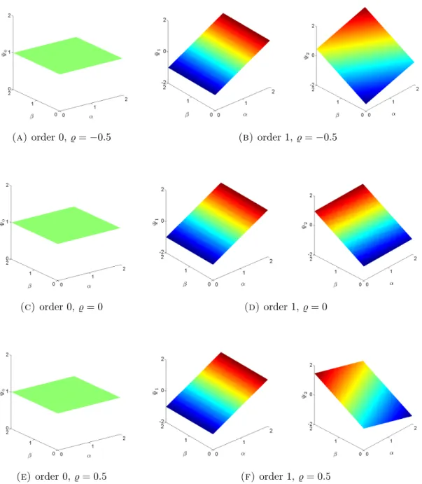
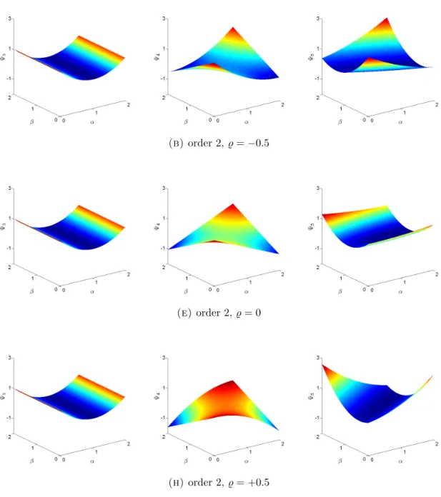
Figures 1-2 show all polynomials of order 0, 1 and 2 for correlation coefficients ̺ = {0,±0.5}. The plots show clearly the non-uniqueness of the orthogonal basis, viz., the influence of the ordering of the monic polynomials (7): the first polynomials of a new order, Φ{0,1,3}, are independent of the correlation coefficient and only determined
by the first monic polynomial e{0,1,3} of that order, the next ones of the same order,
Φ{2,4,5}, are different and dependent on the correlation. In Figure 3 we show the
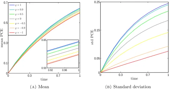
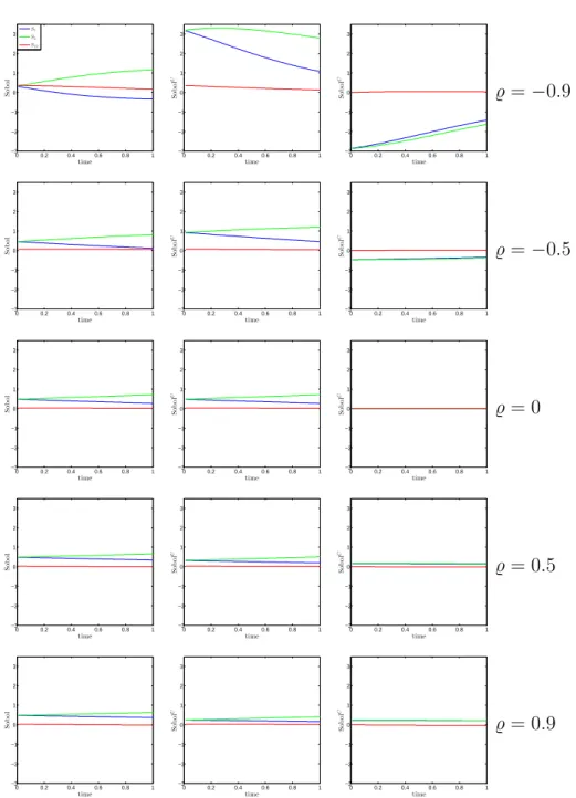
stochastic mean and standard deviation of the solution of Eq. (27) for the seven values of the correlation coefficient using a PCE expansion of 45 terms, which corresponds to a polynomial order of 8 and the polynomial basis calculated with the proposed method. The results are plot accurate, in the cases of no or full correlation with the ones obtained with the Hermite polynomial basis and same order, and with Monte Carlo simulations for the correlated distributions. The importance of propagating the true input distribution is especially seen in the standard deviation, where neither uncorrelated nor fully correlated give a reasonable approximation for a distribution with correlation ±0.5. This is also reflected in the Sobol’ indices. Figure 4 shows for all correlation coefficients the evolution of the Sobol’ indices (18) over time and the decomposition into the uncorrelated (19) and the correlated (20) part. These plots and Table 1 show how nicely the contributions of the variables itself and of the correlated variables follow the strength and sign of the correlation coefficient̺.
(a) order 0,̺=−0.5 (b)order 1,̺=−0.5
(c)order 0,̺= 0 (d) order 1,̺= 0
(e) order 0,̺= 0.5 (f) order 1,̺= 0.5
Figure 1. Polynomial basis. Order 0 and 1, for̺={0,±0.5}
diagonal, full correlation results in a zero variance, and no correlation gives a lower variance than correlation.
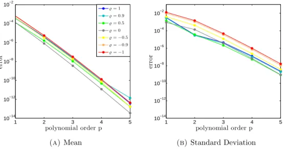
To answer the question whether the method has the same favourable convergence behavior as the original expansion for independent normal random variables (cf. [4]), we have performed an error convergence study using the following error measures
(b)order 2,̺=−0.5
(e) order 2,̺= 0
(h)order 2,̺= +0.5
Figure 2. Polynomial basis. Order 2, for ̺={0,±0.5}
wheretf = 1 is the final time point,µp andσp correspond to the mean and the standard
deviation obtained with PC expansion of orderp, andµexactandσexactare the reference
solutions, in this case obtained with p= 8.
0 0.3 0.7 1 0
0.1 0.3 0.5 0.7
time
m
e
a
n
P
C
E
̺= 1
̺= 0.9 ̺= 0.5
̺= 0
̺=−0.5
̺=−0.9
̺=−1
0.92 0.96 1 0.55
0.65
(a) Mean
0 0.3 0.7 1
0 0.05 0.15 0.25
time
st
d
P
C
E
(b) Standard deviation
Figure 3. Effect of correlation on mean and standard deviation of de-cay equation (27)
of the original PCE method for independently normally distributed input variables is conserved.
3.2. Enzymatic reaction. Consider the canonical enzymatic reaction
E + S ⇄k1 k2
C
C k3
→ E + P
where the concentrations of the substrate S, the enzyme E, the complex C, and the product P are the state variables and k1, k2, and k3 are the kinetic rate constants.
0 0.2 0.4 0.6 0.8 1 −3 −2 −1 0 1 2 3 time S o b o l S1 S2 S12
0 0.2 0.4 0.6 0.8 1 −3 −2 −1 0 1 2 3 time S o b o l U
0 0.2 0.4 0.6 0.8 1 −3 −2 −1 0 1 2 3 time S o b o l C
̺=−0.9
0 0.2 0.4 0.6 0.8 1 −3 −2 −1 0 1 2 3 time S o b o l
0 0.2 0.4 0.6 0.8 1 −3 −2 −1 0 1 2 3 time S o b o l U
0 0.2 0.4 0.6 0.8 1 −3 −2 −1 0 1 2 3 time S o b o l C
̺=−0.5
0 0.2 0.4 0.6 0.8 1 −3 −2 −1 0 1 2 3 time S o b o l
0 0.2 0.4 0.6 0.8 1 −3 −2 −1 0 1 2 3 time S o b o l U
0 0.2 0.4 0.6 0.8 1 −3 −2 −1 0 1 2 3 time S o b o l C
̺= 0
0 0.2 0.4 0.6 0.8 1 −3 −2 −1 0 1 2 3 time S o b o l
0 0.2 0.4 0.6 0.8 1 −3 −2 −1 0 1 2 3 time S o b o l U
0 0.2 0.4 0.6 0.8 1 −3 −2 −1 0 1 2 3 time S o b o l C
̺= 0.5
0 0.2 0.4 0.6 0.8 1 −3 −2 −1 0 1 2 3 time S o b o l
0 0.2 0.4 0.6 0.8 1 −3 −2 −1 0 1 2 3 time S o b o l U
0 0.2 0.4 0.6 0.8 1 −3 −2 −1 0 1 2 3 time S o b o l C
̺= 0.9
Figure 4. Dynamic plots of the Sobol’ indices of decay equation (27). Left: Sobol’ index, middle: contribution from the respective variables, right: contribution due to correlation with other variables.
given by the following system of ODEs:
dS¸(t)
dt = −k1E¸ (t)S¸(t) +k2C¸ (t) dC¸ (t)
dt = k1E¸ (t)S¸(t)−k2C¸ (t)−k3C¸ (t) dE¸ (t)
dt = −k1E¸ (t)S¸(t) +k2C¸ (t) +k3C¸ (t)
(31)
dP¸ (t)
̺ Si Siu Sic
S1 -0.337996430555719 1.079010380744548 -1.417006811300311
-0.9 S2 1.169072254592321 2.794020096839133 -1.624947842246789
S12 0.168924175966794 0.134133434465047 0.034790741501840
Sum 1.000000000003396 4.007163912048728 -3.007163912045260
S1 0.125070219450471 0.462450913298287 -0.337380693847799
-0.5 S2 0.819760985060438 1.197491238203163 -0.377730253142723
S12 0.055168795489075 0.037711983172792 0.017456812316329
Sum 0.999999999999984 1.697654134674242 -0.697654134674193
S1 0.273826682991019 0.273826682991019 0.000000000000004
0 S2 0.709059149322051 0.709059149322055 -0.000000000000000
S12 0.017114167686936 0.017114167686939 0.000000000000015
Sum 1.000000000000006 1.000000000000013 0.000000000000019
S1 0.340423008768462 0.196827595099748 0.143595413668727
0.5 S2 0.660699595355148 0.509674242072905 0.151025353282240
S12 -0.001122604123609 0.016050907606319 -0.017173511729914
Sum 1.000000000000001 0.722552744778972 0.311794278680881
S1 0.374323408284474 0.161822550653440 0.212500857631028
0.9 S2 0.636757390356394 0.419027897208577 0.217729493147815
S12 -0.011080798640891 0.020103679953051 -0.031184478593928
Sum 0.999999999999977 0.600954127815068 0.399045872184915
Table 1. Sobol’ indices and the contributions from variables itself and from correlated variables in the final timepoint tf = 1. The
respec-tive contributions follow nicely the strength and sign of the correlation coefficient.
Data for C¸ are available at regular intervals during the time interval [0,20] and the initial concentrations are known S¸(0) = 1, C¸ (0) = 0, E¸ (0) = 1, and P¸ (0) = 0. The parametersk1, k2, andk3 have been obtained by linear regression using the noisy data
for C¸ . The optimal value of the parameters in [2] was k = (0.683,0.312,0.212), with (independent) confidence intervals ∆ = [0.033,0.028,0.005]. To study the propaga-tion of the uncertainty through the model, the parameters are assumed to be random and their pdf is built based on the results in [2]. Thus, we assumed that the param-eters follow a uniform distribution with mean the optimal value of the paramparam-eters
1 2 3 4 5 10−14
10−12 10−10 10−8 10−6 10−4 10−2
polynomial order p
er
ro
r
̺= 1
̺= 0.9
̺= 0.5
̺= 0
̺=−0.5
̺=−0.9
̺=−1
(a) Mean
1 2 3 4 5
10−14 10−12 10−10 10−8 10−6 10−4 10−2
polynomial order p
er
ro
r
(b)Standard Deviation
Figure 5. Convergence of the error in mean and standard deviation for the decay equation (27)
avoid entering the non-physical negative parameter space), andC the correlation ma-trix also obtained from the Fisher information mama-trix; as in the previous example, the fully correlated case, Cf, and the uncorrelated case,Cu, are also studied
C=
1 0.9 −0.37 0.9 1 −0.45 −0.37 −0.45 1
Cf =
1 1 −1 1 1 −1 −1 −1 1
Cu =
1 0 0 0 1 0 0 0 1
As the analytic expression for the pdf of the joint distribution of two or more correlated uniform variables is unknown, we cannot use the moment-generating function to calcu-late all the required moments. Therefore, Monte Carlo integration will be used in this example. To generate sampling points from a correlated multidimensional uniform distribution we used the standard approach of computing them from the correlated normal distribution (see, e.g., [6]). Again, the problem collapses to one-dimensional in the fully correlated case, correlation matrix Cf. The only parameter in this case
follows the standard uniform distribution U(0,1).
0 5 10 15 20 0 0.2 0.4 0.6 0.8 1 time m ea n P C E Cu C Cf Sol det (a) S¸
0 5 10 15 20
0 0.2 0.4 0.6 0.8 1 time m ea n P C E
(b) E¸
0 5 10 15 20
0 0.2 0.4 0.6 0.8 1 time m ea n P C E
(c)P¸
Figure 6. Mean of the stochastic state variables of Eq. (32).
0 5 10 15 20
0 0.04 0.08 0.12 time st d P C E Cu C Cf (a) S¸
0 5 10 15 20
0 0.04 0.08 0.12 time st d P C E
(b)C¸ and E¸
0 5 10 15 20
0 0.04 0.08 0.12 time st d P C E
(c)P¸
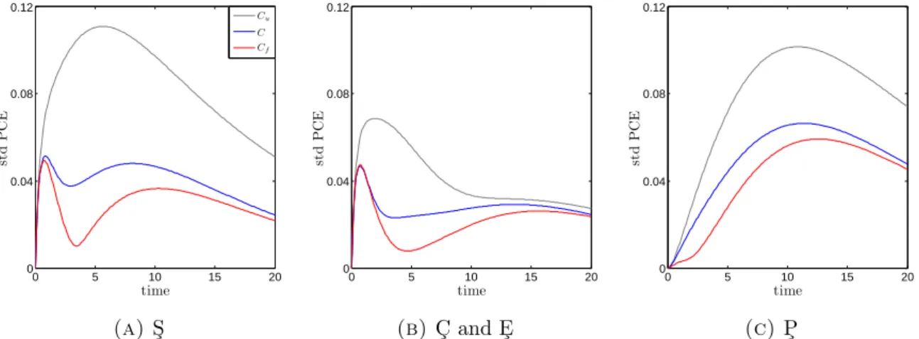
Figure 7. Standard deviation of the stochastic state variables of Eq. (32) for the uncorrelated case (grey), the fully correlated case (red), and the correlation matrix resulting from the experimental errors (blue).
0 5 10 15 20 0
0.2 0.4 0.6 0.8 1
time
S
o
b
o
l
(a) S¸
0 5 10 15 20
0 0.2 0.4 0.6 0.8 1
time
S
o
b
o
l
(b)C¸ and E¸
0 5 10 15 20
0 0.2 0.4 0.6 0.8 1
time
S
o
b
o
l
(c)P¸
Figure 8. Dynamic plots of the Sobol’ indices of the enzymatic reaction (32) for the uncorrelated case.
from the variable itself, resulting in a small Sobol’ value, but fixing such a variable would have a large impact on the outcome.
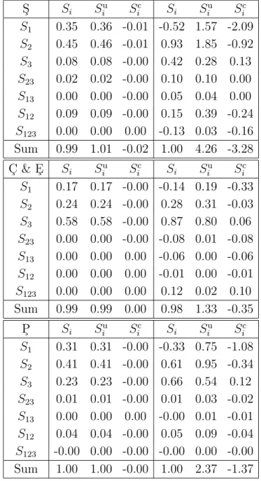
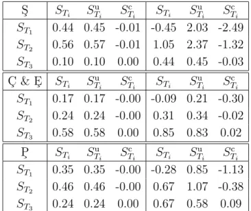
Ranking variables is often done based on the Sobol’ indices. Depending on the time-frame of interest, one can use as measure, e.g., the integral over time of the Sobol’ indices, or the Sobol’ indices in a specific point. As an example of the latter we study at the final time-point, tf = 20, which part of the variance of the concentrations
is due to the variance of respective input variables. Tables 2 and 3 give the Sobol’ indices and the total Sobol’ indices, respectively, for the random variables k1, k2, and
k3. Note that the sum of the Sobol’ indices equals one and for the uncorrelated case
the Sc values should be zero, so the deviation of these values gives the error in the
approximation, in this case mostly due to the approximation of the high-order moments needed for the Sobol’ indices. From Table 3 one can deduce that, in the uncorrelated case, decomposing the variance of the concentration of the substrate S would lead to the conclusion that the random variable k3 can be fixed to the nominal deterministic
value, since its influence on the variance of S is negligible. In the correlated case, however, this is no longer true. One can also see that especially for k1 and k2 the
interpretation of the Sobol’ indices is not trivial, e.g., for C the influence of k1 is very
small but this is due to cancellation of the Su and Sc contribution. As stated before,
S¸
C¸ and E¸
P¸
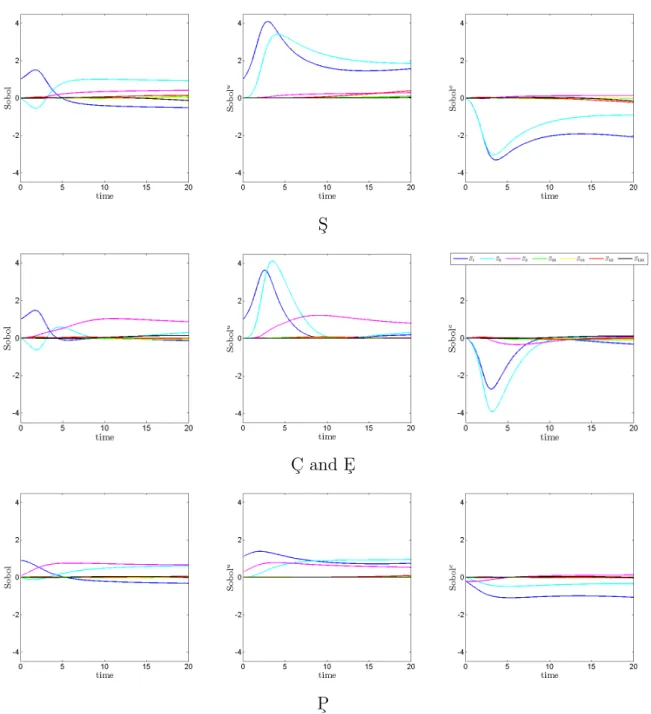
Figure 9. Dynamic plots of the Sobol’ indices of enzymatic reaction (32), for the correlation matrix resulting from the experimental errors. Left: Sobol’ indexS, middle: contribution from the respective variables,
Su, right: contribution due to correlation with other variables, Sc.
4. Discussion and concluding remarks
S¸ Si Siu S c
i Si Siu S
c i
S1 0.35 0.36 -0.01 -0.52 1.57 -2.09
S2 0.45 0.46 -0.01 0.93 1.85 -0.92
S3 0.08 0.08 -0.00 0.42 0.28 0.13
S23 0.02 0.02 -0.00 0.10 0.10 0.00
S13 0.00 0.00 -0.00 0.05 0.04 0.00
S12 0.09 0.09 -0.00 0.15 0.39 -0.24
S123 0.00 0.00 0.00 -0.13 0.03 -0.16
Sum 0.99 1.01 -0.02 1.00 4.26 -3.28 C¸ & E¸ Si Siu S
c
i Si Siu S
c i
S1 0.17 0.17 -0.00 -0.14 0.19 -0.33
S2 0.24 0.24 -0.00 0.28 0.31 -0.03
S3 0.58 0.58 -0.00 0.87 0.80 0.06
S23 0.00 0.00 -0.00 -0.08 0.01 -0.08
S13 0.00 0.00 0.00 -0.06 0.00 -0.06
S12 0.00 0.00 0.00 -0.01 0.00 -0.01
S123 0.00 0.00 0.00 0.12 0.02 0.10
Sum 0.99 0.99 0.00 0.98 1.33 -0.35 P¸ Si Siu S
c
i Si Siu S
c i
S1 0.31 0.31 -0.00 -0.33 0.75 -1.08
S2 0.41 0.41 -0.00 0.61 0.95 -0.34
S3 0.23 0.23 -0.00 0.66 0.54 0.12
S23 0.01 0.01 -0.00 0.01 0.03 -0.02
S13 0.00 0.00 0.00 -0.00 0.01 -0.01
S12 0.04 0.04 -0.00 0.05 0.09 -0.04
S123 -0.00 0.00 -0.00 -0.00 0.00 -0.00
Sum 1.00 1.00 -0.00 1.00 2.37 -1.37
Table 2. Sobol’ indices in the final time point tf = 20. The left part
of the table corresponds to the uncorrelated case, correlation matrix
Cu; the right part to the correlation matrix C obtained from the FIM.
The columnsSu
i show the contribution from the variables itself and the
columnsSc
i the contribution from correlated variables; with exact
com-putations theSc
i-column in the left part of the table should be zero.
S¸ STi S
u
Ti S
c
Ti STi S
u
Ti S
c Ti ST1 0.44 0.45 -0.01 -0.45 2.03 -2.49
ST2 0.56 0.57 -0.01 1.05 2.37 -1.32
ST3 0.10 0.10 0.00 0.44 0.45 -0.03
C¸ & E¸ STi S
u
Ti S
c
Ti STi S
u
Ti S
c Ti ST1 0.17 0.17 -0.00 -0.09 0.21 -0.30
ST2 0.24 0.24 -0.00 0.31 0.34 -0.02
ST3 0.58 0.58 0.00 0.85 0.83 0.02
P¸ STi S
u
Ti S
c
Ti STi S
u
Ti S
c Ti ST1 0.35 0.35 -0.00 -0.28 0.85 -1.13
ST2 0.46 0.46 -0.00 0.67 1.07 -0.38
ST3 0.24 0.24 0.00 0.67 0.58 0.09
Table 3. Total Sobol’ indices in the final time point tf = 20. The left
part of the table corresponds to the uncorrelated case, correlation matrix
Cu; the right part to the correlation matrix C obtained from the FIM.
for the current PCE implementations. This method makes it possible to compute for a set of random input variables with any multivariate distribution, including an experimentally determined one, the stochastic distribution of a Quantity of Interest. An application we studied is the true propagation of experimental errors through the parameter-fitting process onto the state variables, so that a QoI based on these state variables is described as a distribution and, e.g., optimal experimental design can be applied to reduce the variance in such a QoI. In this paper we used either exact integra-tion or Monte Carlo to compute the moments and the projecintegra-tion onto the polynomial basis, but for the latter Gauss quadrature is under development.
There are a few remarks to make with respect to the method
• As for other PCE methods, the polynomial base is only dependent on the multivariate distribution of the random input variables. Once computed, all problems with random input variables described by this pdf can be solved using the same base.
If the correlation coefficient̺ equals 0.9 the latter order of magnitude is even much higher: 1021 for moments of order 75.
• The orthogonal polynomial basis is not unique, it is dependent on the choice and ordering of the original set of linearly independent polynomials. It is an open question at the moment whether there is an optimal choice for this original set of polynomials, e.g., to reduce the magnitude of the moments required or to simplify computations.
• Whereas in the uncorrelated case interpretation of Sobol’ indices and ranking of the influence of the variation of the random input variables on the variance in the QoI is more or less straighforward, this is no longer true for correlated random variables.
Acknowledgements
References
[1] H.L. Anderson, Metropolis, Monte Carlo and the MANIAC, Los Alamos Science, 14, 96-108, 1986.
[2] M. Ashyraliyev, Y. Fomekong-Nanfack, J.A. Kaandorp, J.G. Blom, Systems biology: parameter estimation for biochemical models, The FEBS Journal, 276(4), 886-902, 2009.
[3] A.J. Brown, Enzyme action, J. Chem. Soc. 81, 373-386, 1902.
[4] R. Cameron, W. Martin, The orthogonal development of nonlinear functionals in series of Fourier-Hermite functionals, Annals of Mathematics, 48, 385-392, 1947.
[5] J.L. Castro, M. Navarro, J.M. S´anchez, J.M. Zurita, Loss and gain functions for CBR retrieval, Information Sciences, 179(11), 1738-1750, 2009.
[6] C.T.S. Dias, A. Samaranayaka, B. Manly, On the use of correlated beta random variables with animal population modelling, Ecological Modelling, 215, 293-300, 2008.
[7] M.S. Eldred, C.G. Webster, P.G. Constantine, Evaluation of non-intrusive approaches for Wiener-Askey generalized polynomial chaos, AIAA 2008-1892, 2008.
[8] B. Fox, Strategies for Quasi-Monte Carlo, Kluwer academic Pub., 1999.
[9] V. Golosnoy, Y. Okhrin, General uncertainty in portfolio selection: A case-based decision ap-proach, Journal of Economic Behavior & Organization, 67, (3-4), 718-734, 2008.
[10] G.H. Golub, C.F. van Loan, Matrix computations (third edition), The John Hopkins University Press, Baltimore and London, 1996.
[11] T.Y. Hou, W. Luo, B. Rozovskii, H.-M. Zhou, Wiener chaos expansions and numerical solutions of randomly forced equations of fluid mechanics, Journal of Computational Physics, 216(2), 687-706, 2006.
[12] F.S. Hover, M.S. Triantafyllou, Application of polynomial chaos in stability and control, Auto-matica, 42(5), 789-795, 2006.
[13] M. Kleiber, T.D. Hien, The stochastic finite element method: basic perturbation technique and computer implementation, Wiley, 1992.
[14] R.H. Kraichnan, Direct-interaction approximation for a system of several interacting simple shear waves, The Physics of Fluids, 6(11), 1603-1609, 1963.
[15] G. Li, H. Rabitz, P.E. Yelvington, O.O. Oluwole, F. Bacon, C.E. Kolb, J. Schoendorf, Global sen-sitivity analysis for systems with independent and/or correlated inputs, The Journal of Physical Chemistry A, 114(19), 6022-6032, 2010.
[16] H. Li, D. Zhang, Probabilistic collocation method for flow in porous media: comparisons with other stochastic methods, Water Resources Research, 43, 44-48, 2009.
[17] W. Loh, On Latin hypercube sampling, Annals of Statistics, 24, 2058-2080, 1996.
[18] J.L. Lumley, The structure of inhomogeneous turbulent flows, In Atmospheric Turbulence and Wave Propagation, ed. A.M. Yaglom, V.I. Tatarski, 166-178, 1967.
[19] N. Madras, Lectures on Monte Carlo methods, American Mathematical Society, Providence, RI, 2002.
[20] MATLAB and Symbolic Math Toolbox Release 2012b, The MathWorks, Inc., Natick, Mas-sachusetts, United States.
[22] A. Nataf, D´etermination des distributions de probabilit´es dont les marges sont donn´ees, Comptes Rendus de l’Acad´emie des Sciences, 225, 42-43, 1962.
[23] S. Oladyshkin, W. Nowak, Data-driven uncertainty quantification using the arbitrary polynomial chaos expansion, Reliability Engineering & System Safety, 106, 179-190, 2012.
[24] S.A. Orszag, L.R. Bissonnette, Dynamical properties of truncated Wiener-Hermite expansions, The Physics of Fluids, 10(12), 2603-2613, 1967.
[25] A.B. Owen, Variance components and generalized Sobol’ indices, SIAM/ASA J. Uncertainty Quantification 1(1), 19-41, 2013.
[26] M. Rajaschekhar, B. Ellingwood, A new look at the response surface approach for reliability analysis, Structural Safety, 123, 205-220, 1993.
[27] M. Rosenblatt, Remarks on a multivariate transformation, The Annals of Mathematical Statis-tics, 23(3), 470-472, 1952.
[28] E. Schmidt, Zur Theorie der linearen und nichtlinearen Integralgleichungen. I. Teil: Entwicklung willk¨urlicher Funktionen nach Systemen vorgeschriebener, Math. Ann., 63, 433-476, 1907. [29] P. Schola, O.P. Le Maitre, Polynomial chaos expansion for subsurface flows with uncertain soil
parameters, Advances in Water Resources, 62, Part A, 139-154, 2013.
[30] C. Soize, R. Ghanem, Physical systems with random uncertainties: chaos representations with arbitrary probability measure, SIAM Journal on Scientific Computing, 26(2), 395-410, 2004. [31] I.M. Sobol’, Sensitivity estimates for nonlinear mathematical models, Math. Modeling & Comput.
Exp., 1, 407-414, 1993.
[32] B. Sudret, Global sensitivity analysis using polynomial chaos expansions, Reliability Engineering & System Safety, 93(7), 964-979, 2008.
[33] H. Hotelling, M.R. Pabst, Rank correlation and test of significance involving no assumption of normality, Annals of Mathematical Statistic, 7, 29-43, 1936.
[34] M. Villegas, F. Augustin, A. Gilg, A. Hmaidi, U. Wever, Application of the polynomial Cchaos expansion to the simulation of chemical reactors with uncertainties, Mathematics and Computers in Simulation, 82(5), 805-817, 2012.
[35] X. Wan, G.E. Karniadakis, Beyond Wiener-Askey expansions: handling arbitrary PDFs, Journal of Scientific Computing, 27(1-3), 455-464, 2006.
[36] N. Wiener, The homogeneous chaos, American Journal of Mathematics, 60(4), 897-936, 1938. [37] J.A.S. Witteveen, H. Bijl, Efficient quantification of the effect of uncertainties in
advection-diffusion problems using polynomial chaos, Numerical Heat Transfer B: Fundamentals, 53, 437-465, 2008.
[38] J.A.S. Witteveen, S. Sarkar, H. Bijl, Modeling physical uncertainties in dynamic stall induced fluid-structure interaction of turbine blades using arbitrary polynomial chaos, Computers and Structures, 85, 866-878, 2007.
[39] J.A.S. Witteveen, H. Bijl, Modeling arbitrary uncertainties using Gram-Schmidt polynomial chaos, AIAA-2006-896, 44th AIAA Aerospace Sciences Meeting and Exhibit, Reno, Nevada, 2006.
[40] D. Xiu, Efficient collocational approach for parametric uncertainty analysis, Communications in Computational Physics, 2(2), 293-309, 2007.