www.hydrol-earth-syst-sci.net/13/503/2009/ © Author(s) 2009. This work is distributed under the Creative Commons Attribution 3.0 License.
Earth System
Sciences
Sensitivity analysis and parameter estimation for distributed
hydrological modeling: potential of variational methods
W. Castaings1,2,4, D. Dartus1, F.-X. Le Dimet2, and G.-M. Saulnier3
1IMFT UMR 5502 (CNRS, INP, UPS), Universit´e de Toulouse, 31400 Toulouse Cedex, France 2LJK UMR 5224 (CNRS, INPG, UJF, INRIA), Grenoble Universit´es, 38041 Grenoble Cedex 9, France 3EDYTEM, UMR 5204, Universit´e de Savoie, 73376 Le Bourget du Lac Cedex, France
4European Commission, Directorate-General Joint Research Centre, Institute for the Protection and Security of the Citizen, Econometrics and Applied Statistics Unit, T.P. 361, 21020 Ispra (VA), Italy
Received: 17 January 2007 – Published in Hydrol. Earth Syst. Sci. Discuss.: 22 February 2007 Revised: 31 March 2009 – Accepted: 31 March 2009 – Published: 24 April 2009
Abstract. Variational methods are widely used for the
anal-ysis and control of computationally intensive spatially dis-tributed systems. In particular, the adjoint state method en-ables a very efficient calculation of the derivatives of an ob-jective function (response function to be analysed or cost function to be optimised) with respect to model inputs.
In this contribution, it is shown that the potential of vari-ational methods for distributed catchment scale hydrology should be considered. A distributed flash flood model, cou-pling kinematic wave overland flow and Green Ampt infil-tration, is applied to a small catchment of the Thor´e basin and used as a relatively simple (synthetic observations) but didactic application case.
It is shown that forward and adjoint sensitivity analysis provide a local but extensive insight on the relation between the assigned model parameters and the simulated hydrologi-cal response. Spatially distributed parameter sensitivities can be obtained for a very modest calculation effort (∼6 times the computing time of a single model run) and the singular value decomposition (SVD) of the Jacobian matrix provides an in-teresting perspective for the analysis of the rainfall-runoff re-lation.
For the estimation of model parameters, adjoint-based derivatives were found exceedingly efficient in driving a bound-constrained quasi-Newton algorithm. The reference parameter set is retrieved independently from the optimiza-tion initial condioptimiza-tion when the very common dimension re-duction strategy (i.e. scalar multipliers) is adopted.
Correspondence to:W. Castaings
Furthermore, the sensitivity analysis results suggest that most of the variability in this high-dimensional parameter space can be captured with a few orthogonal directions. A parametrization based on the SVD leading singular vec-tors was found very promising but should be combined with another regularization strategy in order to prevent overfitting.
1 Introduction
The distributed modelling of catchment hydrology is now recognised as a valuable approach in order to understand, re-produce and predict the behavior of hydrological systems. However, distributed hydrological models remain a simpli-fied and imperfect representation of the physical processes using uncertain observation data for the estimation of the model inputs to be prescribed (parameters, initial condition and rainfall forcing). Analyzing and reducing uncertainty is therefore essential but issues such as sensitivity and un-certainty analysis, parameter estimation and state-updating are challenging given the dimensionality of the system. Al-though the approach adopted in this paper is not restricted to a specific type of model input, the focus will be on model pa-rameters to be assigned on the basis of indirect observations (i.e. model calibration).
Experiences in the calibration of such models revealed that the corresponding response surface often contains sev-eral regions of attraction, discontinuous derivatives and other geometrical properties compromising the use of local methods, especially those using derivative information (Ib-bit and O’Donnell, 1971; Johnston and Pilgrim, 1976; Duan et al., 1992).
Therefore, many recent applications and methodologi-cal developments for model methodologi-calibration involve a stochas-tic exploration of the parameter space using computation-ally intensive Monte Carlo methods and/or evolutionary al-gorithms. These techniques enable the global optimization of single or multiple objectives and very often characterise the uncertainty affecting model parameters (Beven and Bin-ley, 1992; Duan et al., 1992; Kuczera and Parent, 1998; Yapo et al., 1997; Vrugt et al., 2003a,b).
Differential sensitivity analysis (McCuen, 1973a,b), which was very often the only approach computationally afford-able, is now gradually replaced by assessments carried out in the statistical framework. The Regional Sensitivity Analy-sis (RSA) of Hornberger and Spear (1981) inspired numer-ous applications and developments for the analysis of hy-drological systems including the contribution of Beven and Binley (1992). The combination with recursive estimation techniques (Vrugt et al., 2002; Wagener et al., 2003) or the extension to multiple objectives (Bastidas et al., 1999) can provide an interesting insight into the behaviour of hy-drological models. The use of variance decomposition ap-proaches which are based on unambiguous importance mea-sures (Cukier et al., 1978; Sobol’, 1993; Homma and Saltelli, 1996) is now emerging in the hydrological community (Tang et al., 2007a,b; Yatheendradas et al., 2008; Van Werkhoven et al., 2008a). Using these global sensitivity analysis tech-niques, it is possible to assess how uncertainty in the model outputs can be apportioned to different sources of uncertainty in the model inputs (Saltelli et al., 2000).
When parameter estimation and sensitivity analysis are carried out in the statistical framework, it is necessary to sample the space of uncertain inputs. However, in distributed hydrological models, parameters are discretized according to the spatial discretization of the model state variables. Ap-proaches developed for parsimonious hydrological models are frequently transferred to distributed hydrological mod-els by means of an empirical dimension reduction of the pa-rameter space. For papa-rameter estimation, scalar multipliers are used in order to adjust spatially distributed parameters featuring a variability which is fixed using prior information (Refsgaard, 1997; Madsen, 2003). The same strategy can be adopted for probabilistic sensitivity analysis (Yatheendradas et al., 2008). In some cases, spatially distributed impor-tance measures are estimated for a very coarse grid resolu-tion or few zones of constant value (Hall et al., 2005; Tang et al., 2007a; Van Werkhoven et al., 2008b). Sampling based approaches to sensitivity analysis and parameter estimation enable an exploration of the parameter space (essential for
non-linear systems) but can be limited in handling distributed parameter systems (i.e. curse of dimensionality).
In the deterministic framework, both sensitivity analy-sis and parameter estimation can be addressed using varia-tional methods. The adjoint state method enables an effi-cient calculation of the derivatives of an objective function with respect to all model inputs. This technique is particu-larly suited when the dimension of the response function to be analysed or cost function to be optimized is small when compared to the number of inputs to be prescribed (Lions, 1968; Cacuci, 1981a; Le Dimet and Talagrand, 1986). It has contributed to numerous applications related to the anal-ysis and forecasting of meteorological and oceanographic systems (Le Dimet and Talagrand, 1986; Hall and Cacuci, 1983; Navon, 1998; Ghil and Malanotte-Rizzoli, 1991; Ben-nett, 1992). Early applications of the adjoint state method to hydrological systems have been carried out in groundwa-ter hydrology (Chavent, 1974; Carrera and Neuman, 1986; Sun and Yeh, 1990). The resolution of inverse problems (pa-rameter, state and boundary condition estimation), local sen-sitivity analysis, where also addressed in this framework in land surface hydrology (Mahfouf, 1991; Callies et al., 1998; Calvet et al., 1998; Bouyssel et al., 1999; Margulis and En-tekhabi, 2001; Reichle et al., 2001), vadose zone hydrology (Ngnepieba et al., 2002), river and floodplain hydraulics (Pi-asecki and Katopodes, 1997; Belanger and Vincent, 2005; Honnorat et al., 2006) and catchment hydrology (White et al., 2003; Seo et al., 2003a).
The previously mentioned applications involve non-linear models and the underlying inverse problems (i.e. parameter estimation and state updating) are ill-posed. For example, equifinality is inherent in the estimation of a distributed hy-draulic conductivity in groundwater hydrology or in the esti-mation of an initial state for the atmosphere in meteorology. The estimation of model inputs require an appropriate com-bination of prior information (e.g. derived from land cover and soil type) and observations of the model diagnostic vari-ables (e.g. streamflow observations). The variational frame-work is suitable for the combination of the different sources of information (including statistical information) trough the resolution of a regularized inverse problem.
valid for a specific point of the parameter space) but provide tremendous information which would require a prohibitive computational cost if it is was to be obtained using sampling based approaches.
In rainfall-runoff modelling, deterministic sensitivity anal-ysis and gradient-based parameter estimation have been used in the past and the contributions of McCuen (1973a,b) and Gupta and Sorooshian (1985) are directly in line with the current research endeavor. The explicit but piecewise differ-entiation (i.e. analytic derivatives rather than classical finite difference approximation) carried out by McCuen (1973a) and Gupta and Sorooshian (1985) corresponds to the strategy adopted for the forward mode of algorithmic differentiation (Rall, 1981). By making the computational cost indepen-dent from the dimension of the input space the adjoint state method (implemented with the reverse mode of algorithmic differentiation) represents a significant improvement for the analysis and control of spatially distributed hydrological sys-tems. The contributions of White et al. (2003) and Seo et al. (2003a,b) address the use of this approach for parameter es-timation and state updating.
The objective of this paper is to demonstrate the potential of variational methods, briefly presented in Sect. 2, for the analysis of distributed rainfall-runoff models. A very simple application case is adopted for this prospective study. Other investigations involving more complex configurations and other model structures were carried out and will be reported in due course. A distributed flash flood model described in Sect. 3 was applied to a small catchment of the Thor´e basin. The authors seek to illustrate what can be learned or corrob-orated using forward and adjoint sensitivity analysis for un-derstanding the mapping between the model parameters and the simulated hydrological response. Using synthetic obser-vations, the ability of efficient adjoint-based optimization to estimate reliable values for the model parameters is investi-gated. The results of sensitivity analysis and parameter es-timation experiments are provided in Sects. 4 and 5 and the paper is concluded by a discussion of the main outcomes.
2 Variational methods for sensitivity analysis and
parameter estimation
Variational methods provide a deterministic framework for the analysis and control of physical systems. The mathemat-ical formalism, based on functional analysis and differential calculus, was largely expanded by related scientific disci-plines such as optimal control and optimization. Adopting the vocabulary of optimal control theory, model parameters, initial and boundary conditions are referred as control vari-ables living in a so-called control space.
This differential approach enables the exact calculation of the derivatives of a function of the model prognostic vari-ables with respect to all control varivari-ables. Using the ad-joint state method, the computational cost can be
indepen-dent from the dimension of the control space. It is precisely this feature which makes the approach very attractive for the analysis and control of spatially distributed systems.
Although any control variable can be analysed, the focus of this paper is parametric uncertainty. The use of deriva-tives for local sensitivity analysis and parameter estimation is addressed in Sects. 4 and 5. In this section, the calculation strategy is briefly described using a simplified mathematical formalism and the practical implementation of the approach is discussed.
For a didactic presentation of the approach, let us consider that the behavior of the system between timest0 andtf is
described by a generic model of the form:
∂x
∂t =M(x,α)
x(t0)=0
(1)
wherexis the state variable of dimensionNs,Ma nonlinear
operator (after space discretization) andαa vector of param-eters of dimensionNp. When the model parameters are fixed
toα=α¯,x¯the corresponding nominal value for the state vari-ablexis obtained by solving the system given by Eq. (1).
In order to analyse or control the behaviour of the system, let us define a generic objective functional:
J (x,α)=
Z tf
t0
φ (t;x,α)dt (2)
whereφ is a nonlinear function of the state variables and model parameters. The objective functionJ can represent a specific aspect of the system behaviour (i.e. response func-tion) or quantify the misfit between the model diagnostic variables and the available observations (i.e. cost function).
The gradient of the functionalJ (real valued scalar func-tion) with respect toαat the pointα¯ is given by
∇αJ (x¯,α¯)= ∂J ∂α1
, . . . , ∂J ∂αNp
!
¯
α
(3)
The components of this vector quantify the rate of change of J along the vectors of the standard basis in the param-eter space. After the application of a normalization proce-dure (discussed in Sect. 4), importance measures can be esti-mated in order to compare the relative influence of the vari-ous model parameters on the response of interest. WhenJis a cost function to be optimized,∇αJcan drive very efficient
gradient-based optimization algorithms (e.g. quasi-newton) for the estimation of model parameters.
2.1 Problems underlying the approximation
of derivatives
for the evaluation of the gradient components consists in re-peated model evaluations. For example, the first order finite difference approximation for thei-th component is given by
∂J ∂αi
¯
α
≈J (α¯1, . . . ,α¯i+ε, . . . ,α¯Np)−J (α¯)
ε (4)
where ε refers to a perturbation applied to the nominal value ofαi. Using this approach, the model can be
con-sidered as a black box and the practical implementation is straightforward. However, the precision and efficiency of this technique are very limited. The accuracy of the ap-proximation crucially depends on choice of the step sizeε. In practice, there is a very difficult compromise to be found. Large values of ε lead to truncation error, small values may give rise to cancellation/round-off error. More-over, for the approximation of all gradient components (i.e. ∂J /∂αi i=1, . . . , Np), perturbations should be applied
along all vectors of the canonical basis ofRNp. Using the first order finite difference approximation given by Eq. 4, Np+1 model evaluations are necessary. This number is of
course larger for higher order approximations. Therefore, the overall computational cost is at least linearly related to the dimension of the parameter space.
In order to avoid the use of a perturbation parameterε, derivatives can be calculated analytically. A very general and comprehensive mathematical formalism for differential sensitivity analysis was proposed by Cacuci (1981a,b). It is based on the concept of Gˆateaux derivative, a generalisation of the concept of directional derivative in differential calcu-lus.
2.2 Forward sensitivity analysis
The derivative of the objective functionJ at the pointα¯ in the directionαˆ is given by:
ˆ
J (α¯,αˆ)=
Z tf
t0 ∂φ ∂x ¯ α ˆ x+ ∂φ ∂α ¯ α ˆ α dt (5)
wherexˆ refers to variations on the state variablexresulting from perturbations on the parametersαin the directionαˆ. It is important to note thatJ (ˆ α¯,αˆ)=
∇αJ,αˆ (h,i standing
for the scalar product). Given thatxis governed by Eq. (1), it is necessary to derive this system in order to estimatexˆ. Therefore,xˆis solution of the following system:
∂xˆ
∂t− ∂M ∂x ¯ α ˆ x= ∂M ∂α ¯ α ˆ α ˆ
x(t0)=0
(6)
where [∂M/∂x] represents the Jacobian of the model with respect to the state variables and [∂M/∂α] the Jacobian of the model with respect to the model parameters.
The system given by Eq. (6) is the so-called tangent lin-ear model (TLM). For a given perturbation αˆ, xˆ is ob-tained by the resolution of the TLM. The resulting varia-tion of the objective funcvaria-tion (e.g. J (ˆ α¯,αˆ)) can be calcu-lated from Eq. (5).
However, in order to obtain all gradient components, the operation should be repeated forαˆ corresponding to the dif-ferent vectors of the canonical basis ofRNp. This means that the resolution of the TLM has to be carried out for each direc-tionαˆ. Therefore, the precision problem (i.e. approximation error) is addressed but the overall computational cost is still dependent on the dimension of the parameter space. This difficulty can be overcome by using the adjoint state method.
2.3 Adjoint sensitivity analysis
The linearity ofJ (ˆα¯,αˆ)with respect toαˆ is produced using the introduction of an auxiliary variablep(of dimensionNs).
It can be shown (Cacuci, 1981a; Le Dimet and Talagrand, 1986) that ifpis governed by the following system
∂p ∂t + ∂M ∂x T ¯ α p= ∂φ ∂x ¯ α p(tf)=0
(7)
the gradient is given by
∇αJ (x¯,α¯)= Z tf
t0 ∂φ ∂α ¯ α − ∂M ∂α T ¯ α p ! dt (8)
where [ ]T stands for the transpose.
It is important to note thatxˆandαˆdo not appear in Eqs. (7) and (8). Therefore, oncepis known by integration (back-ward in time) of the system described by Eq. (7), all the com-ponents of the gradient∇αJ needed for sensitivity analysis
and parameter estimation can be calculated. In the math-ematical optimization framework, the objective is to maxi-mize/minimise the cost functionJ whilexis subject to the constraint given by Eq. 1 (i.e. x should verify the govern-ing equations). In this case, the adjoint variables correspond to the Lagrange multipliers of the constrained optimization problem. The principal difficulty resides in the derivation and transposition of complex operators.
2.4 Practical implementation
In principle, forward and adjoint sensitivity analysis can be performed on the continuous or discrete formulation of the model. Different implementation strategies can be adopted depending if the derivation and transposition operations are carried out on the continuous form of the direct model, on its discretized form or directly on the computer code. Algo-rithmic differentiation (AD) is usually preferred (see Sei and Symes, 1995 or Sirkes and Tziperman, 1997 for counterex-amples) for reliable and accurate derivatives. The reader is referred to Griewank (2000) for a comprehensive description of AD.
rule (e.g. product of local Jacobians) in the forward or re-verse direction. In order to use this discrete equivalent of forward and adjoint sensitivity analysis methods, the source code of the model should be available. The availability of au-tomatic differentiation engines (see http://www.autodiff.org/) provide a helpful and efficient support for the practical im-plementation of variational methods. It is important to em-phasise that using this implementation strategy, the potential on-off switches characterising the representation of physi-cal processes (i.e. thresholds in model formulation) are sim-ply reported in the TLM and ADM (Zou et al., 1993). The derivative provided by AD is therefore an element of the sub-gradient.
3 Flash flood model
A very simple and common model structure was adopted and applied to a small catchment using synthetic observations. An event-based distributed rainfall-runoff model is applied to a small area in the upper part of the Thor´e catchment (Tarn department, South West of France).
3.1 Model description
The underlying physics of MARINE flash flood model (Estupina-Borrell et al., 2006) is adapted to events for which infiltration excess dominates the generation of the flood. A simplified version of the model is used for this prospective study. Rainfall abstractions are evaluated using the Green Ampt infiltration model and the resulting surface runoff is transferred using the Kinematic wave approximation (KWA). The complex geometry of the catchment is described by a structured grid in which each cell receives water from its ups-lope neighbors and discharge to a single downsups-lope neighbor (steepest direction).
For a one dimensional flow of average velocityuand av-erage depthh, the continuity equation can be expressed as:
∂h ∂t +
∂uh
∂x =r−i (9)
whereris the rainfall intensity andithe infiltration rate. Us-ing the KWA approximation, which has shown the ability to represent channelized and sheet overland flow (Singh, 2001), the momentum conservation equation reduces to an equilib-rium between the bed slopeS0and the friction slopeSf. The
Manning equation (uniform flow on each grid cell) is used to relate the flow velocity and the flow depth:
u= R
2/3S1/2
f
n with R=
hw
2h+w (10)
whereR is the hydraulic radius,n the Manning roughness coefficient andwthe elemental flow width. In this simplified version of the model, the flow width is constant (rectangular section) and given the ratio between the width (grid resolu-tion) and the flow depth the hydraulic radius is approximated
by the water depth (i.e.R=h). The resulting equation gov-erning the overland flow is given by:
∂h ∂t +
S01/2 n
∂h5/3
∂x =r−i (11)
In the right hand side of Eq. (11), the infiltration ratei(t ) is estimated using the very common Green-Ampt infiltration model.
For an homogeneous soil column characterised by its ef-fective hydraulic conductivityK,ψ the soil suction at wet-ting front, the potential infiltration rate is given by
i(t )=K ψ 1θ
I (t ) +1
with 1θ=η(1−θ ) (12) whereθis the relative initial soil moisture (i.e.θ∈[0,1]),η the soil porosity andI (t )the cumulative infiltration at time t. After surface ponding, the cumulative infiltration at time t+1tcan be calculated by the following equation
It+1t −It−ψ 1θln
I
t+1t+ψ 1θ
It+ψ 1θ
=K1t (13)
which is solved by Newton’s method.
In order to carry out the sensitivity analysis and parameter estimation experiments presented in Sects. 4 and 5, it is nec-essary to implement the tangent linear and adjoint models for the hydrological model presented in this section.
3.2 Computer code differentiation
As emphasised in Sect. 2.4, the best representation of the op-erator to be derived is the associated computer code. The algorithmic differentiation of the MARINE source code (in Fortran 90) was carried out with the support of an automatic differentiation engine. The TAPENADE automatic differ-entiation engine (Hasco¨et and Pascual, 2004), a source-to-source transformation program, was adopted because of its flexibility and efficiency for both forward and reverse modes. Preliminary modifications of the source code were necessary and the code produced by TAPENADE was optimized in or-der to reduce the memory footprint and the computational time. This leads to a computational time for the adjoint model which is about 6 times higher than the one observed for a single model evaluation.
3.3 Case study description
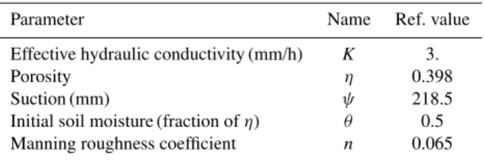
Table 1.Model parameters values derived from soil type and land cover data.
Parameter Name Ref. value Effective hydraulic conductivity (mm/h) K 3.
Porosity η 0.398
Suction (mm) ψ 218.5 Initial soil moisture (fraction ofη) θ 0.5 Manning roughness coefficient n 0.065
Using the values specified in Table 1 (spatially uniform val-ues for model parameters), the resulting specific discharge is typical for Mediterranean flash flood events. The two sub-catchments contributing to the discharge in Labastide-Rouairoux (outlet situated to the north on Fig. 1) are drained by the Thor´e river (eastern part) and the Beson stream (smaller sub-catchment in the western part).
4 Differential sensitivity analysis
In differential sensitivity analysis, first order importance measures are calculated from the gradient when the response is scalar (e.g. peak discharge). For a vectorial response (e.g. entire flood hydrograph), the Jacobian matrix of the trans-formation can be evaluated. It can be computed column by column using the forward mode of AD, line by line using the reverse mode. When the dimension of the parameter space is much larger than the dimension of the response to be anal-ysed, the adjoint technique (e.g. reverse mode of AD) is the most efficient calculation method.
However, using the rate of change along the vectors of the standard basis (components of the gradient), the parameters cannot be ranked because the nominal values might be char-acterised by different units and therefore different orders of magnitude. It is possible to normalize the partial derivatives with the associated nominal values for the parameter and re-sponse (e.g.∂J /∂K.K/¯ J¯). In this case, the importance mea-sure corresponds to the effect on the response from perturb-ing the parameter by a fixed fraction of its base value. In order to take the uncertainty underlying the different param-eters into account, the associated standard deviations (or vari-ance) can be used for the normalization. The resulting impor-tance measure corresponds to the effect on the response from perturbing the parameter by a fixed fraction of its standard deviation (Helton, 1993). Although the approach is quite ap-pealing, this means that derivatives are used for ranking over the space of uncertain parameters. In this paper, the choice was made to prefer a strictly local analysis in which the as-sessment concerns the base point where derivatives are eval-uated.
In the following paragraphs, forward sensitivity analysis will be carried out to a parametrization of reduced dimen-sionality, adjoint sensitivity analysis will be used for the fully
Fig. 1. Ground elevation of the Thor´e basin at Labastide-Rouairoux.
distributed parametrization. In order to facilitate the inter-pretation of the results, a spatially lumped rainfall forcing is used for most of the experiments presented in this section.
4.1 Numerical experiments with network/hillslopes
parametrization
In this paragraph, a classical reduction of the control space is adopted. The drainage network and the hillslopes are dis-tinguished using a threshold on the drained area. It leads to the definition of basis vectors exclusively composed of 0 and 1 on the hillslopes or drainage network. The spatially distributed parameters are expressed in this basis (e.g. rather than the canonical basis). In other words, for each parameter, a scalar multiplier is applied on the hillslopes and another in the drainage network.
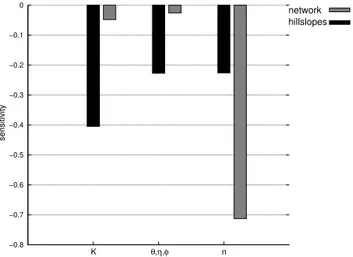
4.1.1 Analysis of a scalar response
The relative importance of the scalar multipliers on two as-pects of the hydrological response (flood volume and flood peak) is provided by Figs. 2 and 3. The parametersθ,ψ andηappear as a product in the infiltration model (Eq. 12). Therefore, given the adopted normalization procedure, they have exactly the same influence on the model response. If a statistical normalization procedure is adopted, the ranking of those parameters would be completely driven by the associ-ated statistical properties (variance or standard deviation).
The analysis of Fig. 2 confirms that the flood volume is mainly driven by the infiltration parameters on the hillslopes (hydraulic conductivityK and initial soil moistureθ). The infiltration parameters assigned on the hillslopes also have a significant influence on the flood peak but the effect of mod-ifying the friction parameter in the drainage network is much larger (see Fig. 3).
The results presented above are strictly local and the im-portance measures are affected by the nominal values as-signed to the different parameters. However, given the re-duced computational cost of the analysis, it can be carried out at different locations in the parameter space. Additional ex-periments (not reported in this paper) where conducted along a transect of the parameter space (θ∈[0,1]). The results show that the wetter the soil at the beginning of the event, the faster the decay of the infiltration rate to the hydraulic conductivity, and therefore the greater the relative influence ofKwhen compared to the initial soil moistureθ.
4.1.2 Analysis of the flood hydrograph
In order to analyse of the effect of parameter variations on the complete flood hydrograph, a vectorial response contain-ing the temporal evolution (80 time steps) of the simulated discharge was considered. Given to the ratio between input and output space dimensions (i.e. 6/80), the Jacobian matrix is computed using the tangent mode of TAPENADE (i.e. for-ward sensitivity analysis).
Each column of the Jacobian matrix represents the varia-tions in discharges resulting from the perturbation of one of the model parameters. After normalization, the physical in-terpretation of the lines and/or columns of the Jacobian ma-trix can provide an interesting insight (not reported in the present contribution). However, a very interesting perspec-tive is provided by the singular value decomposition of this Jacobian matrix.
The singular value decomposition (SVD) of anm×n ma-trixAis a factorization of the form
A=USVT (14)
where S is a diagonal matrix containing the singular val-ues ofAin the decreasing order whileUandVare orthog-onal matrices (respectively of dimensionm×mandn×n). The set of entries composing the main diagonal of S, de-noted
σ1, σ2, . . . , σmin(m,n) , is referred as the singular
spectrum ofA. The columns ofU= {u1,u2, . . . ,um}and
V= {v1,v2, . . . ,vm}are the left and right singular vectors
in the input and output spaces of the transformation repre-sented byA. The magnitude of the singular values inS rep-resents the importance of the corresponding singular vectors in the columns ofUandV.
This factorization is widely used for the analysis of linear ill-posed inverse problems (Hansen, 1998). Its application to non-linear systems can serve many purposes such as sensi-tivity or identifiability analysis, control variables estimation
−0.6 −0.5 −0.4 −0.3 −0.2 −0.1 0
K θ,η,φ n
sensitivity
hillslopes network
Fig. 2. Sensitivity of flood volume to model parameters for net-work/hillslopes parametrization.
−0.8 −0.7 −0.6 −0.5 −0.4 −0.3 −0.2 −0.1 0
K θ,η,φ n
sensitivity
hillslopes network
Fig. 3. Sensitivity of flood peak to model parameters for net-work/hillslopes parametrization.
or perturbations growth analysis in ensemble prediction (Li et al., 2005; Doherty and Randall, 2008; Cl´ement et al., 2004; Marchand et al., 2008; Durbiano, 2001; Buizza and Palmer, 1995).
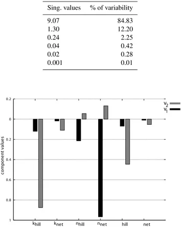
For the adopted network/hillslopes parametrization, the singular spectrum is given by Table 2 and the components of the first 2 singular vectors in the parameter space (right singular vectors) are plotted in Fig. 4. From Table 2, it can be seen that the decay of the singular values is very rapid. Most of the variability (more than 97%) is captured by the first two singular vectors. These vectors exhibit a clear dis-tinction between the production and transfer of runoff. This could have been expected because they represent orthogonal directions in the parameter space.
Table 2. Singular values of the Jacobian matrix for the net-work/hillslopes parametrization.
Sing. values % of variability 9.07 84.83 1.30 12.20 0.24 2.25 0.04 0.42 0.02 0.28 0.001 0.01
1 0.8 0.6 0.4 0.2 0 0.2
khill knet nhill nnet hill net
c
o
m
p
o
n
e
n
t
v
a
lu
e
s
v1 v2
Fig. 4. Components of the first two singular vectors (V1andV2)
of the Jacobian in the parameter space for the network/hillslopes parametrization.
overwhelming influence on the flood hydrograph. The anal-ysis of the second singular vector components indicates a predominance of the hillslopes infiltration parameters and a potential compensation with friction parameters.
Using the adjoint state method (reverse mode of AD) the computational cost related to the evaluation of local sensitiv-ities is not related to the dimension of the parameter space. Therefore a similar analysis was carried out without reduc-tion of the control space using scalar multipliers.
4.2 Numerical experiments with fully distributed
parameters
When no strategy is adopted for dimension reduction, the use of sampling based sensitivity analysis methods is not tractable for distributed parameter systems. In this paragraph the full potential of the adjoint method is exploited in order to analyse the effect on the hydrological response of variations on the value assigned to each element of the computational grid for the model parameters. The analysis is also carried out for a scalar response and for the entire flood hydrograph.
4.2.1 Analysis of a scalar response
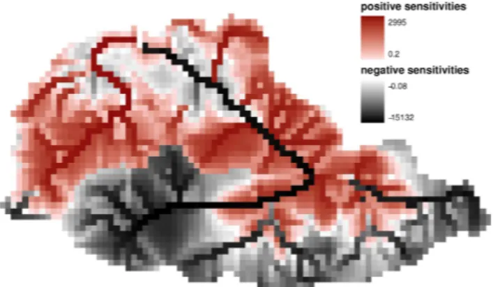
For a scalar response, a single integration of the adjoint model yields to sensitivity indices for all parameters at all spatial locations. In this paragraph, only the sensitivity to the flood peak is reported. Within a single river reach, it is ob-vious that increasing the friction will reduce the maximum discharge (i.e. negative sensitivities at all spatial locations). The situation is more complex when dealing with overland flow over the topography of a catchment.
The analysis of Fig. 5 reveals that positive and negative sensitivities are encountered over the catchment. Negative sensitivities are much larger than positive sensitivities in magnitude but there are locations where increasing the fric-tion coefficient lead to a slight increase of the maximum discharge. While all sensitivities have the expected sign (i.e. negative) along the main stream (i.e. Thor´e river), some positive sensitivities can counterbalance the overall effect in some concomitant sub-basins (e.g. area drained by the Beson stream and some hillslopes along the Thor´e river).
Therefore, when applying a single scalar multiplier for the entire catchment, compensation effects usually occur which are very difficult to identify without such analysis. A simple corroboration can be carried out using multiple model evalu-ations. As an illustration, increasing the nominal by 10% for all roughness coefficients leads to−4.5% variation on the peak discharge. This variation is−5.9% when only the cells featuring a negative sensitivities are modified and it becomes +1.5% when the same operation is carried out on the cells featuring positive sensitivities.
4.2.2 Analysis of the flood hydrograph
When considering the entire flood hydrograph, the ratio be-tween the input and output space dimensions is now very close to 100 (i.e. 3×2582/80). Therefore, the Jacobian ma-trix is computed line by line using multiple integrations of the adjoint model.
In order to facilitate the physical interpretation, the SVD is performed onsub-Jacobians. Eachsub-Jacobianaccounts for a single parameter but for all spatial locations. For a given parameter, the analysis enables an extensive understanding for the influence of the values specified over the entire catch-ment.
encountered when analysing the entire flood hydrograph for both friction coefficient and hydraulic conductivity.
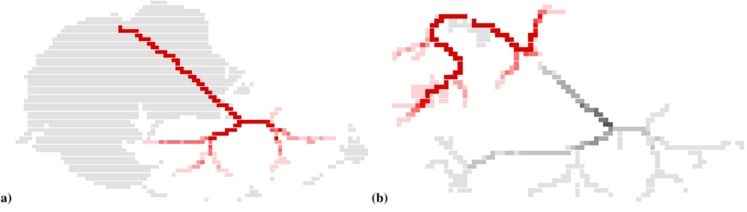
The leading singular vector mainly corresponds to the Thor´e river and drained area for bothnandK(Figs. 6a and 7a). However, the interacting regions are already charac-terised by different signs. For the second singular vectors, the catchment regions and signs are inverted (Figs. 6b and 7b).
The interactions between the two sub-basins can be also analysed in the observation space. For the roughness coef-ficientn, the components ofu1andu2(singular vectors in the observation space) are plotted together with the outlet dis-charge (see Fig. 8). The analysis of this figure explains that the slight disruptions of the hydrograph during both the ris-ing limb and the recession are mainly due to the flood wave coming from the Beson stream. For the imposed spatially lumped rainfall, given that the smaller sub-basin (holdingv2) is closer to the catchment outlet, the resulting smaller con-centration time leads to a quicker response perfectly char-acterised byu2. The correspondence between the singular vectors in the parameter and observation spaces is really in-formative and meaningful.
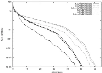
In addition, the singular spectrum for all parameters and different forcing conditions (lumped and spatially variable rainfall) was also analysed. The analysis of Fig. 9 reveals that the decay of singular values is faster for the roughness coefficient when compared to the infiltration parameters. Al-though the influence of friction is very important, less singu-lar vectors are necessary to describe the sub-space producing variability in simulated discharges. This is due to the fact that this subspace is mainly restricted to the drainage network for friction parameters (see Fig. 6).
For a spatially distributed rainfall forcing the decay of sin-gular values appears to be slower and the gap between fric-tion and infiltrafric-tion parameters is reduced. The fact that more singular vectors are necessary to describe the sub-space pro-ducing important variations of the simulated discharges is a sign of increased information content. This increase in in-formation content was expected when comparing the results obtained with uniform rainfall forcing with those obtained for spatially variable precipitations.
It was shown in this section that the derivatives obtained with algorithmic differentiation provide a valuable introspec-tion into the relaintrospec-tion between the model parameters and the simulated hydrological response. The availability of accurate adjoint-based sensitivities also enables the use of efficient gradient-based optimization techniques for the estimation of model parameters.
5 Gradient-based parameter estimation
In this paper, a bound-constrained (inequality constraints) quasi-Newton (BFGS) optimization algorithm (Lemarchal and Panier, 2000) from the MODULOPT library was used.
Fig. 5.Spatial variability for the sensitivity of the flood peak to the friction coefficient.
Using the adjoint sensitivities, the algorithm estimates the active set by performing a Wolfe line search along the gradi-ent projection path.
5.1 Numerical experiments with network/hillslopes
parametrization
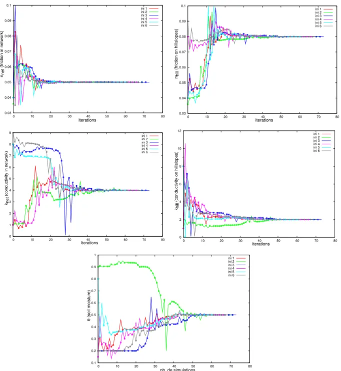
Synthetic observations are generated with the parametriza-tion described in the previous secparametriza-tion withKnet=4mmh−1, Khill=2mmh−1, nnet=0.05, nhill=0.08 and θ=0.5 (uniform over the catchment). The Nash criterion is used to measure the misfit between model simulations and the synthetic ob-servations. As shown in Fig. 10, all control variables are re-trieved independently from the initial parameter values (ini-tial point for the optimization routine). The relative impor-tance of the parameters inferred from the local sensitivity analysis results seems to be similar for the Nash efficiency over the bounded parameter space. The more sensitive is the performance measure to a parameter, the greater is the identi-fiability of this parameter and therefore the faster the iterates convergence to the reference value (e.g. parametersnnetand Khill).
It is important to emphasize that both adjoint (required to the estimation of the gradient) and direct model evalua-tions (required required for the line search) were reported in Fig. 10. The total number of iterations (less than 50) is very small when compared to the number of model evaluations required by evolutionary algorithms like the very popular Shuffled Complex Evolution (SCE) from Duan et al. (1992). As commented by Kavetski et al. (2006), “5 min of Newton computing often replaces 24 h of SCE search and yield useful additional information”.
(a) (b)
Fig. 6. First singular vectors (i.e.(a)v1and (b)v2) in the parameter space for the roughness coefficientn(red color ramp for positive
components and gray for negative).
(a) (b)
Fig. 7. First singular vectors (i.e. (a)v1and(b)v2) in the parameter space for the hydraulic conductivityK(red color ramp for positive
components and gray for negative).
leading singular vectors (i.e. in the parameter space) of the Jacobian matrix. Given that a small number of singular val-ues are dominant, as illustrated in Fig. 9, most of the vari-ability can be captured with very few orthogonal directions in the parameter space. In the following paragraph, the lead-ing slead-ingular vectors of the Jacobian matrix are used in or-der to reduce the dimensionality of the parameter estimation problem.
5.2 Numerical experiments with TSVD
parametrization
Using the sensitivity analysis outcomes, it is possible to carry out parameter estimation in a reduced basis taking the ob-servations information content into account. The spatially distributed model parameters are therefore expressed in the basis spanned by the Jacobian leading singular vectors.
The derivation was carried out at a specific point of the parameter space. However, singular vectors in the param-eter space are mainly dparam-etermined by the topography of the catchment and the spatial variability of rainfall. Important
variations of those orthogonal directions where not encoun-tered when the Jacobian is evaluated at different locations in the parameter space. In order to compute the singular vec-tors describing the relevant sub-space for parameter estima-tion, the SVD was performed for the Jacobian calculated with spatially uniform rainfall forcing. A more rigorous approach would require the Jacobian to be computed with the response of the catchment for several rainfall events.
−1 −0.8 −0.6 −0.4 −0.2 0 0.2
0 10 20 30 40 50 60 70 80 0 50 100 150 200 250
singular vectors components
discharge
time indice
u1 u2
Q(t)
Fig. 8. Singular vector in the observation space for the roughness coefficientn.
The calibration problem is then tackled using tions of increasing dimensionality. The simpler parametriza-tionP1 assigns a single scalar multiplier for each parame-ter over the entire catchment area (i.e.nK=nn=nθ=1 in
Ta-ble 3). ForP2, a scalar multiplier is applied to the hillslopes and another one to the drainage network for the hydraulic conductivity and friction coefficient (i.e.nK=nn=2).
Then, apart from the parameterθ, the number of degrees of freedom is gradually increased by taking as a basis the singular vectors drivingX% of the variability for parameters K andn(parametrizationsPSVXin the table). As reported during the sensitivity analysis (Sect. 4.2.2), the number of degrees of freedom required for the roughness coefficient is much lower than that obtained for the hydraulic conductiv-ity. The number of degrees of freedom for each parameter, the Nash performance for the estimated parameter set and the inverse of the condition number are given in Table 3. The condition number was calculated with an approximation of the hessian after the last BFGS update (i.e. at the optimum) of the quasi-newton algorithm. It is reminded that the larger the ratio 1/κ(H ), the better is the conditioning of the opti-mization problem.
From the results shown in Table 3, it seems that using this description of the parameter space the number of control variables can be increased without altering the conditioning of the optimization problem. The previous statement is valid as long as the vectors describing the kernel in the parameter space (the specified degrees of freedom which do not signif-icantly alter the hydrological response) are not introduced in the parametrization. The results obtained withPSV90 show that even with noise-free observations, the use of those di-rections for the description of the affordable sub-space lead to instability in the inverse problem.
However, it is interesting to note that with respectively 7 and 10 degrees of freedom (i.e. PSV70 and PSV80), the
1e−05 1e−04 0.001 0.01 0.1 1 10 100
0 10 20 30 40 50 60
% of variability
eigenvalues
K (uniform rainfall) n (uniform rainfall)
θ, η, φ (uniform rainfall) K (radar rainfall) n (radar rainfall)
θ, η, φ (radar rainfall)
Fig. 9. Singular values spectrum for lumped and spatially variable rainfall.
Table 3. Complexity (label and number of degrees of freedom for the parametersK,nandθ), Nash efficiency (with synthetic noise free observations) and conditioning for the different parametriza-tions.
nK nn nθ Nash 1/κ(H )
P1 1 1 1 0.908 0.965E-08
P2 2 2 1 0.938 0.217E-11
PSV70 4 2 1 0.968 0.889E-08
PSV80 6 3 1 0.978 0.947E-08
PSV90 9 5 1 0.986 0.242E-16
conditioning is even better than the one obtained with parametrizationP2 (5 degrees of freedom). As emphasised by Tonkin and Doherty (2005), the subspace determined from the truncated singular value decomposition of the Ja-cobian (TSVD) is determined from the observations infor-mation content whereas the subspace constructed from a prior parsimony strategy is not. In the previously cited con-tribution, the Jacobian matrix was approximated using fi-nite differences and used in the linearized equations of the Levenberg-Marquardt method. In order to prevent over-fitting and combine the advantages of TSVD and Tikhonov regularizations an hybrid regularization methodology was proposed.
0.03 0.04 0.05 0.06 0.07 0.08 0.09 0.1
0 10 20 30 40 50 60 70 80
nnet
(friction in network)
iterations
ini 1 ini 2 ini 3 ini 4 ini 5 ini 6
0.03 0.04 0.05 0.06 0.07 0.08 0.09 0.1
0 10 20 30 40 50 60 70 80
nhill
(friction on hillslopes)
iterations
ini 1 ini 2 ini 3 ini 4 ini 5 ini 6
0 1 2 3 4 5 6 7 8 9
0 10 20 30 40 50 60 70 80
knet
(conductivity in network)
iterations
ini 1 ini 2 ini 3 ini 4 ini 5 ini 6
0 2 4 6 8 10 12
0 10 20 30 40 50 60 70 80
khill
(conductivity on hillslopes)
iterations
ini 1 ini 2 ini 3 ini 4 ini 5 ini 6
0.1 0.2 0.3 0.4 0.5 0.6 0.7 0.8 0.9 1
0 10 20 30 40 50 60 70 80
θ
(soil moisture)
nb de simulations
ini 1 ini 2 ini 3 ini 4 ini 5 ini 6
Fig. 10. Convergence of the model parameters to the reference values for various initial parameter sets using quasi-newton algorithm. The displayed iterations contain both gradient calculations with the adjoint (marked with a square) and model evaluations for the line search.
6 Discussion and conclusions
Using a relatively simple application case, it has been shown that the potential of variational methods for distributed catch-ment scale hydrology should be considered. Although for this particular application many outcomes are limited to ev-idence retrieval, the adopted approach should be further ex-ploited.
It is important to emphasise that a single integration of the adjoint code, encompassing the forward integration of the direct model and the backward integration of the adjoint model, yields all spatial and temporal sensitivities (Hall and Cacuci, 1983). The key advantage of this technique is that the computational cost is independent from the dimension of the control space. The results provided in this paper show that spatially distributed parameter sensitivities can be obtained for a very modest calculation effort (∼6 times the comput-ing time of a scomput-ingle model run). The analysis of an essential aspect of the simulated hydrograph such the maximum dis-charge has shown that the influence of the friction coefficient assigned at different spatial locations was characterised by relatively complex sensitivity patterns.
For the analysis of a vectorial response such as the flood hydrograph, the Jacobian of the transformation can be cal-culated using the adjoint technique. The physical interpre-tation of the singular vectors in the parameter and observa-tions spaces brings out relevant features of the rainfall-runoff transformation. Furthermore, the analysis of the singular spectrum can be used to apprehend the complexity of an af-fordable parametrization and compare the information con-tent of different rainfall events. Sensitivity analysis can be motivated by different goals. For understanding the model behaviour for parameter values leading to an acceptable fit to the available observations, the analysis should be carried out with posterior probability distribution functions (PDFs). Us-ing samplUs-ing based approaches, this is rarely the case in prac-tice, partly because posterior PDFs are often characterized by dependence which can be difficult to represent and compro-mise the use of many existing global sensitivity analysis tech-niques (see Kanso et al., 2006 for one of the few attempts). For this specific setting, local sensitivity analysis at the best estimate might prove very informative. Many of the out-comes, such as the spatially distributed importance measures, are mainly driven by the topography of the catchment and the spatial variability of the rainfall forcing rather than the spe-cific point in the parameter space used for the analysis.
For the estimation of model parameters, even when its is obtained with an empirical dimension reduction (e.g. scalar multipliers), uni-modality or at least limited multi-modality can be achieved for many hydrological mod-els. In this case, gradient-based optimization techniques are indisputably the most efficient (i.e. convergence to sin-gle mode or exploration of multi-modality). As under-lined by Kavetski et al. (2006) convergence safeguards such as line-searches and trust-regions in modern gradient-based algorithms improve significantly the reliability of the estimates. The accuracy of the gradient can be es-sential and to this regard, the approach used in this pa-per avoid the specification of a pa-perturbation parameter (re-quired for finite difference approximation). The derivatives computed with the reverse mode of algorithmic differenti-ation (i.e. adjoint method) were found exceedingly efficient in driving a bound-constrained quasi-newton optimization
algorithms to the reference values used to generate synthetic observations.
Although the number of gradient/model evaluations is al-ready eloquent, the authors acknowledge that a comparison with global non-smooth optimization techniques such as the Shuffle Complex Evolution from Duan et al. (1992) would strengthen the argument of the paper. However, the math-ematical representation of hydrological processes in dis-tributed models tend to produce smoother response surfaces. Although the presence of thresholds remains in the model formulations, they usually occur at the grid element level and do not produce discontinuous derivatives for the cost tion. In fact, as far a discharge is concerned, the cost func-tions used for the calibration of model parameters involve an integration of the residuals over time for an integrated hydro-logical response (i.e. spatio-temporal smoothing).
As advocated by Moore and Doherty (2006a,b), empiri-cal dimension reduction do not allow all the information to be extracted from observation data in order to reduce the pre-dictive model error. Parameters at different locations over the surface of the catchment are not equally constrained by the observations of the hydrological response. The identifiable subspace can described using the truncated singular value decomposition of the Jacobian matrix (TSVD). Doherty and Randall (2008) recently proposed statistics for evaluating pa-rameter identifiability and error reduction using this factor-ization of the Jacobian matrix.
The experiments carried out with TSVD parametrization show that this technique represents a promising regulariza-tion strategy. However, as emphasised by Tonkin and Do-herty (2005), it is essential to combine this approach with Tikhonov regularization in order to account for prior infor-mation and prevent overfitting. The appropriate calibration paradigm would therefore require a good compromise to be found between flexibility and stability. The objective would be to improve prior values rather than conducting a blind search over an arbitrarily reduced parameter space.
Acknowledgements. This work was supported by a bi-annual research contract between the Midi-Pyr´en´ees r´egion and the French government funded and managed by the French National Space Agency (CNES). The authors gratefully acknowledge the support of French National Institute for Research in Computer Science and Control (INRIA) and Toulouse Institute of Fluid Mechanics (IMFT).
Edited by: R. Moussa
References
Belanger, E. and Vincent, A.: Data assimilation (4D-VAR) to fore-cast flood in shallow-waters with sediment erosion, J. Hydrol., 300, 114–125, 2005.
Bennett, A.: Inverse Methods in Physical Oceanography, Cam-bridge Monographs on Mechanics and Applied Mathematics, Cambridge University Press, 1992.
Beven, K. and Binley, A.: The future of distributed models : model calibration and predictive uncertainty, Hydrol. Process., 279– 298, 1992.
Bouyssel, F., Cass´e, V., and Pailleux, J.: Variational surface analysis from screen level atmospheric parameters, Tellus A, 51, 453–+, 1999.
Buizza, R. and Palmer, T. N.: The singular vector structure of the global atmospheric global circulation, J. Atmos. Sci., 52, 1434-1456, 1995.
Cacuci, D.: Sensitivity theory for nonlinear systems. I. Nonlinear functional analysis approach, J. Math. Phys., 22(12), 2794–2802, 1981a.
Cacuci, D.: Sensitivity theory for nonlinear systems. II. Extensions to additional classes of responses, J. Math. Phys., 22(12), 2803– 2812, 1981b.
Callies, U., Rhodin, A., and Eppel, D. P.: A case study on varia-tional soil moisture analysis from atmospheric observations, J. Hydrol., 212–213, 95–108, 1998.
Calvet, J.-C., Noilhan, J., and Bessemoulin, P.: Retrieving the Root-Zone Soil Moisture from Surface Soil Moisture or Temperature Estimates: A Feasibility Study Based on Field Measurements, J. Appl. Meteorol., 37, 371–386, 1998.
Carrera, J. and Neuman, S.: Estimation of aquifer parameters under transient and steady state conditions: 2. Uniqueness, stability and solution algorithms, Water Resour. Res., 2, 211–227, 1986. Chavent, G.: Identification of functional parameter in partial
differ-ential equations, in: Identification of Parameters in Distributed Systems, edited by: Goodson R. E., and Polis, M., ASME, New York, 31–48, 1974.
Cl´ement, F., Khvoenkova, N., Cartalade, A., and Montarnal, P.: Analyse de sensibilit´e et estimation de param`etres de transport pour une ´equation de diffusion, approche par ´etat adjoint, INRIA-Rocquencourt, Projet ESTIME, Tech. Rep. RR-5132, 2004. Cukier, R., Levine, H., and Shuler, K.: Nonlinear sensitivity
analy-sis of multiparameter model systems, J. Comput. Phys., 26, 1–42, 1978.
Doherty, J. and Randall, J. H.: Two Statistics for Evaluating Pa-rameter Identifiability and Error Reduction, J. Hydrol., 366(1–4), 119–127, 2009.
Duan, Q., Sorooshian, S., and Gupta, V.: Effective and Efficient Global Optimisation for Conceptual Rainfall-Runoff Models, Water Resour. Res., 28, 1015–1031, 1992.
Durbiano, S.: Vecteurs caract´eristiques de mod`eles oc´eaniques pour la r´eduction d’ordre en assimilation de donn´ees, Ph.D. thesis, Universit´e Joseph Fourier (Grenoble I), 2001.
Estupina-Borrell, V., Dartus, D., and Ababou, R.: Flash flood mod-eling with the MARINE hydrological distributed model, Hydrol. Earth Syst. Sci. Discuss., 3, 3397–3438, 2006,
http://www.hydrol-earth-syst-sci-discuss.net/3/3397/2006/. Ghil, M. and Malanotte-Rizzoli, P.: Data assimilation in
meteorol-ogy and oceanography, Adv. Geophys., 33, 141–226, 1991. Griewank, A.: Evaluating Derivatives: Principles and Techniques of
Algorithmic Differentiation, in: Frontiers in Appl. Math., SIAM,
Philadelphia, PA, Vol. 19, 369 pp., 2000.
Gupta, V. and Sorooshian, H.: The automatic calibration of concep-tual catchment models using derivative based optimization algo-rithms, Water Ressour. Res., 21, 473–485, 1985.
Hall, C. and Cacuci, D.: Physical interpretation of the adjoint func-tions for sensitivity analysis of atmospheric models, J. Atmos. Sci., 40, 2537–2546, 1983.
Hall, J., Tarantola, S., Bates, P., and Horritt, M.: Distributed Sen-sitivity Analysis of Flood Inundation Model Calibration, J. Hy-draul. Eng.-ASCE, 131, 117–126, 2005.
Hansen, P.: Rank-Deficient and Discrete Ill-Posed Problems. Nu-merical Aspects of Linear Inversion, SIAM, Philadelphia, 1998. Hasco¨et, L. and Pascual, V.: TAPENADE 2.1 user’s guide, Tech. Rep. RT-0300, Institut National de Recherche en Informatique et en Automatique (INRIA), 2004.
Helton, J. C.: Uncertainty and sensitivity analysis techniques for use in performance assessment for radioactive waste disposal, Reliab. Eng. Syst. Safe., 42, 327–367, 1993.
Homma, T. and Saltelli, A.: Importance measures in global sensi-tivity analysis of nonlinear models, Reliab. Eng. Syst. Safe., 52, 1–17, 1996.
Honnorat, M., Monnier, J., Lai, X., and Le dimet, F.-X.: Vari-ational data assimilation for 2D fluvial hydraulics simulation, in: CMWR XVI-Computational Methods for Water Ressources, Copenhagen, 2006.
Hornberger, G. and Spear, R.: An approach to the preliminary anal-ysis of environmental systems, J. Environ. Manage.t, 12, 7–18, 1981.
Ibbit, R. and O’Donnell, T.: Designing conceptual catchment mod-els for automatic fitting methods, IAHS Publication, 101, 462– 475, 1971.
Johnston, P. and Pilgrim, D.: Parameter optimization for watershed models, Water Resour. Res., 12, 477–486, 1976.
Kanso, A., Chebbo, G., and Tassin, B.: Application of MCMC-GSA model calibration method to urban runoff quality modeling, Reliab. Eng. Syst. Safe., 91, 1398–1405, 2006.
Kavetski, D., Kuczera, G., and Franks, S. W.: Calibration of con-ceptual hydrological models revisited: 2. Improving optimisation and analysis, J. Hydrol., 320, 187–201, 2006.
Kuczera, G. and Parent, E.: Monte Carlo assessment of parame-ter uncertainty in conceptual catchment models: the Metropolis algorithm, J. Hydrol., 211, 69–85, 1998.
Le Dimet, F.-X. and Talagrand, O.: Variational algorithms for anal-ysis and assimilation of meteorogical observations, Tellus A, 38, 97–110, 1986.
Lemarchal, C. and Panier, E.: Les modules M2QN1 et MQHESS, 2000.
Li, Z., Navon, I., and Hussaini, M. Y.: Analysis of the singular vec-tors of the full-physics Florida State University Global Spectral Model, Tellus A, 57, 560–574, 2005.
Lions, J.: Optimal control of systems governed by partial differen-tial equations, Springer-Verlag, 1968.
Madsen, H.: Parameter estimation in distributed hydrological catch-ment modelling using automatic calibration with multiple objec-tives, Adv. Water Resour., 26, 205–216, 2003.
Marchand, E., Cl´ement, F., Roberts, J. E., and P´epin, G.: Determin-istic sensitivity analysis for a model for flow in porous media, Adv. Water Resour., 31(8), 1025–1037, 2008.
Margulis, S. and Entekhabi, D.: A coupled Land Surface-Boundary Layer Model and its adjoint, J. Hydrometeorol., 2, 274–296, 2001.
McCuen, R.: Component sensitivity: a tool for the analysis of com-plex water resources systems, Water Resour. Res., 9(1), 243–247, 1973a.
McCuen, R.: The role of sensitivity analysis in hydrologic mod-elling., J. Hydrol., 18, 37–53, 1973b.
Moore, C. and Doherty, J.: The cost of uniqueness in groundwater model calibration, Adv. Water Resour., 29, 605–623, 2006a. Moore, C. and Doherty, J.: Role of the calibration process in
re-ducing model predictive error, Water Resour. Res., 41, W05020, doi:10.1029/2004WR003501, 2006b.
Navon, I.: Practical and Theoretical Aspect of Adjoint Parameter Estimation and Identifiability in Meteorology and Oceanogra-phy, Dynam. Atmos. Oceans, 27, 55–79, 1998.
Ngnepieba, P., Le Dimet, F.-X., Boukong, A., and Nguetseng, G.: Inverse problem formulation for parameters determination us-ing the adjoint method, ARIMA Journal – Revue Africaine de la Recherche in Informatique et Math´ematiques Appliqu´ees, 1, 127–157, 2002.
Piasecki, M. and Katopodes, N.: Control of Contaminant Releases in Rivers and Estuaries. Part I: Adjoint Sensitivity Analysis, J. Hydraul. Eng.-ASCE, 123, 486–492, 1997.
Rall, L. B.: Automatic Differentiation: Techniques and Applica-tions. Lecture Notes in Computer Science 120, Springer, Berlin, 1981.
Refsgaard, J.: Parameterisation, calibration and validation of dis-tributed hydrological models, J. Hydrol., 198, 69–97, 1997. Reichle, R., Entekhabi, D., and McLaughlin, D.: Downscaling of
radiobrightness measurements for soil moisture estimation: A four-dimensional variational data assimilation approach, Water Resour. Res., 37(9), 2353–2364, 2001.
Saltelli, A., Chan, K., and Scott, E.: Sensitivity analysis, Wiley series in probability and statistics, Wiley, 2000.
Sei, A. and Symes, W.: A note on consistency and adjointness for numerical schemes, Tech. rep., Department of Computational and Applied Mathematics, Rice University, Tech. Report TR95-04, 1995.
Seo, D., Koren, V., and Cajina, N.: Real-Time Variational Assim-ilation of Hydrologic and Hydrometeorological Data into Oper-ational Hydrologic Forecasting, J. Hydrometeorol., 4, 627–641, 2003a.
Seo, D., Koren, V., and Cajina, N.: Real-time assimilation of radar-based precipitation data and streamflow observations into a dis-tributed hydrologic model, Proceedings of Symposium HS03 held during IUGG2003 at Sapporo, IAHS Publ., 282, 138–142, 2003b.
Singh, V.: Kinematic wave in water ressources: a historical per-spective, Hydrol. Process., 15, 671–706, 2001.
Sirkes, Z. and Tziperman, E.: Finite difference of adjoint or adjoint of finite difference?, Mon. Weather rev., 49, 5–40, 1997. Sobol’, I.: Sensitivity analysis for non-linear mathematical models,
Mathematical Modeling & Computational Experiment, 1, 407-414, 1993 (Engl. transl.).
Sun, N.-Z. and Yeh, W.-G.: Coupled inverse problems in ground-water modeling 1. Sensitivity and parameter identification, Water Resour. Res., 26, 2507–2525, 1990.
Tang, Y., Reed, P., van Werkhoven, K., and Wagener, T.: Advanc-ing the identification and evaluation of distributed rainfall-runoff models using global sensitivity analysis, Water Resour. Res., 43, W06415, doi:10.1029/2006WR005813, 2007a.
Tang, Y., Reed, P., Wagener, T., and van Werkhoven, K.: Comparing sensitivity analysis methods to advance lumped watershed model identification and evaluation, Hydrol. Earth Syst. Sci., 11, 793– 817, 2007b, http://www.hydrol-earth-syst-sci.net/11/793/2007/. Tikhononv, A. N. and Arsenin, V. Y.: Solutions of Ill-posed
Prob-lems, W. H. Winston, Washington, DC, 1977.
Tonkin, M. J. and Doherty, J.: A hybrid regularized inversion methodology for highly parametrized environmental models, Water Resour. Res., 41, W10412, doi:10.1029/2005WR003995, 2005.
Van Werkhoven, K., Wagener, T., Reed, P., and Tang, Y.: Characterization of watershed model behavior across a hy-droclimatic gradient, Water Resour. Res., 44, W01429, doi:10.1029/2007WR0062711, 2008a.
Van Werkhoven, K., Wagener, T., Reed, P., and Tang, Y.: Rainfall characteristics define the value of streamflow observations for distributed watershed model identification, Geophys. Res. Lett., 35, L11403, doi:10.1029/2008GL034162, 2008b.
Vrugt, J. A., Bouten, W., Gupta, H. V., and Sorooshian, S.: Toward improved identifiability of hydrologic model parameters: The information content of experimental data, Water Resour. Res., 38(12), 1312, doi:10.1029/2001WR001118, 2002.
Vrugt, J. A., Gupta, H. V., Bastidas, L. A., Bouten, W., and Sorooshian, S.: Effective and efficient algorithm for multiob-jective optimization of hydrologic models, Water Resour. Res., 39(8), 1214, doi:10.1029/2002WR001746, 2003a.
Vrugt, J. A., Gupta, H. V., Bouten, W., and Sorooshian, S.: A Shuffled Complex Evolution Metropolis algorithm for optimiza-tion and uncertainty assessment of hydrologic model parameters, Water Resour. Res., 39(8), 1201, doi:10.1029/2002WR001642, 2003b.
Wagener, T., McIntyre, N., Lees, M. J., Wheater, H. S., and Gupta, H. V.: Towards reduced uncertainty in conceptual rainfall-runoff modelling: dynamic identifiability analysis, Hydrol. Process., 17, 455–476, 2003.
White, L., Vieux, B., Armand, D., and Le Dimet, F.-X.: Estimation of optimal parameters for a surface hydrology model, Adv. Water Resour., 26(3), 337–348, 2003.
Yapo, P., Gupta, H., and Sorooshian, S.: Multi-objective global op-timization for hydrologic models, J. Hydrol., 204, 83–97, 1997. Yatheendradas, S., Wagener, T., Gupta, H., Unkrich, C., Goodrich,
D., Schaffner, M., and Stewart, A.: Understanding uncertainty in distributed flash flood forecasting for semiarid regions, Water Resour. Res., 44, W05S19, doi:10.1029/2007WR005940, 2008. Zou, X., Navon, I. M., and Sela, J.: Variational data Assimilation