Exact critical values for one-way fixed effects models with random sample sizes

(1)

Contents lists available atScienceDirect

Journal of Computational and Applied

Mathematics

journal homepage:www.elsevier.com/locate/cam

Exact critical values for one-way fixed effects models with

random sample sizes

✩

Célia Nunes

a,

*

, Gilberto Capistrano

b

, Dário Ferreira

a

, Sandra S. Ferreira

a

,

João Tiago Mexia

c

a_{Department of Mathematics and Center of Mathematics and Applications, University of Beira Interior, Covilhã, Portugal} b_{School of Business and Development of Excellence-ENDEX, Pouso Alegre, Brazil}

c_{Center of Mathematics and its Applications, Faculty of Science and Technology, New University of Lisbon, Portugal}

a r t i c l e i n f o

Article history:

Received 18 September 2017

Received in revised form 19 March 2018 MSC: 62J12 62J10 62J99 Keywords: ANOVA

Random sample sizes Fixed effects models Correct critical values Cancer registries

a b s t r a c t

Analysis of variance (ANOVA) is one of the most frequently used statistical analyses in several research areas, namely in medical research. Despite its wide use, it has been applied assuming that sample dimensions are known. In this work we aim to carry out ANOVA like analysis of one-way fixed effects models, to situations where the samples sizes may not be previously known. In these situations it is more appropriate to consider the sample sizes as realizations of independent random variables. This approach must be based on an adequate choice of the distributions of the samples sizes. We assume the Poisson distribution when the occurrence of observations corresponds to a counting process. The Binomial distribution is the proper choice if we have observations failures and there exist an upper bound for the sample sizes. We also show how to carry out our main goal by computing correct critical values. The applicability of the proposed approach is illustrated considering a real data example on cancer registries. The results obtained suggested that false rejections may be avoided by applying our approach.

1. Introduction

Analysis of variance (ANOVA) is one of the most frequently used statistical analyses in practical applications. It is routinely used in several research areas, namely in medical research. Usually, it has been applied assuming that sample dimensions are known. However in many relevant situations we not known beforehand these dimensions. This often occurs when there is a fixed time span for collecting the observations. A motivation example is the collection of data from patients with several pathologies arriving at a hospital during a fixed time period, see e.g. [1,2]. In this work we show how this may be overcome when we carry out ANOVA for one-way fixed effects models.

In these situations it is more appropriate, assuming there are m different levels, to consider the sample sizes as realizations, n1

, . . . ,

nm, of independent random variables, N1

, . . . ,

Nm, [1–6]. By following this methodology we avoid the

assumption of previously known the sample dimensions which renders our approach more realistic.

This new approach must be based on an adequate choice of the distribution of N1

, . . . ,

Nm. These distributions are discrete

with probability points as non negative integers. There are two families of such distributions, according to the non existence or existence of an upper bound for the sample sizes. Starting with no upper bound for the sample sizes we consider that we

✩_{Selected papers of CMMSE-2017, Cadiz, Spain.}

*

Corresponding author.

(2)

have counting processes. Namely we assume that the numbers collected in non overlapping intervals are independent and simultaneous arrivals are not to be expected. We are thus led to consider, possibly non homogeneous, Poisson counting processes. So for fixed collection periods our sample sizes will have Poisson distribution. Going over to the cases with upper bounds for sample sizes we use the Binomial distribution, which would correspond to samples collected in situations when there is a probability p of an observation failing. We assumed this probability to be the same for all treatments.

We are interested in obtaining the critical values for testing the hypothesis

H0

:

µ

1

= · · · =

µ

m

,

which may be rewritten as

H0

:

A

µ =

0

,

(1)

where

µ

is the mean vector of the treatment means with components

µ

1

, . . . , µ

m, and A

= [

Im−1

| −

1m−1

]

, with Icthe c

×

c

identity matrix and 1cthe vector with c components equal to 1.

This paper is structured as follows. Section2considers the two mentioned distributions for the samples sizes. Section3

presents the test statistics and their conditional and unconditional distributions, under the assumption that we have random sample sizes. The presented approach is illustrated through an application on real medical data, using cancer registries, in Section4. In Section5we show how to carry out our main goal by computing correct critical values. Section6presents the results of a simulation study, comparing and relating the performance of our approach with the common ANOVA. We conclude this work in Section7, with some closing remarks.

2. Distributions of the sample sizes

In this section we consider two cases for the distributions of the sample sizes. These will be used to obtain the unconditional distributions of the statistics.

First we will assume that the occurrences of observations correspond to counting processes, leading us to consider the sample sizes, N1

, . . . ,

Nm, as Poisson distributed. Then we will deal with situations when failures may occur on collections

of observations and there exist the upper bounds for the sample sizes, inducing us to consider the Binomial distribution. To avoid the existence of samples without observations and other highly unbalanced cases we assume minimums values for each samples dimension. In previous papers, see e.g. [2,3] and [6], it was only considered a minimum value for the global sample size.

2.1. Counting processes

Let us assume that the occurrence of the observations corresponds to counting processes. An illustrative example of this is the collection of observations during a fixed time period in a study comparing, for example, several pathologies of patients arriving at a hospital. The number of patients for each pathology is not known in advance and the replication of the data collection during a different time period, of the same length, would result in a sample of different size. Another example is the approach presented in [1] where one of the pathologies is rare.

In these situations it is more appropriate to assume that the sample dimensions, N1

, . . . ,

Nm, have Poisson distributions

with parameters

λ

1

, . . . , λ

m. We put Ni

∼

P(

λ

i), i

=

1

, . . . ,

m. Moreover n

=

∑

m

i=1niwill be a realization of the random

variable N

=

m

∑

i=1 Ni

which, given the independence of Ni, i

=

1

, . . . ,

m, N

∼

P

(λ) ,

with

λ = ∑

m_i₌₁

λ

i

.

Furthermore the vector n

=

(n1

, . . . ,

nm)′will be a realization of N

=

(N1

, . . . ,

Nm)′.

For carrying out the inference we will assume that Ni

≥

n•i, i

=

1

, . . . ,

m, which means that we have a minimum

dimension for each sample. In this case the global minimum dimension will be n•

₌

∑

m i=1n • i and n •

₌

(n• 1

, . . . ,

n • m) ′ . So, since we have m different treatments and considering all possible partitions of n into n1

, . . . ,

nm, we take

pn•(n)

=

pr(N

=

n

|

N

≥

n•)

=

n−∑m i=2n • i

∑

n1=n•1

...

n−(∑ℓ−1 i=1ni+ ∑m i=_ℓ+1n • i)

∑

nℓ=n• ℓ

...

n−∑m−1 i=1 ni

∑

nm=n−∑m−1 i=1 ni pr(N

=

n

|

N

≥

n• )

,

ni

=

n • i

, . . . ,

i

=

1

, . . . ,

m

,

(2)

(3)

where, through the independence of Ni, i

=

1

, . . . ,

m, pr(N

=

n

|

N

≥

n•)

=

m

∏

i=1 pr(Ni

=

ni

|

Ni

≥

n • i)

=

m

∏

i=1 pr(Ni

=

ni) pr(Ni

≥

n • i)

=

m

∏

i=1 e−λi₍

λ

ni i

/

ni

!

) 1

−

∑

n • i−1 ui=0 e −λ_i₍

λ

ui i

/

ui

!

)

=

m

∏

i=1

λ

ni i ni

!

(eλi

−

∑

n • i−1 ui=0 λuii ui!)

,

ni

=

n • i

, . . . ,

i

=

1

, . . . ,

m

.

(3) 2.2. Observations failures

Let us now assume there exist upper bounds for the sample sizes, r1

, . . . ,

rm. These upper bounds are not always attained,

since we may have observations failures. This situation may happen for instance when

•

working with patients and, depending on the disease, there is a probability of having incomplete or absent reports;

•

working with grapevines and there is a probability, that may depend on the treatment, some of them wither. In these cases the Binomial distribution is the proper choice. So we assume that the sample dimensions, N1

, . . . ,

Nm, have

Binomial distributions with parameters r1

, . . . ,

rmand 1

−

p, where p denotes the probability of an observation failure. This

probability may be obtained from previous results. We put Ni

∼

B(ri

,

1

−

p), i

=

1

, . . . ,

m. Moreover, according to the

reproducibility of Binomial distributions, we have

N

∼

B

(

r

,

1

−

p

) ,

with r

=

∑

m i=1ri. Assuming that Ni

≥

n • i, i

=

1

, . . . ,

m, and n •

₌

∑

m i=1n •

i, we have pn•(n) as defined in(2), with ni

=

n

• i

, . . . ,

ri

,

i

=

1

, . . . ,

m, where pr(N

=

n

|

N

≥

n• ) is now given by pr(N

=

n

|

N

≥

n•)

=

m

∏

i=1 pr(Ni

=

ni

|

Ni

≥

n • i)

=

m

∏

i=1

(

ri ni

)

(1

−

p)ni_pri−ni

∑

ri ui=n•i pr(Ni

=

ui)

=

m

∏

i=1

(

ri ni

)

(1

−

p)ni_pri−ni

∑

ri ui=n•i

(

ri ui

)

(1

−

p)ui_pri−ui

,

ni

=

n•i

, . . . ,

ri

,

i

=

1

, . . . ,

m

.

(4)

3. Test statistic and their conditional and unconditional distributions

In this section, we start by presenting the test statistic and their conditional distribution (assuming fixed sample sizes). Then we will obtain the unconditional distribution, under the assumption that we have random sample sizes.

When Ni

=

ni, i

=

1

, . . . ,

m, we have the samples Yi,1

, . . . ,

Yi,ni

,

i

=

1

, . . . ,

m

,

with averages Yi,•, i

=

1

, . . . ,

m.

Assuming that the observations are normal and independent with variance

σ

2, when Ni

=

ni, i

=

1

, . . . ,

m, the vector of

treatment means, Y•, which has components Y1,•

, . . . ,

Ym,•, will be normal with mean vector

µ

and variance–covariance

matrix

σ

2_D(1 n1

, . . . ,

1 nm), where D( 1 n1

, . . . ,

1

nm) is the diagonal matrix with principal elements

1

n1

, . . . ,

1

nm.

So, when Ni

=

ni, i

=

1

, . . . ,

m, see for instance [7,8], the sum of squares for testing the null hypothesis, H0

:

A

µ =

0,

will be Snum

=

(AY•) ′

(

AD

(

1 n1

, . . . ,

1 nm

)

A′

)

−1 (AY•)

,

(5)

which corresponds to the product by

σ

2_{of a noncentral chi-square with g}

₌

_m

₋

_{1 degrees of freedom and non-centrality}

parameter

δ

(n)

=

1

σ

2(A

µ

) ′

(

AD

(

1 n1

, . . . ,

1 nm

)

A′

)

−1 (A

µ

)

,

(6) Snum

∼

σ

2

χ

g2,δ(n).

(4)

The sum of the sums for the error will be given by, see e.g. [9] and [10], S

=

m

∑

i=1 ni

∑

k=1 (Yi,k

−

Yi,•)2

.

Moreover S will be the product by

σ

2_{of a central chi-square with}

g(n)

=

n

−

m

degrees of freedom, S

∼

σ

2

χ

_g(n)2 , and will be conditionally independent from Snum.

Therefore, when N

=

n, the conditional distribution of

ℑ =

Snum

S (7)

will be a noncentral F distribution, which corresponds to the distribution of the quotient of independent chi-squares with g and g(n) degrees of freedom and non-centrality parameters

δ

(n) and 0, denoted by F (

.|

g

,

g(n)

, δ

(n)).

Moreover, using the mixtures method of Robbins [11] and Robbins and Pitman [12] (see also [13]),

F (z

|

g

,

g(n)

, δ

(n))

=

e−δ(n)/2 ∞

∑

i=0

δ

(n)i 2i_i

_!

F (z

|

g

+

2i

,

g(n))

,

which corresponds to the distribution of the test statistic when the sample sizes are n1

, . . . ,

nm.

Given N

=

n, when H0holds,

δ

(n)

=

0 and the conditional distribution of

ℑ

will be a central F distribution with g and

g(n) degrees of freedom, F (z

|

g

,

g(n)).

Assuming that the occurrences of the observations corresponds to counting processes, when H0holds the unconditional

distribution of

ℑ

, defined by(7), will be given by, see e.g. [2] and [3],

F (z)

=

∞

∑

n=n• pr(N

=

n

|

N

≥

n•)F (z

|

g

,

g(n))

=

∞

∑

n=n• pn•(n)F (z

|

g

,

g(n))

,

(8) considering pn•(n) as defined in(2).

When we know that N

≤

n, we may not consider in(8)the terms for n

>

n

,

and we have F (z) bounded by

Fn(z)

≤

F (z)

≤

F ∗ n(z)

,

(9) where Fn(z)

=

n

∑

n=n• pr(N

=

n

|

N

≥

n• )F (z

|

g

,

g(n)) (10) and F ∗ n(z)

=

Fn(z)

+

∞

∑

n=n+1 pr(N

=

n

|

N

≥

n•)

.

(11)

So n denotes the upper bound needed to control the truncation error of the unconditional distribution F (z). It is important to note that ∞

∑

n=n+1 pr(N

=

n

|

N

≥

n•)

=

1

−

n

∑

n=n• pr(N

=

n

|

N

≥

n•)

.

(12)

Let us now consider the noncentral distributions. As we saw, when N

=

n

,

Snum

∼

σ

2

χ

g2,δ(n), thus we have

ℑ ∼

F (z

|

g

,

g(n)

, δ

(n))

,

and the corresponding unconditional distribution is given by

F ◦ (z)

=

∞

∑

n=n• pr(N

=

n

|

N

≥

n•)F (z

|

g

,

g(n)

, δ

(n))

.

So we have F ◦ n(z)

≤

F ◦ (z)

≤

F ◦∗ n (z)

,

(5)

Table 1

Number of patients and sample means.

Type of cancer Number of patients Sample means Soft tissues of the thorax 18 49.5000

Intestinal tract 22 61.7727 Nasal cavity 25 62.4000 with F ◦ n(z)

=

n

∑

n=n• pr(N

=

n

|

N

≥

n•)F (z

|

g

,

g(n)

, δ

(n)) and F ◦∗ n (z)

=

F ◦ n(z)

+

∞

∑

n=n+1 pr(N

=

n

|

N

≥

n•)

.

Let us note that

F ◦∗ n (z)

−

F ◦ n(z)

=

F ∗ n(z)

−

Fn(z)

=

∞

∑

n=n+1 pr(N

=

n

|

N

≥

n•)

,

so we may use the same value n that was used for the central case.

3.2. Observations failures

Assuming that we have the upper bounds for the sample sizes, r1

, . . . ,

rm, which are not always attained since failures

may occur, the unconditional distribution of

ℑ

, when H0holds, will be given by

F (z)

=

r

∑

n=n• pr(N

=

n

|

N

≥

n• )F (z

|

g

,

g(n))

=

r

∑

|

g

,

g(n))

,

(13) with r

=

∑

m

i=1riand pn•(n) as defined in(2), where in this case ni

=

n•i

, . . . ,

ri

,

i

=

1

, . . . ,

m. 4. Application

In this section we evaluate our approach under a real data example. To construct this experiment we resort to a dataset which was provided by the Brazilian National Cancer Institute (INCA) [14]. The dataset gathers information regarding the age of patients with cancer disease. The data considered is from 2010 and refers to the City of São Paulo, Brazil.

Two situations will be considered, first assuming that the entries in the samples correspond to independent counting processes and then assuming that we may have observations failures.

All computational procedures, namely the quantiles of the conditional and unconditional distribution as well as all the computations in Sections5and6, were performed using R software.

In our model the factor considered is the Type of Cancer, with three levels: Soft tissues of the thorax, Intestinal tract and Nasal

cavity.Tables A.1–A.3inAppendixshow the frequencies of these three types of cancers, grouped by age.Table 1illustrates

the number of patients and the sample mean age for each type of cancer. We will test the hypothesis

H0

:

A

µ =

0

,

with A

=

[

1 0

−

1 0 1

−

1

]

.

The numerator of the

ℑ

statistic is now given by

Snum

=

(AY•) ′

(

AD

(

1 18

,

1 22

,

1 25

)

A′

)

−1 (AY•)

,

which is, when H0holds, the product by

σ

2of a central chi-square with g

=

m

−

1

=

2 degrees of freedom, Snum

∼

σ

2

χ

22.

So, we obtain

(

AD

(

1 18

,

1 22

,

1 25

)

A′

)

−1

=

[

13

.

0154

−

6

.

0923

−

6

.

0923 14

.

5538

]

and Ay•

=

[−

12

.

9000

−

0

.

6273

]

,

(6)

Table 2

The quantiles of the conditional distribution.

Values ofα 0.1 0.05 0.01

z1−α 0.07711 0.10146 0.16016

where y•has components y_1,•

=

49

.

5000

;

y_2,•

=

61

.

7727

;

y_3,•

=

62

.

4000. Therefore for the numerator of the statistic we

obtain

Snum

=

2073

.

021

.

The denominator of the statistic is, when N

=

n, the product by

σ

2_{of a central chi-square with g(n)}

₌

_n

₋

_{3 degrees of}

freedom, S

∼

σ

2

χ

_n2₋₃. In this case we obtain

S

=

18

∑

j=1 (y_1,j

−

y1,•)2

+

22

∑

j=1 (y_2,j

−

y2,•)2

+

25

∑

j=1 (y_3,j

−

y3,•)2

=

26632

.

364

.

So, the statistic’s value,

ℑ

_Obs, is given by

ℑ

_Obs

=

2073

.

021

26632

.

364

=

0

.

07784

.

Given N

=

n, when H0 holds, the common conditional distribution of

ℑ

is a central F distribution with g

=

2 and

g(n)

=

65

−

3

=

62 degrees of freedom, since n

=

65, F (z

|

2

,

62)

.

The quantiles, z1−α, of the conditional distribution are given inTable 2. These quantiles are obtained considering zα

=

2

62f1−α,2,62, where f1−α,2,62corresponds to the 1

−

α

quantile of a central F distribution with 2 and 62 degrees of freedom.

So we can conclude that using the common approach we reject H0for

α =

0

.

1, since

ℑ

Obs

>

z1−_α, and we do not reject for

α =

0

.

05 and 0.01.

To carry out the computation we are led to use our previous information assuming that

λ

i

,

i

=

1

,

2

,

3 correspond to the

average numbers of occurrences per year. So we take

λ

1

=

18

;

λ

2

=

22 and

λ

3

=

25, which means that N1

∼

P(18),

N2

∼

P(22) and N3

∼

P(25). Let us also assume that we have at least 5 observations per level, which means that

n•_i

=

5

,

i

=

1

,

2

,

3

,

n•

=

∑

3

i=1ni

=

15 and consequently n

•

=

(5

,

5

,

5)′

.

To compute the quantiles for the unconditional distribution we obtain the minimum value n

=

97 (considering in expression(10)) such that

∞

∑

n=n+1 pr(N

=

n

|

N

≥

n•)

=

1

−

n

∑

n=n• pr(N

=

n

|

N

≥

n•)

<

10−4

.

(14)

Therefore, the infinite series in(8)is truncated not considering the terms for n

>

97. So, when H0 holds, we have the

distribution Fn(z)

=

97

∑

n=15 pn•(n)F (z

|

2

,

n

−

3)

=

97

∑

n=15 n−10

∑

n1=5 n−(n1+5)

∑

n2=5 n−(n1+n2)

∑

n3=n−(n1+n2) pr(N

=

n

|

N

≥

n•)F (z

|

2

,

n

−

3)

,

with pr(N

=

n

|

N

≥

n•)

=

3

∏

i=1

λ

ni i

/

ni

!

eλi

−

∑

4 ui=0 λui i ui!

.

The quantiles, z₁t−α

,

for the probability 1

−

α

, of this distribution are presented inTable 3. Since

ℑ

Obs

<

zt1−α

,

we can

conclude that we do not reject H0for the usual level of significance. So these results lead us to take a contrary decision that

(7)

Table 3

The quantiles of the unconditional distribution (counting processes).

Values ofα 0.1 0.05 0.01

zt

1−α 0.07856 0.10341 0.16341

4.2. Observations failures

To carry out the computations we use our previous information assuming that the probability of a failure is equal to 0.2 (p

=

0

.

2). Therefore the probability of collecting a designed observation may be taken as 1

−

p

=

0

.

8, i

=

1

,

2

,

3, and consequently r1

=

22, r2

=

27 and r3

=

31 (sincen_ri_i

≃

1

−

p, i

=

1

,

2

,

3). This means that N1

∼

B(22

,

0

.

8), N2

∼

B(27

,

0

.

8)

and N3

∼

B(31

,

0

.

8). According to the reproducibility of Binomial distributions we will have N

∼

B(80

,

0

.

8).

Let us assume, as before, that we have at least 5 observations per level, so n•_i

=

5, i

=

1

,

2

,

3, n•

=

(5

,

5

,

5)′and n•

=

15. Therefore we have F (z)

=

80

∑

n=15 pn•(n)F (z

|

2

,

n

−

3)

=

80

∑

n=15 n−10

∑

n1=5 n−(n1+5)

∑

n2=5 n−(n1+n2)

∑

n3=n−(n1+n2) pr(N

=

n

|

N

≥

n• )F (z

|

2

,

n

−

3)

,

with pr(N

=

n

|

N

≥

n•)

=

3

∏

i=1

(

ri ni

)

0

.

8ni₀

.

₂ri−ni

∑

ri ui=5

(

ri ui

)

0

.

8ui₀

.

₂ri−ui

.

The obtained quantiles, zb

1−α, for probability 1

−

α

of this distribution, are presented inTable 4. We conclude that we do

not reject H0for the usual levels of significance, which agree with the counting processes’s results. Table 4

The quantiles of the unconditional distribution (observations failures).

Values ofα 0.1 0.05 0.01

zb

1−α 0.07871 0.10361 0.16365

In summary, we draw the following conclusions: The classical F -tests provide quantiles that are slightly smaller than the ones given by the unconditional approach, leading us to take a contrary decision for

α =

0

.

1. Therefore the proposed methodology, beyond being more realistic when the sample sizes are unknown, gives more precise critical values leading to a decrease in the probability of false rejections.

5. Computing critical values

This section presents a new way to compute correct critical values, which may be important to avoid working with incorrect test levels. We assume that the occurrence of observations corresponds to counting processes.

As previously shown in Section3.1,

F (z)

=

∞

∑

n=n• pr(N

=

n

|

N

≥

n• )F (z

|

g

,

g(n))

=

∞

∑

|

g

,

g(n))

,

with pn•(n) as defined in(2).

So, throught(9)we have

Fn(z)

≤

F (z)

≤

F

∗

n(z)

,

and consequently

f_n∗_,1−α

<

f1−α

<

fn,1−α

,

with fn,1−α, f1−αand f_n∗_,1−αthe (1

−

α

)th quantiles for these distributions, see [3].

Therefore, the approximate quantile value can be taken by

˜

f1−α

=

fn,1−α

+

f_n∗_,₁₋_α

(8)

which can be used as a critical value for the usual values of

α

, see [2].

5.1. Computing lower bounds for Poisson parameters

Since the parameters

λ

i, i

=

1

, . . . ,

m, are unknown, we now show how to deal with them in order to compute the critical

values.

Nunes et al. [2] showed that the unconditional distribution increases with

λ

i, i

=

1

, . . . ,

m. Therefore the corresponding

quantiles decrease and we will use lower bounds for these parameters. The lower bounds will be the minimum values of

λ

i, i

=

1

, . . . ,

m, such that

e−λi

λ

ni i

ni

!

=

α,

i

=

1

, . . . ,

m

,

(16)

with

α

the usual level of significance. So, considering gni(

λ

i)

=

1 ni

!

e−λi

λ

ni i

,

we obtain dgni(

λ

i) d

λ

i

= −

1 ni

!

e−λi

λ

ni i

+

1 ni

!

e−λi_n i

λ

ni−1 i

=

1 ni

!

e−λi

λ

ni−1 i (

−

λ

i

+

ni)

,

which means that gni(

λ

i) increases with

λ

i, when

λ

i

<

ni, i

=

1

, . . . ,

m. Therefore we will work with the left solution,

λ

α,i,

of Eq.(16)to obtain the (1

−

α

)% confidence interval for

λ

i, i

=

1

, . . . ,

m,

[

λ

_α,_i

; +∞[

.

Table 5

The lower bounds forλi, i=1,2,3.

Values ofα 0.05 0.01

λα,1 13.5 10.5

λα,2 17.5 13.75

λα,3 20.5 16.25

5.2. Computation results

In order to compute the critical values we consider that ni, i

=

1

,

2

,

3, corresponds to the number of patients presented

inTable 1. We also assume that we have the same minimum dimension for each sample (n•

i

=

5

,

i

=

1

,

2

,

3).

The obtained lower bounds,

λ

_α,i, for the

λ

i, i

=

1

,

2

,

3, considering

α =

0

.

05 and

α =

0

.

01, are presented inTable 5.

Resorting to(10), we have Fn(z)

=

n

∑

n=15 pn•(n)F (z

|

2

,

n

−

3) and F ∗ n(z)

=

Fn(z)

+

(

1

−

n

∑

n=15 pn•(n)

)

=

Fn(z)

+

q

,

where q

=

1

−

n

∑

n=15 pn•(n)

,

which do not depend on z. Assuming the lower bounds for

λ

i, i

=

1

,

2

,

3 we obtained the minimum value n

=

80 [n

=

66]

such that q

<

10−4_for

_{α =}

₀

_.

_{05 [}

_{α =}

₀

_.

_{01]. We computed the quantiles of F}∗

n(z) replacing 1

−

α

by (1

−

α

)

−

q, assuming

that q

=

10−4.

The obtained critical values,

˜

f1−α, defined in(15), are presented inTable 6.

Comparing these critical values with those obtained in Section4.1we find that these ones are slightly higher than the previous ones. This appears to be a reasonable ‘‘price’’ for the increase of robustness due to use of a more complete model (obtained with the estimation of the parameters

λ

i, i

=

1

, . . . ,

m instead of assuming their values). Moreover the use of

(9)

Table 6

Correct critical values.

Values ofα 0.05 0.01

˜f1−α 0.13476 0.28704

6. A simulation study

In this section we carry out a simulation study to compare and relate the performances of our approach with those of common ANOVA.

In these simulations we considered three sets of values for

λ

1,

λ

2and

λ

3. These sets are presented inTable 7. For each

λ

i, i

=

1

,

2

,

3, in each set we generated a Poisson distributed sample with size 30. Thus for each set of

λ

i, i

=

1

,

2

,

3, we had

30 triplets of sample sizes from which we obtained the corresponding conditional critical values as well as lower bounds for the Poisson parameters (which correspond to the left solution of Eq.(16)), both for a 5% level. Assuming to have at least 5 observations per level and n such that the truncation errors do not exceed 10−4_{we also obtained the 5% unconditional}

critical values for each sample triplets. The minimum value of n for each set of

λ

i, i

=

1

,

2

,

3, presented inTable 7, allows us

to conclude that we have a good control of the truncation error.

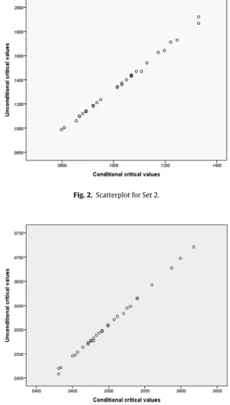
Thus for each initial sets of parameters values we had, also at 5% level, 30 pairs for conditional and unconditional critical values. These pairs are shown inFigs. 1–3. We see that there is a close linear relation between conditional and unconditional critical values, which is confirmed by the Pearson correlation coefficients presented inTable 7.

The close relation points the possibility of estimating unconditional critical values from the conditional ones using the empirical regression, whose equations are presented also inTable 7, where y denotes the unconditional and x the conditional critical values. We also checked that the assumptions underlying the analysis of residues for the adjusted linear regressions did hold.

Table 7

Simulation results.

λ1 λ2 λ3 Minimum n Correlation coefficient Empirical regressions

Set 1 9 11 13 55 0.995 y=0.079+1.13x

Set 2 18 22 25 100 0.999 y= −0.038+1.704x

Set 3 36 44 50 184 0.999 y= −0.012+1.363x

Fig. 1. Scatterplot for Set 1. 7. Closing remarks

In this paper we propose to assume the sample sizes as realizations of random variables when they are not known in advance. In light of this we were able to obtain precise critical values, thus overcoming the fact that using the usual approach only approximate critical values may be obtained when the sample dimensions are unknown. To conduct our approach we resorted to the Poisson and Binomial distributions as the adequate choices for the distributions of the sample sizes. We open room to a new field based on the assumption that we have a minimum dimension for each sample considering one-way ANOVA. Through the application presented we can confirm that the quantiles may exceed those of the common ANOVA

(10)

Fig. 2. Scatterplot for Set 2.

Fig. 3. Scatterplot for Set 3.

when random sample sizes are considered, giving relevance to the unconditional approach in avoiding false rejections. We showed how to obtain correct critical values, giving us the possibility to carry out tests with proper level. In Section6we conclude there exists a close linear relation between conditional and unconditional critical values. We intend to deepen the study in a future work and check the possibility of estimating the unconditional critical values from the conditional ones.

In our approach we worked with F instead of F distribution, since F leads to useful monotony properties that lighten the treatment.

Acknowledgments

The authors would like to thank the anonymous referees for useful comments and suggestions. This work was partially supported by national funds of FCT —Foundation for Science and Technology, Portugal under UID/MAT/00212/2013 and UID/MAT/00297/2013.

Appendix. Frequency tables of types of cancers

(11)

Table A.1

Soft tissues of the thorax cancer.

Ages 1–4 5–9 10–14 15–19 20–24 25–29 30–34 35–39 40–44 Mean age 2 7 12 17 22 27 32 37 42 Patients 0 0 0 2 1 2 1 1 2 Ages 45–49 50–54 55–59 60–64 65–69 70–74 75–79 80–84 85+ Mean age 47 52 57 62 67 72 77 82 87 Patients 2 0 0 0 2 1 1 2 1 Table A.2

Intestinal tract cancer.

Ages 1–4 5–9 10–14 15–19 20–24 25–29 30–34 35–39 40–44 Mean age 2 7 12 17 22 27 32 37 42 Patients 0 0 0 0 0 1 1 1 0 Ages 45–49 50–54 55–59 60–64 65–69 70–74 75–79 80–84 85+ Mean age 47 52 57 62 67 72 77 82 87 Patients 3 3 2 1 3 0 1 2 4 Table A.3 Nasal cavity cancer.

Ages 1–4 5–9 10–14 15–19 20–24 25–29 30–34 35–39 40–44 Mean age 2 7 12 17 22 27 32 37 42 Patients 0 0 0 1 1 0 0 2 0 Ages 45–49 50–54 55–59 60–64 65–69 70–74 75–79 80–84 85+ Mean age 47 52 57 62 67 72 77 82 87 Patients 1 4 0 4 1 3 3 1 4 References

[1] C. Nunes, D. Ferreira, S.S. Ferreira, J.T. Mexia, F -tests with a rare pathology, J. Appl. Stat. 39 (3) (2012) 551–561.http://dx.doi.org/10.1080/02664763. 2011.603293.

[2] C. Nunes, D. Ferreira, S.S. Ferreira, J.T. Mexia, Fixed effects ANOVA: an extension to samples with random size, J. Stat. Comput. Simul. 84 (11) (2014) 2316–2328.http://dx.doi.org/10.1080/00949655.2013.791293.

[3] J.T. Mexia, C. Nunes, D. Ferreira, S.S. Ferreira, E. Moreira, Orthogonal fixed effects ANOVA with random sample sizes, in: Proceedings of the 5th International Conference on Applied Mathematics, Simulation, Modelling (ASM’11), 2011, pp. 84–90..

[4] E.E. Moreira, J.T. Mexia, C.E. Minder, F tests with random sample size. Theory and applications, Stat. Probab. Lett. 83 (6) (2013) 1520–1526.http: //dx.doi.org/10.1016/j.spl.2013.02.020.

[5] C. Nunes, G. Capistrano, D. Ferreira, S.S. Ferreira, J.T. Mexia, One-way fixed effects ANOVA with missing observations, in: Proceedings of the 12th International Conference on Numerical Analysis and Applied Mathematics, in: AIP Conf. Proc., vol. 1648, 2015, 110008.http://dx.doi.org/10.1063/1. 4912415.

[6] G. Capistrano, C. Nunes, D. Ferreira, S.S. Ferreira, J.T. Mexia, One-way random effects ANOVA with random sample sizes: An application to a brazilian database on cancer registries, in: Proceedings of the 12th International Conference on Numerical Analysis and Applied Mathematics, in: AIP Conf. Proc., vol. 1648, 2015, 110009.http://dx.doi.org/10.1063/1.4912416.

[7]E.L. Lehmann, Testing Statistical Hypotheses, John Wiley & Sons, Inc., New York, 1959.

[8]J.T. Mexia, Best linear unbiased estimates, duality of F tests and the Scheffé multiple comparison method in presence of controled heterocedasticity, Comput. Statist. Data Anal. 10 (3) (1990) 271–281.

[9]A.I. Khuri, T. Mathew, B.K. Sinha, Statistical Tests for Mixed Linear Models, in: Wiley series in Probability and Statistics, John Wiley & Sons, New York, 1998.

[10]S.R. Searle, G. Casella, C.E. McCulloch, Variance Components, in: Wiley series in Probability and statistics, John Wiley & Sons, New York, 1992. [11]H. Robbins, Mixture of distribution, Ann. Math. Stat. 19 (1948) 360–369.

[12]H. Robbins, E.J.G. Pitman, Application of the method of mixtures to quadratic forms in normal variates, Ann. Math. Stat. 20 (1949) 552–560. [13] C. Nunes, D. Ferreira, S.S. Ferreira, J.T. Mexia, Control of the truncation errors for generalized F distributions, J. Stat. Comput. Simul. 82 (2) (2012)

165–171.http://dx.doi.org/10.1080/00949655.2011.631924.