Empirical models for grape vine leaf area estimation on cv. Trincadeira

(1)

Master of Science in Viticulture & Enology

Joint diploma “EuroMaster Vinifera” awarded by:

I

NSTITUT

N

ATIONAL D

'

ETUDES SUPERIEURES AGRONOMIQUES DE

M

ONTPELLIER

AND

I

NSTITUTO

S

UPERIOR DE

A

GRONOMIA DA

U

NIVERSIDADE DE

L

ISBOA

Master thesis

Empirical Models for Grape vine Leaf Area Estimation on cv. Trincadeira

Tobias WInkler

2014-2016

supervisor: Prof. Dr. Carlos Manuel Antunes LOPES, ISA Lisbon

supervisor: Prof. Dr. Jorge Filipe Campinos Landerset CADIMA, ISA Lisbon

Jury:

President: - Augusto Manuel Nogueira Gomes Correia (Phd), Associated Professor with aggregation at Instituto Superior de Agronomia, Universidade de Lisboa.

Members: - Hans-Reiner Schultz (Phd) Professor at Geisenheim University;

- Pedro Jorge Cravo Aguiar Pinto (Phd), Full Professor, at Instituto Superior de

Agronomia, Universidade de Lisboa;

- Jorge Filipe Campino Landerset Cadima (Phd), Associated Professor at Instituto

Superior de Agronomia, Universidade de Lisboa, supervisor

(2)

Acknowledgements

.

I would like to thank Professors Carlos Manuel Antunes Lopes and Jorge Filipe Campinos Landerset Cadima for their invaluable consultation regarding viticulture and statistics throughout the writing of this thesis, João Graça and Ricardo Egipto for providing the dataset of 2015 and the support in the used methodologies and Lorenza Bazzano and Helena Horvat for their patient help with the laboratory work. My biggest gratitude goes to my family who encouraged my decision to apply for the Vinifera Euromaster and supported me in so many ways during my life. Finally, I am thankful for the scholarship of Erasmus Mundus Program, without which my Master studies would not have been possible.

This research has received funding from the European Community’s Seventh Framework Programme (SME 2013-2), grant agreement nº 605630, Project VINBOT.

(3)

I

List of Figures

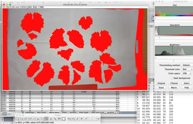
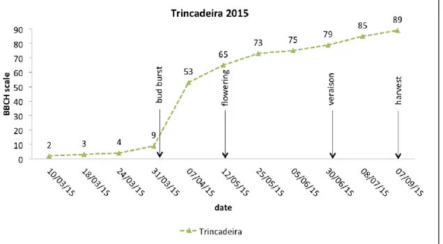
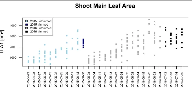
Figure 1: Interface of ImageJ version 1.50g (Wayne Rasband, National Institute of Health, USA), using a hue, saturation and brightness threshold method for Leaf Area assessment. Segmented Leaves are highlighted from the background and LA is measured, using a reference scale (bottom). ... 23 Figure 2: phenological development (BBCH-scale) of Trincadeira during growing season 2015 ... 27 Figure 3: phenological development (BBCH-scale) of Trincadeira during growing season 2016, red line represents vegetative organs, blue line represents reproductive organs ... 27 Figure 4: Shoot Main Leaf Area (TLA1) in cm2_{, plotted by sampling date in two consecutive years 2015}

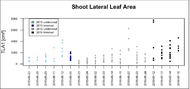
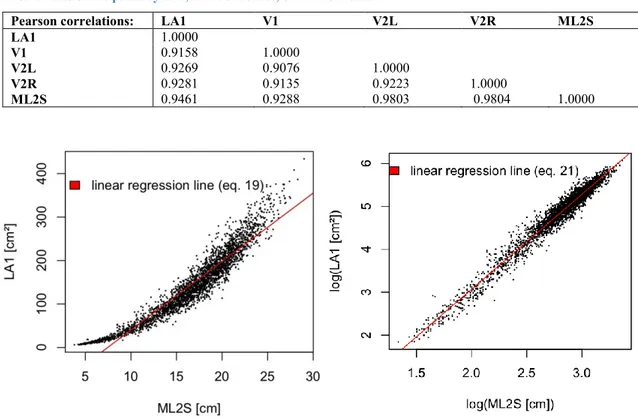
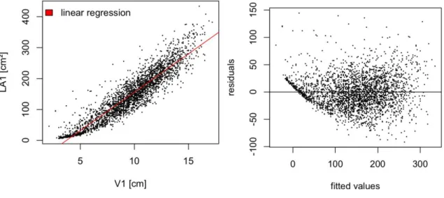
(blue boxes) and 2016 (grey boxes)... 28 Figure 5: Shoot Lateral Leaf Area (TLA2) in cm2, plotted by sampling date for the consecutive years 2015 (blue boxes) and 2016 (grey boxes) ... 29 Figure 6: scatterplots of LA1 as response variable and sum of lateral veins of primary leaves (ML2S) as predictor variable; on the left showing strong curvature of untransformed variables, and without curvature on the right, with linear relation of transformed variables ... 30 Figure 7: Leaf Area LA1 vs. central vein length (V1) (left), showing curvature; on the right residuals vs. fitted plot, with obvious curvature of residuals, strong underestimation in extreme values and

overestimation in medium values ... 32 Figure 8: single primary leaf area (LA1) over central vein length (V1) with both power functions, by nonlinear regression (eq. 16) and transformation (eq. 18) ... 33 Figure 9: Plot of values of single primary leaf area (LA1) versus sum of lateral vein lengths (ML2S). With both regression lines: equation 20 (red) and equation 22 (green) ... 37 Figure 10: scatterplot of single lateral leaf area (LA2) and sum of lateral vein lengths, with power law functions predicted by nonlinear regression (equation 28) and linear regression of logarithmic transformed values (equation 30) ... 41 Figure 11: Transformed variables of Leaf area (log(LA)) over sum of lateral vein lengths (log(V2S)), with lateral and primary leaves estimated by general and type-specific models ... 43 Figure 12: Shoot Primary Leaf Area (TLA1) over Shoot Area (STA), by groups of trimmed and

untrimmed shoots, with regression line of equation 35 ... 49 Figure 14: Shoot Primary leaf Area (TLA1) over Mean Primary Leaf Area (MLA1) with regression lines of presented power models (equation 39 and 41) and the power model (equation 37) presented by Lopes and Pinto (2005) ... 52 Figure 15: estimation of TLA2 by NL2 with 3rd degree polynomial model (equation 41) and power model (equation 42) ... 55 Figure 16: Observed vs. Estimated Shoot Lateral Leaf Area; on the left with simple and multi linear regression of equations 46 and 49, on the right with simple and multi linear regression of transformed variables of equations 47 and 50 ... 59

(6)

IV

Figure 17: scatterplot of single lateral leaf area (LA2) vs. central vein length (V1), with regression line (equation 23) ... 69 Figure 18: scatterplot od single lateral leaf area (LA2) vs. central vein length (V1) with regression lines of equations 24 (nonlinear regression) and 26 (transformed variables ... 70 Figure 19: dependent vs. independent variable and regression line with equation 43: TLA=

0.02967*STA^2.2993; left side untransformed scales, right sight logarithmically transformed scales. Well visible the poor prediction of extreme big TLA2 ... 72

(7)

V

List of Tables

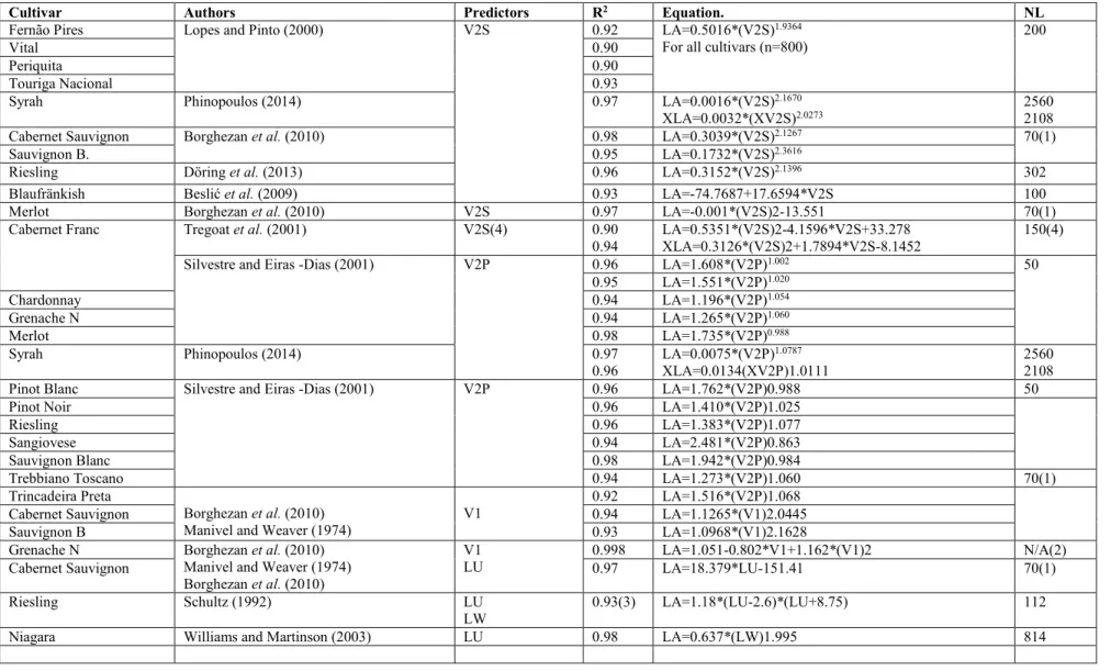
Table 1: Summary of studies regarding the prediction of the area of a single leaf, using Leaf

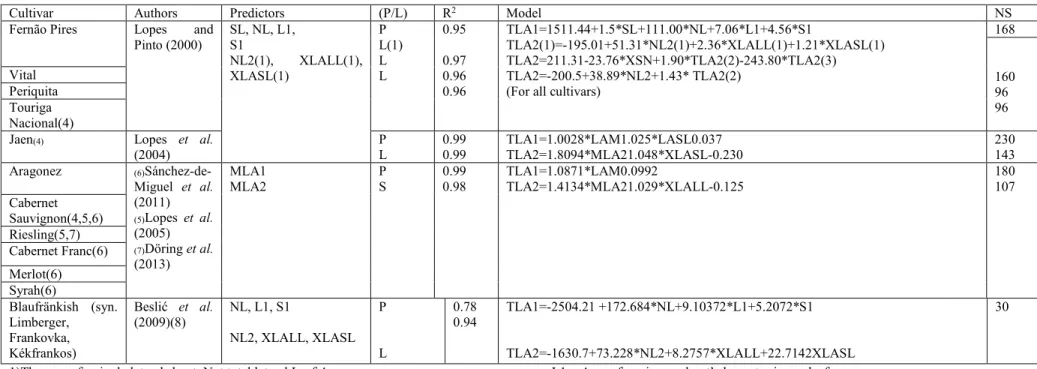
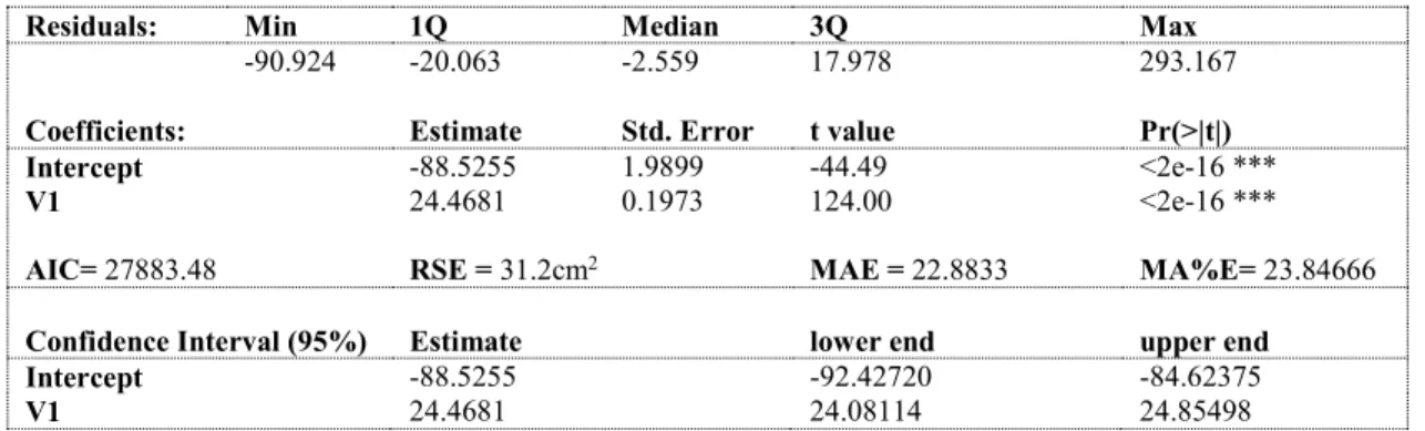
dimensions, adapted from Phinopoulos,(2014). ... 14 Table 2: Summary of studies regarding the prediction of the primary and lateral area of a single shoot (adapted from Phinopoulos, 2014) ... 18 Table 3: Correlation matrix between actual primary single leaf area (LA1) and the 5 variables: V1 = central vein length in cm; V2L = right lateral vein length in cm; V2R = left lateral vein length in cm; ML2S = sum of lateral veins of the primary leaf; n= 2964 leaves, cv. Trincadeira ... 30 Table 4: test statistics to equation 15: residuals, Akaike Information criterion (AIC), Residual Standard Error (RSE), Mean Absolute Error (MAE) and Mean Absolute Percent Error (MA%E) for linear

regression of Single primary leaf area (response variable) and central vein length (V1) in cm as predictor variable; Confidence Interval on 95% level for intercept and coefficient (V1); Signif. codes: 0 '***' 0.001 '**' 0.01 '*' 0.05 '.' 0.1 ' ' 1 ... 31 Table 5: test statistics to Equation 16, residuals, Akaike Information criterion (AIC), Mean Absolute Error (MAE) and Mean Absolute Percent Error (MA%E) for nonlinear regression of Single primary leaf area (EMLA, response variable) and central vein length (V1) in cm as predictor variable; Confidence Interval on 95% level for coefficients (a and b); (1) residuals of linear regression between fitted and observed values ... 33 Table 6: Akaike Information criterion (AIC), Residual Standard Error (RSE), Mean Absolute Error (MAE) and Mean Absolute Percent Error (MA%E) for nonlinear regression of Single primary leaf area (response variable) and sum of lateral vein lengths (log(V1)) in cm as predictor variable; Confidence Interval on 95% level for intercept and coefficient (log(V1)); Signif. codes: 0 '***' 0.001 '**' 0.01 '*' 0.05 '.' 0.1 ' ' 1 ... 35 Table 7: Akaike Information criterion (AIC), Residual Standard Error (RSE), Mean Absolute Error (MAE) and Mean Absolute Percent Error (MA%E) for linear regression of single primary leaf area (response variable) and sum of lateral vein lengths (ML2S) in cm as predictor variable; 95% level CI for intercept and coefficient (ML2S); Signif. codes: 0 '***' 0.001 '**' 0.01 '*' 0.05 '.' 0.1 ' ' 1 ... 36 Table 8: test statistics for equation 19; Akaike Information criterion (AIC), Mean Absolute Error (MAE) and Mean Absolute Percent Error (MA%E) for nonlinear regression of Single primary leaf area (EMLA, response variable) and sum of lateral vein lengths (ML2S) in cm as predictor variable; Confidence Interval on 95% level for coefficients (a and b); Signif. codes: 0 '***' 0.001 '**' 0.01 '*' 0.05 '.' 0.1 ' ' 1(1) residuals of linear regression between fitted and observed values ... 36 Table 9: test statistics for equation 21; Akaike Information criterion (AIC), Residual Standard Error (RSE), Mean Absolute Error (MAE) and Mean Absolute Percent Error (MA%E) for nonlinear regression of Single primary leaf area (response variable) and sum of lateral vein lengths (log(ML2S)) in cm as predictor variable; Confidence Interval on 95% level for intercept and coefficient (log(ML2S)) ... 38

(8)

VI

Table 10: Correlation matrix between actual lateral single leaf area (LA) and the 4 variables: V1 = central vein length ; V2L = right lateral vein length ; V2R = left lateral vein length ; LL2S = sum of lateral veins of the lateral leaf; n= 4072 leaves, cv. Trincadeira ... 38 Table 11: Akaike Information criterion (AIC), Mean Absolute Error (MAE) and Mean Absolute Percent Error (MA%E) for nonlinear regression of Single lateral leaf area (ELLA, response variable) and sum of lateral vein lengths (LL2S) as predictor variable; Confidence Interval on 95% level for coefficients (a and b) ... 41 Table 12: test statistics for equation29; Akaike Information criterion (AIC), Residual Standard Error (RSE), Mean Absolute Error (MAE) and Mean Absolute Percent Error (MA%E) for linear regression of Single lateral leaf area (response variable) and sum of lateral vein lengths (log(LL2S)) in cm as predictor variable; Confidence Interval on 95% level for intercept and coefficient (log(LL2S)) ... 42 Table 13: Results of the ANCOVA test, comparing a full model with the distinction of Primary and Lateral Leaves (Model 1) and a sub model without the interaction of Leaf Type (Model 2) ... 44 Table 14: Overview over all presented models for single primary leaf area (EMLA) estimation;

equation number (Eq. Nr.), Model equation, Predictor variable, adjusted R2_{, n= number of}

observations.; (1) adjusted R2_{for linear regressions between fitted values of nonlinear regression and}

original observations;(2) adjusted R2_{for linear regression of transformed variables; Type: p= primary}

single leaf, l= lateral single leaf ... 44 Table 15: between total primary shoot leaf area (TLA1) and the 5 variables: B1 = Biggest primary leaf area; ESL = effective shoot length; MLA1 = mean primary shoot leaf area; NL1 = Number of primary leaves; STA= Shoot area; n= 230 primary shoots, cv. Trincadeira ... 46 Table 16: test statistics for equation 34; Akaike Information criterion (AIC), Residual Standard Error (RSE), Mean Absolute Error (MAE) and Mean Absolute Percent Error (MA%E) for linear regression of Primary shoot Leaf Area (response variable) and Shoot Area (log(STA)) as predictor variable;

Confidence Interval on 95% level for intercept and coefficient (log(STA)) ... 48 Table 17: Results of the ANCOVA test, comparing a full model with the distinction of trimmed and untrimmed shoots (Model 2) and a sub model without the interaction of Treatment (Model 1)... 49 Table 18: test statistics for equation 39; Akaike Information criterion (AIC), Residual Standard Error (RSE), Mean Absolute Error (MAE) and Mean Absolute Percent Error (MA%E) for non-linear regression of Primary shoot Leaf Area (response variable) and Mean Primary Leaf Area (MLA1) as predictor variable; Confidence Interval on 95% level for coefficients a and b ... 52 Table 19: test statistics for equation 40; Akaike Information criterion (AIC), Residual Standard Error (RSE), Mean Absolute Error (MAE) and Mean Absolute Percent Error (MA%E) for non-linear regression of Primary shoot Leaf Area (response variable) and Mean Primary Leaf Area (MLA1) as predictor variable; Confidence Interval on 95% level for the Intercept and slope of log(MLA1) ... 53 Table 20: correlation matrix between total lateral leaf area (TLA2) and the 4 variables: B2 = biggest lateral leaf area; MLA2 = mean lateral shoot leaf area; NL2 = number of lateral leaves; S2= smallest lateral leaf; n= 149 primary shoots, cv. Trincadeira ... 54

(9)

VII

Table 21: test statistics for equation 41; Akaike Information criterion (AIC), Residual Standard Error (RSE), Mean Absolute Error (MAE) and Mean Absolute Percent Error (MA%E) for multiple linear regression of TLA2 (response variable) and Number of lateral leaves (NLL); Confidence Interval on 95% level for intercept and coefficients... 55 Table 22: test statistics for equation 42; Akaike Information criterion (AIC), Residual Standard Error (RSE), Mean Absolute Error (MAE) and Mean Absolute Percent Error (MA%E) for nonlinear regression of TLA2 and Number of lateral leaves (NLL); Confidence Interval on 95% level for coefficients a and b ... 56 Table 23: test statistics for equation 46; Akaike Information criterion (AIC), Residual Standard Error (RSE), Mean Absolute Error (MAE) and Mean Absolute Percent Error (MA%E) for nonlinear regression of TLA2 and Mean Lateral Leaf Area (MLA2) Confidence Interval on 95% level for Intercept and slope ... 58 Table 24: test statistics for equation 47; Akaike Information criterion (AIC), Residual Standard Error (RSE), Mean Absolute Error (MAE) and Mean Absolute Percent Error (MA%E) for nonlinear regression of TLA2 and Mean Lateral Leaf Area (MLA2) Confidence Interval on 95% level for Intercept and slope ... 58 Table 25: test statistics for equation 49; Akaike Information criterion (AIC), Residual Standard Error (RSE), Mean Absolute Error (MAE) and Mean Absolute Percent Error (MA%E) for nonlinear regression of TLA2 and Mean Lateral Leaf Area (MLA2) Confidence Interval on 95% level for Intercept and slope ... 59 Table 26: test statistics for equation 50; Akaike Information criterion (AIC), Residual Standard Error (RSE), Mean Absolute Error (MAE) and Mean Absolute Percent Error (MA%E) for nonlinear regression of TLA2 and Mean Lateral Leaf Area (MLA2) Confidence Interval on 95% level for Intercept and slope ... 60 Table 27: Overview over all presented models for Shoot Primary and Lateral Leaf Area (TLA1 and TLA2 respectively) estimation; equation number (Eq. Nr.), Model equation, Predictor variable, adjusted R2_{, n= number of observations.; (1) adjusted R}2_{for linear regressions between fitted values of}

nonlinear regression and original observations;(2) adjusted R2_{for linear regression of transformed}

variables; Type: p= primary shoot leaf area, l= lateral shoot leaf area leaf... 61 Table 28: test statistics for equation 23; Akaike Information criterion (AIC), Residual Standard Error (RSE), Mean Absolute Error (MAE) and Mean Absolute Percent Error (MA%E) for linear regression of Single lateral leaf area (response variable) and central vein length (V1) in cm as predictor variable; Confidence Interval on 95% level for intercept and coefficient (V1) ... 69 Table 29: test statistics to equation 24; Akaike Information criterion (AIC), Mean Absolute Error (MAE) and Mean Absolute Percent Error (MA%E) for nonlinear regression of Single primary leaf area (EMLA, response variable) and central vein length (V1) in cm as predictor variable; Confidence Interval on 95% level for coefficients (a and b); (1) residuals from linear regression of fitted values . 70

(10)

VIII

Table 30:test statistics to equation 25; Akaike Information criterion (AIC), Residual Standard Error (RSE), Mean Absolute Error (MAE) and Mean Absolute Percent Error (MA%E) for nonlinear regression of Single lateral leaf area (response variable) and central vein lengths (log(V1)) in cm as predictor variable; Confidence Interval on 95% level for intercept and coefficient (log(V1)) ... 70 Table 31: test statistics for equation 27; Residuals, Akaike Information criterion (AIC), Residual Standard Error (RSE), Mean Absolute Error (MAE) and Mean Absolute Percent Error (MA%E) for linear regression of Single lateral leaf area (response variable) and sum of lateral vein lengths (ML2S) in cm as predictor variable; Confidence Interval on 95% level for intercept and coefficient ( (LL2S) ... 71 Table 32: test statistics to equation 33; Akaike Information criterion (AIC), Residual Standard Error (RSE), Mean Absolute Error (MAE) and Mean Absolute Percent Error (MA%E) for linear regression of Shoot primary leaf area (response variable) and effective shoot length (ESL) as predictor variable; Confidence Interval on 95% level for intercept and coefficient (log(ESL)) ... 71 Table 33: test statistics for equation 34; Akaike Information criterion (AIC), Residual Standard Error (RSE), Mean Absolute Error (MAE) and Mean Absolute Percent Error (MA%E) for linear regression of Primary shoot Leaf Area (response variable) and Shoot Area (log(STA)) as predictor variable;

Confidence Interval on 95% level for intercept and coefficient (log(STA)) ... 71 Table 34: test statistics for equation 43; Akaike Information criterion (AIC), Residual Standard Error (RSE), Mean Absolute Error (MAE) and Mean Absolute Percent Error (MA%E) for linear regression of transformed lateral shoot leaf area (response variable) and Shoot Area (STA) as predictor variable; Confidence Interval on 95% level for intercept and coefficient (log(STA)) ... 72

(11)

IX

List of Abbreviations

B1 Area of biggest primary Leaf (estimated) B2 Area of biggest lateral Leaf (estimated)

BBCH Biologische Bundesanstalt für Land- und Forstwirtschaft, Bundessortenamt und CHemische Industrie

D_av. Average basal shoot diameter ELLA Estimation for single lateral leaf area EMLA Estimation for single primary leaf area

ESL Effective Shoot Length

L1 Area of the largest primary leaf of each shoot L2 Area of the largest lateral leaf of each shoot

LA Leaf Area

LA1 Area of single primary leaves

LA2 Area of single lateral leaves

LAI Leaf Area Index

LN Leaf order

LL2S Sum of lateral leaves’ lateral veins

M1 Mean of the largest and smallest primary leaf M2 Mean of the largest and smallest lateral leaf

MLA1 Mean primary Leaf Area (multiplied by Number of leaves) MLA2 Mean lateral Leaf Area (multiplied by Number of leaves) ML2S Sum of primary leaves’ lateral veins

NI Number of clusters per shoot

NL1 Number of primary leaves

NL2 Number of lateral leaves

r Pearson product-moment correlation coefficient S1 Area of the smallest primary leaf of each shoot S2 Area of smallest lateral leaf

SLT Shoot length to the apex

STA Shoot Area

TLA Total Leaf Area (primary and lateral) TLA1 Total primary leaf area per primary shoot TLA2 Total lateral leaf area per primary shoot

V1 Length of the central vein

V2L Length of the left lateral vein V2R Length of the right lateral vein

(12)

X

List of Equations

D_av. = (D1 + D2)/2 Equation 1 ... 23

STA = D_av * ESL Equation 2 ... 23

M1 = (B1 + S1)/2 Equation 3 ... 24 MLA1 = M1 * NL1 Equation 4 ... 24 M2 = (B2 + S2)/2 Equation 5 ... 24 MLA2 = M2 * NL2 Equation 6 ... 24 Y = a + b*x . Equation 7 ... 25 Y = a*xb_. _{Equation 8 ... 25}

ln(Y) = ln(a) + b*ln(x) Equation 9 ... 25

Y = exp( ln(a) + b * ln(x)) Equation 10 ... 25

MAE = (Σ | yi - ŷi |)/n Equation 11 ... 25

MA%E = 100 [Σ (| yi - ŷi |/ | yi |)]/n Equation 12 ... 25

EF = 1- Σ (yi -ŷ i)2_{/Σ (yi -ÿ)}2 _{Equation 13 ... 25}

Y = a + Ip*ap + (b + Ip*bp)*x Equation 14 ... 26

EMLA = -88.53 + 24.47*V1 Equation 15 ... 31 EMLA = 2.80671*V11.72443 _{Equation 16 ... 33} ln(EMLA) = 0.20499 + 2.06647*ln(V1) Equation 17 ... 34 EMLA = 1.227513*V12.06647 _{Equation 18 ... 34} EMLA = -118.16999 + 15.79790* ML2S Equation 19 ... 35 EMLA = 0.34159*ML2S2.11963 _{Equation 20 ... 36} ln(EMLA) = -1.384 + 2.223*ln(ML2S) Equation 21 ... 37 EMLA = 0.2505742*ML2S2.223 _{Equation 22 ... 37} ELLA = -49.6831 + 17.5523* V1 Equation 23 ... 39 ELLA = 1.47006*V11.99284 Equation 24 ... 39 ln(ELLA) = 0.23359 + 2.06359*ln(V1) Equation 25 ... 40 ELLA = 1.263127*V12.06359 _{Equation 26 ... 40} ELLA = -51.37653 + 9.98935 *LL2S Equation 27 ... 40 ELLA = 0.379622*LL2S2.072415 _{Equation 28 ... 41} ln(ELLA) = -0.985879 + 2.076138*ln(LL2S) Equation 29 ... 42 ELLA = 0.3731111* LL2S2.076138 _{Equation 30 ... 42} ELA = 0.3292296*V2S2.128 Equation 31 ... 43

ln(TLA1) = 3.09871 + 1.00825*ln(ESL) Equation 32 ... 47

TLA1 = 22.16933* ESL1.00825 _{Equation 33 ... 47}

ln(TLA1) = 4.28610 + 0.78548*ln(STA) Equation 34 ... 48

TLA1 = 72.68245* STA0.78548 _{Equation 35 ... 48}

(13)

XI

TLA1 = 1.087085 * MLA10.992 _{Equation 37 ... 50}

TLA1 = 18.24266 + 1.07309*MLA1 Equation 38 ... 51

TLA1 = 1.38195*MLA10.96797 _{Equation 39 ... 51}

ln(TLA1) = -0.03882 + 1.01515*ln(MLA1) Equation 40 ... 53

TLA1 = 0.9619238* MLA11.01515 _{Equation 41 ... 53}

Y = a* x + b*y + c*z + d Equation 42 ... 54

TLA2 = 7.4586*NL2 + 1.6889* NL22_{-0.01* NL2}3_{+ 51.254} _{Equation 43 ... 54}

TLA2 = 13.124*NL21.397 _{Equation 44 ... 55}

TLA2 = 0.02967056 * STA2.299 _{Equation 45 ... 56}

TLA2 = 23.60927 + 0.86053 *MLA2 Equation 46 ... 58

ln(TLA2) = 0.02688 + 0.97829 *MLA2 Equation 47 ... 58

TLA2 = 1.027245*MLA20.97829 _{Equation 48 ... 58}

TLA2 = 309.8331-5.0215*B2 + 0.9606*MLA2 Equation 49 ... 59

lnTLA2 = 0.81410-0.42244*B2 + 1.0875137 *MLA2 Equation 50 ... 60

(14)

XII

Abstract

Estimating a Vineyard’s leaf area is of great importance when evaluating the productive and quality potential of a vineyard and for characterizing the light and thermal microenvironments of grapevine plants. The aim of the present work was to validate the Lopes and Pinto method for determining vineyard leaf area in the vineyards of Lisbon’s wine growing region in Portugal, with the typical local red grape cultivar Trincadeira, and to improve prediction quality by providing cultivar specific models.The presented models are based on independent datasets of two consecutive years 2015 and 2016. Fruiting shoots were collected and analyzed during all phenological stages. Primary leaf area of shoots is estimated by models using a calculated variable obtained from the average of the largest and smallest primary leaf area multiplied by the number of primary leaves, as presented by Lopes and Pinto (2005). Lateral Leaf area additionally uses the area of the biggest lateral leaf as predictor. Models based on Shoot length and shoot diameter and number of lateral leaves were tested as less laborious alternatives. Although very fast and easy to assess, models based on shoot length and diameter were not able to predict variability of lateral leaf area sufficiently and were susceptible to canopy management. The Lopes and Pinto method is able to explain a very high proportion of variability, both in primary and lateral leaf area, independently of the phenological stage, as well as before and after trimming. They are inexpensive, universal, practical, non-destructive methods which do not require specialized staff or expensive equipment.

(15)

XIII

Resumo

A estimação da área foliar de uma vinha é de extrema importância quando se pretende avaliar o potencial produtivo e qualitativo da mesma, assim como para caracterizar a temperatura e radiação incidida no microclima da videira. O objetivo do presente trabalho é o de validar a metodologia Lopes e Pinto para determinar a área foliar de videiras em vinhas da região vitivinícola de Lisboa, em Portugal, para a casta Trincadeira. Desta forma melhorando a capacidade de previsão do modelo ao serem providenciados modelos específicos para a casta em estudo. Os modelos apresentados neste trabalho são baseados em dados independentes de dois anos consecutivos: 2015 e 2016. Durante todos os estados fenológicos foram recolhidos e analisados sarmentos com frutificações. A área foliar principal é estimada a partir de modelos que utilizam uma variável calculada a partir das médias da área foliar principal da maior e da menor folha da videira, multiplicada pelo número total de folhas principais, como descrito em Lopes e Pinto (2005). A área foliar das folhas netas utiliza ainda a área da maior folha neta como segundo preditor. Ao longo da dissertação foram também testados modelos baseados no comprimento e diâmetro do sarmento e número total de folhas netas, como metodologias alternativas com menores necessidades laborais. Apesar da facilidade e eficiência de análise, os modelos baseados no comprimento e diâmetro do sarmento não foram suficientemente capazes de prever a variabilidade da área foliar das folhas netas, suscetível à gestão da canópia. A metodologia descrita em Lopes e Pinto (2005) é capaz de explicar uma eleva proporção de variabilidade, quanto à área foliar primária e das folhas netas, independentemente do estado fenológico, assim como antes e depois da desponta. Esta metodologia é pouco dispendiosa, universal, prática, não-destrutiva, que não necessita de recursos especializados nem de equipamento dispendioso.

(16)

1

1 Introduction

1.1. Introduction

The plants leaf area (LA) is a parameter which is of significant importance, as it can provide viticulturists and researchers with important indications regarding the vineyard’s condition. Leaves are the organs where sun radiation is converted to carbohydrates through photosynthesis, thus LA is the total area which could intercept light, providing an indication of the plant’s photosynthetic capacity and transpiration.

As a measurable parameter, LA can be defined as the one sided area of the leaf surface, flattening it to expand its full surface, including any overlapping lobes. Leaf Area can then be estimated per single leaf, shoot, plant or per meter of canopy. In these cases, it refers to the total area of all leaves belonging to the said sets. Expressed as m2_{LA per m}2_{soil surface it gives the}

dimensionless Leaf Area Index (LAI), which is often used as parameter in viticulture to estimate the possible productivity regarding yield and quality of grapes, as it is well comparable between different training systems and row spacing.

Leaf Area is already widely used to estimate daily dry matter production in annual crops such as rice, wheat, maize, soy beans, sugar beet etc., as it is easy to obtain with indirect methods due to the herbaceous nature of these plants. In woody plants, such as trees and shrubs, and trellised crops such as the grapevine, the use of LA is limited for the moment. For example, the estimation of Leaf Area can be important for the calculation of Evapotranspiration for the implementation of energy balance models, and can be used to calculate irrigation quantities or to adapt volumetric irrigation to canopy characteristics. Difficulties to obtain these parameters are given due to the interference of the plant’s woody parts and / or the trellis system with total LA, when indirect methods by light extinction through the canopy are used.

It is understood that with its evident interest, grapevine Leaf Area could be more widely used, when easy, cost effective and precise estimation is possible.

(17)

2

1.2. Objectives

The aim of this work is to review the methods available for the estimation of grapevine Leaf Area and to adjust this methodology to the ampelography of the Portuguese variety Trincadeira. Providing a new and improved empirical model for the direct estimation of the area of a single leaf and the total Leaf Area of a shoot for this cultivar, based on the Lopes and Pinto (2005) methodology. This will allow LA to be used more widely in viticulture and research, as it will be obtainable without the use of special equipment, using nothing but instruments which measure length and an equation provided by the authors.

The importance of LA and the benefits from an easy method for its estimation are described below.

(18)

3

2 Literature Overview

2.1. Importance of Leaf Area

Leaf Area is typically defined as the one sided area of a leaf lamina. As such it can be calculated per single leaf (Carbonneau 1976 a; Lopes and Pinto 2000), a single shoot, divided into primary and lateral leaf area (Carbonneau,1976 b; Barbagallo et al., 1996; Lopes and Pinto, 2005), but also for the whole plant or per square meter ground (Watson, 1947) and consequently for the entire vineyard.

The fruiting capacity of grapevines in a given climatic region is largely determined by their total Leaf Area, and the proportion of shaded Leaf Area, provided that other factors are not restrictive (Kliewer and Dokoozlian, 2005). Excessive Leaf Area can indicate high vigor (Champagnol, 1984), while an insufficient Leaf Area may impair the vineyard’s productive capability. According to Kliewer and Dokoozlian (2005), there must be an equilibrium between Leaf Area and yield, to achieve the desirable fruit ripeness and thus, wine quality, rendering Leaf Area a basic indicator to determine vine balance. In the same study, they provide the ideal Leaf Area to crop ratios for several cultivars.

Leaf Area can also be used to adjust the amount of dosage of plant protection products, to avoid under dosage which would provide insufficient protection against pests, or over dosage, which has adverse environmental effects and increases costs (Siegfried et al., 2006).

It has been established (Bravdo et al., 1984; Hepner et al., 1985), that Crop Load (Ravaz Index), is also strongly correlated to wine quality. Crop Load is calculated as the ratio of yield of grapes, to the pruning weight of the following winter (Ravaz, 1903). However, Cohen et al., (2000), suggest that the Leaf Area, rather than pruning weight, should be utilized for the expression of Crop Load, given that photosynthesis and other metabolic processes in the leaf are responsible for changes in fruit quality, rather than pruning weight per se. The reinvention of Crop Load based on Leaf Area rather than pruning weight can provide a more easily applicable and representative parameter, as it will better reflect the growing conditions of the current, rather than the previous season (Cohen et al., 2000).

2.2. Other parameters related to Leaf Area

2.2.1. Leaf Area Index

The Leaf Area Index (LAI) is a dimensionless quantity defined as the ratio between the estimated area of vine foliage and the vineyard’s soil, both expressed in m2_{(Champagnol, 1984;}

(19)

4

Apart from providing an indication of the photosynthetic surface, LAI is also a fundamental indicator for the understanding of the plant’s responses to environmental factors (Lopes et al., 2004) and its quantification allows the evaluation of cultural practices, especially those related to leaf management and the training system (Smart, 1995).

Knowledge of the vineyard’s LAI can lead to conclusions regarding water balance (Beslić et al., 2009), the competition with weeds (Guisard et al., 2010), whole-plant assimilation, light interception and bunch exposure (Döring et al., 2013). As these factors affect the plant’s microclimate, conditions of moisture and temperature related to disease pressure and fruit quality and quantity (Smart, 1985; Sánchez-de-Miguel et al., 2011), can also be predicted. Changes in LAI could also give indications as to the extent of phytosanitary damages (Borghezan et al., 2010). Based on the LAI, several other parameters can be calculated, such as the Leaf Area per yield ratio, the ratio of exposed Leaf Area per total Leaf Area etc., ratios that are very important for viticultural decision making (Smart and Robinson, 1991), and influencing fruit quality (Petrie et al., 2000 a,b). For example, the estimation of Leaf Area Index can be important for the calculation of Evapotranspiration for the implementation of energy balance models, and can be used to calculate irrigation quantities (Fuchs et al., 1987) and to adapt volumetric irrigation to canopy characteristics (Guisard et al., 2010).

2.2.2. Exposed leaf area

Another useful parameter is exposed leaf area (ELA), which is the Leaf Area of the external leaves, which are exposed to sunlight. This parameter is very important, given the fact that 90% of photosynthesis is carried out by these leaves and, thus, the overall productivity of the vineyard (Smart 1973, Schneider 1992, Sánchez-de-Miguel et al. 2010, Baeza et al., 2010). It is estimated that around 0.9-1.5 m2 of ELA are necessary for the ripening of 1kg of grapes (Carbonneau, 1989; Kliewer and Dokoozlian, 2005).

An estimation of the ELA for a given plot can be used before planting a vineyard, to set the desired performance targets per meter of row or hectare. In designing the plantation, ELA estimation will allow the calculation of row spacing and canopy height (Sánchez-de-Miguel et al. 2010).

(20)

5

2.3. The evolution of Leaf Area during the growing season

2.3.1. Phyllotaxy

The leaf of the grapevine consists of the petiole (stalk) and the lamina (blade). Trincadeira and most grapevine leaves have 5 lobes and 5 main veins arising from a single point at the junction of the petiole to the lamina (Iland et al., 2011). In grapevines that are not juvenile, the phyllotaxy is distichous. This means that the leaves are produced alternating on the opposite sides of the stem, so that the shoot is bilaterally symmetrical with respect to leaf formation and the angle between successive leaves is 180°. In contrary, in juvenile grapevines, phyllotaxy is spiral and the angle between leaves is 145° (Iland et al., 2011). This juvenile stage ends, when 6-10 leaves have developed (Mullins, et.a., 1992)

2.3.2. Fixed and Free Growth

After budburst, shoots sprout from buds formed during the previous season, containing preformed nodes, inter-nodes and inflorescence primordia. Nodes formed in a latent bud before it goes into dormancy, are called ‘fixed’ nodes. There are 6 to 10 fixed nodes (Iland et al., 2011), or 6 – 12 (Champagnol, 1984; Sánchez-de-Miguel et al., 2010), in a N+2 bud and this implies that the structures found on the first 6 – 10 nodes that occur in a season, including the expanded leaves, are a result of the fixed growth of nodes that were preformed in the bud during the previous year. Fixed growth is a result of cell enlargement of preformed primordial cells and not of the formation of new cells (Sánchez-de-Miguel et al., 2010). Leaf and inflorescence primordia can be seen at the shoot tip from the time the shoot emerges from a bud (Iland et al., 2011).

On the other hand, nodes of higher ranks, or free nodes, are the result of free growth of the apical meristem which requires cell division, thus the formation of new cells. Free growth is the result of the elongation and production of new primordia in the apical meristem activity (Sánchez-de-Miguel et al., 2010). The apical meristem has two functions: the production of new organs and new tissue. Growth occurs at the tip of the shoot and cell division mainly occurs in the apical meristems (Iland et al., 2011). During the season, shoot growth is a combination between fixed growth and free growth (Phinopoulos, 2014).

2.3.3. Shoot growth and leaf growth

The formation of new nodes at the apex usually stops around flowering (Iland et al., 2011). At this point, there may be up to 30 – 35 nodes. The elongation of a single node may last from 7 to

(21)

6

40 days and internode length may vary from 1 to 25 cm (Iland et al., 2011). According to Champagnol (1984), elongation in both nodes and leaves can last between 15-25 days, while radial expansion may be unlimited in time but is interrupted at the end of each period of growth. While the node reaches its final length after about 25 days, and does not increase further, its width or diameter may continue increasing under favorable conditions (Champagnol 1984). Young leaves grow for 3 to 5 weeks (Huglin and Schneider, 1998), or until they reach their final dimensions. Leaf development is divided into two phases: a rapid growth phase of about 250 degree days, followed by a plateau in Leaf Area (Wermelinger and Koblet, 1990). Most primary leaves usually grow to reach a similar Leaf Area, while lateral leaves usually do not reach the same size, although they can surpass primary leaves in number (Wermelinger and Koblet, 1990). According to the same authors, the leaves remain in a productive condition for about 650 degree days after they reach their full size. At the age of 900 degree days the leaves become senescent, which is indicated by a sudden decrease of nitrogen and water content.

2.3.4. Lateral shoots

Lateral shoots or summer laterals (order N+1), are shoots that arise from the first bud of the axil of the leaves of a current season shoot. These are prompt buds, in the sense that they start growing the same year when they are formed. The growth of lateral shoots can be strongly stimulated by the removal of the shoot tip by trimming, with the maximal effect occurring when at least 9 nodes are removed (Iland et al., 2011). It seems that the dormancy is caused not only by the continuous development of buds on the primary shoots, but also by young leaves (Champagnol, 1984). Lateral shoots may continue growing even when the growth of the primary shoot has stopped. A greater number and length of lateral shoots is associated to high vigor, well exposed primary shoots and severe pruning (Iland et al., 2011).

Lateral Leaf Area can provide an additional source of leaves for photosynthesis. This is useful when a part of the primary Leaf Area has been lost due to operations such as wire lifting, pests and diseases, abiotic stress (water and heat), or due to other reasons such as hail or frost. Lateral shoots are considered beneficial when they are located on the upper part of the shoot and can intercept sufficient sunlight for photosynthesis and in lower parts of the shoots where they may protect the bunches from intense sunlight. However, extensive lateral shoot growth is considered undesirable, as it is a sign of high vigor, vine growth imbalance and may cause an disadvantageous microclimate and shading, especially in the bunch zone (Smart, 1985).

In general, lateral leaves represent younger tissue, as they emerge at a later stage. While they initially consume resources produced by mature leaves, they later start offering a greater contribution to total photosynthesis. Hale and Weaver (1962), consider that lateral shoots

(22)

7

become sources of photosynthetic products after developing two or more fully expanded leaves. In general, the quantity and the proportion of lateral Leaf Area can vary according to the variety, the growing conditions and the cultural practices, but it usually represents an important part of the total Leaf Area. Lateral Leaf Area can comprise 6 -40% (Iland et al., 2011), or 22 – 44% (Paliotti et al., 2000) of total Leaf Area and may have, in some cases, an important contribution to fruit ripening. Poni et al. (2006) point out that, after defoliation of six primary leaves, lateral shoots can contribute to compensate leaf area loss and lead to improved berry composition. Lateral Leaf Area can also represent an even higher proportion of the total Leaf Area under conditions of high vigor (Huglin and Schneider, 1998). In fact, lateral Leaf Area can be a precise indicator of vigor, as vigorous shoots are characterized by a great development of lateral shoots and a large lateral per total Leaf Area ratio. The possibility to distinguish between primary and lateral Leaf Area is also important for assessing the viticultural potential of the training system and the terroir (Ollat et al., 2001).

2.3.5. Rate of leaf emergence

The rate of leaf appearance presents a symmetric pattern in time. It progressively increases during the first weeks and then decreases to zero during the ripening period. If there are no drought conditions, this is done by endogenous stimuli (Palchetti et al., 1995). The speed of leaf appearance and development is strongly related to temperature, for both exposed and shaded leaves. In fact, leaves develop at the same speed, regardless of the canopy zone where they belong, thus leaf development speed is not affected by light. The time required for a leaf to grow, increases along the growing season (Schultz, 1993). Other factors such as pruning severity, growth direction, crop load, light exposure and nutrient availability, may also affect leaf appearance to some extent. Leaf emergence is not affected by the training system, but shoots growing vertically present a much higher vigor than those growing downwards (Palchetti et al., 1995). Shoot growth and leaf appearance rate is highly impacted by soil water deficit, which can contribute to explain the decline in shoot and leaf growth in hot and dry regions, towards end of summer (Lebon et al., 2006) Shoot growth rates seem to be proportional to leaf growth rates, at least until before leaf fall (Wermelinger and Koblet, 1990). In fact, the shoot’s growth model is very similar to that of the leaves, because the grapevine is a deciduous plant (Sánchez-de-Miguel et al., 2010).

(23)

8

2.3.6. Shoot and Leaf Area growth

The pattern of the vine’s canopy development is similar to that of its shoots (Mullins et al., 1992). Environmental factors also affect shoot growth. In areas with lack of water, shoot growth may cease earlier. If there are no restrictive environmental factors the stop of shoot growth is caused by endogenous factors, that is, the alteration of hormonal balance within the plant. As shoot growth proceeds, the ratio of the number of older leaves to that of younger leaves increases. Shoot growth slows down or stops. The organogenic activity of the apex stops and the apex dries and falls off. The proportion of adult leaves that have ceased to grow, to young leaves can be a factor predicting the oncoming cease of shoot growth. This can occur on both short and very long shoots, with small or large leaves (Champagnol, 1984).

The bunches become the most important sinks of photosynthesis products after flowering, but shoots and Leaf Area continue to increase due to the increase in structural components. However, lateral shoots may continue growing even when primary shoot growth has slowed or ceased, especially in conditions of high vigor (Iland et al., 2011).

Shoot growth is slow after budburst but it later becomes exponential, reaching the highest rates around flowering, after which shoot growth rate decreases. In field conditions, the curve becomes sigmoidal (Iland et al., 2011; Mullins et al., 1992). The exponential growth cannot persist in a complex organism such as the grapevine, due to increasing competition for carbohydrates from other organs, which cause a cessation of cell division and enlargement (Mullins et al., 1992).

2.3.7. Factors affecting shoot growth

Shoot growth can be affected by water and nutrient supply, as well as by climatic factors. Water deficit can result in reduced vigor and reduction in Shoot Length and Leaf Area, having a greater effect on lateral Leaf Area (Iland et al., 2011). It seems that node elongation is sensitive to water stress, while the formation of new nodes is not affected to the same extent.

The rate of shoot growth increases with the increase of air and soil temperature. Cool to moderate temperatures favor internode elongation and vigor, while high temperatures favor node production. Lack of light results in longer internodes and exposure to wind may reduce shoot growth.

As far as cultural practices are concerned, high plantation density decreases shoot growth but may leave the Leaf Area per area of soil (LAI) unaffected. Vines with a minimal pruning have a higher Leaf Area than cane pruned vines. Shoot thinning can stimulate the growth of the

(24)

9

remaining shoots. Shoot positioning also affects shoot growth, with vertically positioned shoots being more vigorous. (Iland et al., 2011)

The variations in shoot growth also affect the leaves but the fluctuations in light intensity affect leaves to a greater extent. Leaves that grow in shaded conditions are usually thinner and abscise earlier than those exposed to sunlight. This may also be due to the leave’s movement, seeking light. Leaves in vines with lack of water usually have smaller epidermal cells and a lower nitrogen concentration. In this case, leaves are smaller and present a more leathery texture (Iland et al., 2011).

2.4. Estimation of Leaf Area

It is understood from all the above, that a rapid, easy and cheap method to estimate Leaf Area could be of significant use to growers. There are several methods of determining LA, which can be categorized as direct or indirect. Mabrouk and Carbonneau (1996), define as direct methods those where the measurements are done directly on plant organs whereas indirect methods are those where Leaf Area is estimated from the measurements of light. It is possible to further subdivide these methods in destructive or non-destructive, depending on if their application will destroy or maintain the measured leaf area respectively.

2.4.1. Indirect methods

Indirect methods do not measure Leaf Area per se, but use equipment to measure other parameters, from which the LAI can be estimated, such as the measurement of light extinction through the canopy (Grantz and Williams, 1993; Sommer and Lang, 1994; Oliveira and Santos, 1995; Ollat et al., 1998; Patakas and Noitsakis, 1999, Cohen at al., 2000). These methods only seem to be valid after the canopy reaches a certain size and the measurements have to be done below a clear sky and a sun declination that precludes the overlapping of shadows (Oliveira and Santos, 1995). Furthermore, the accuracy of Gap fraction Inversion seems to vary according to the variety and does not give accurate estimates for most varieties (Cohen et al., 2000). In other empirical models, Leaf Area is calculated using temperature summation (Schultz, 1992; Bindi et al., 1997), or remote canopy imaging (Dobrowski et al., 2002). These methods are rapid and relatively easy to implement but they have the significant drawback that they require expensive special equipment, which is beyond the budget of most growers.

Grantz and Williams (1993) found the results, obtained with the conventional protocol of the LAI-2000 Plant Analyzer, insufficient and consistently underestimating Leaf Area. Sommer and Lang (1994) compared two devices (LAI-2000 and Demon device) that measure natural light

(25)

10

that can pass through the canopy and have special filters which reduce the effect of scattered light on measurements. They found the results provided by DEMON satisfactory, while the LAI-2000 systematically underestimated Leaf Area. Ollat et al. (1998) also tested the LAI-2000 Plant Canopy Analyzer, on Bordeaux vineyards. They found that results for single vines were not satisfactory and that good relationships could only be obtained if five or more consecutive vines were used. Regardless of the protocol used, the device underestimated the Leaf Area of small vines and overestimated that of large vines. In general, the performance of the LAI-2000 was considered mediocre, in accordance with Grantz and Williams (1993) and Sommer and Lang (1994). Furthermore, Tregoat et al. (2001), point out that the LAI-2000 is a very expensive device.

2.4.2 Most Recent Development of indirect methods

Newer methods work in a similar way, but use a light source that is part of the equipment, rather than ambient light. One such method of indirect determination of Leaf Area is the Normalized Difference Vegetation Index (NDVI). Drissi et al. (2009) tested the GreenSeeker RT100 system on VSP Merlot. This is a portable device, using high intensity light emitting diodes (LED) that measures the light reflected by the canopy. The system seems to be unaffected by background light and temperature. Although the device is usually used to make vertical measurements, the authors used it to measure the canopy horizontally, with a screen placed behind it. It is understood that this complicates the procedure and also limits its applicability to VSP systems. One advantage of the equipment is that is can be connected to GPS systems and yield Leaf Area maps of the vineyard. As far as airborne NDVI is concerned, a recent study by Hall et al. (2009), concluded that it was effective in mapping spatial variability in planimetric canopy area, thus contradicting previous studies which claimed that Leaf Area could be predicted by airborne NDVI and attributed this correlation to a proxy relationship between NDVI and canopy area, which could then be a predictor of Leaf Area. They also point out, that the relationship depends on the density and the extent of Leaf Area.

Arnó et al. (2012) used ground based light detection and ranging sensors (LiDAR), to estimate grapevine Leaf Area. This system measures the time a laser pulse needs to return, after it has been reflected by the canopy and the angle of the beam to the leaf. Although this system provides a relatively good estimation of Leaf Area, the processing of the data is very complicated. The accuracy of the method varies with the number of scans and several measurements have to be performed to obtain sufficient accuracy. Furthermore, the Leaf Area is given for length of canopy and not per vine or field area. Furthermore, the results seemed to be

(26)

11

different if made from the other side of the canopy, a fact which indicates its lack of accuracy (Arno et al., 2012)

There have been some attempts to develop methods of Leaf Area estimation that do not require sophisticated equipment. Ollat et al. (2001), obtained disappointing results with the use of pictures taken with a commercial digital camera. In a similar approach, Espinosa et al. (2010), used a commercial digital camera to estimate Leaf Area, and analyzed the images with computer software. This method however, required pictures to be taken from a specific distance, using a white fiberglass background. The background diminishes the effect of sky brightness on the measurements, but makes measurements less practical. Furthermore, it has only been tested for single, vertical trellises, with limited applicability to other training systems.

A more recent attempt to eliminate the use of complex and expensive devices has been done by Fuentes et al. (2012). They developed an application (Viticanopy®) which can be installed on smartphones and Tablets and can use the camera and GPS features of these devices to estimate Leaf Area. Upwards facing pictures from beneath the canopy are transformed, using thresholds to obtain canopy architectural parameters for grape vines i.e. LAI, Canopy cover, Crown Porosity and Clumping Index, using automated analysis by applying gap size assessment algorithms (Macfarlane et al., 2007; Fuentes et al., 2008; Fuentes et al., 2014).

Recently the app has been validated against different reference methods as Licor LAI-2000 and MatLab and has shown high correlations of R2_{= 0.96 and R2 = 0.97 respectively (De Bei et. al.,}

2016). Although this kind of software might solve the problem of expensive equipment, it still maintains most the disadvantages of the older imaging methods to estimate Leaf Area.

In general, the disadvantages of the imaging methods include, that most devices require frequent calibration and specific sampling protocols (Ollat et al., 1998) a fact that implies that they should be operated by specialized staff. It has also been demonstrated (Grantz and Williams, 1993; Sommer and Lang, 1994; Cohen et al., 2000), that under vigorous conditions or dense canopies these methods often underestimate Leaf Area, as leaves are overlapping. The remote-sensing approach seems to have several limitations, such as leaf clumping (Cohen et al., 2000; Blom and Tarara, 2007; López-Lozano and Casterad, 2013) and the variation in color of the vegetative material within the canopy. It is sometimes difficult to distinguish the Leaf Area of a single plant within a row, as the canopies of neighboring plants are often overlapping (Blom and Tarara, 2007). It must also be pointed out, that the results always include non-leafy elements (Cohen et al., 2000), thus do not reflect Leaf Area alone. In fact, a recent study by López-Lozano and Casterad (2013), demonstrated that not only the sampling protocol, but also the position of the sun during the measurements, strongly influence the results for Leaf Area estimation. The same authors point out, that most optical devices for indirect measurement of

(27)

12

Leaf Area Index (LAI) from canopy-transmitted light are tailored for homogeneous canopies, thus limiting their application to discontinuous canopies such as vertically trained vineyards. In order to obtain non-biased LAI estimates, the homogeneity of the canopy fraction measured along the ceptometer at each individual reading is a major requirement (López-Lozano and Casterad, 2013). In fact, most devices for Leaf Area estimation are designed with a mathematical model assumption that individual leaves are randomly and uniformly distributed. Row crops and trellised vineyards in particular, generally violate these assumptions and for this reason, large systematic errors in Leaf Area estimation can arise (Lang et al., 1985).

Another disadvantage of the above mentioned methods is that they treat Leaf Area as a whole, without distinguishing between primary and lateral leaves (Smart and Robinson, 1991; Lopes and Pinto, 2005). Distinguishing the two Leaf Areas and estimating them separately is important, as their physiological activity is different (Sánchez-de-Miguel et al., 2011).

2.4.3 Direct methods

Contrary to indirect methods, direct methods consist of direct measurements of samples of leaves and shoots. They are considered more accurate but also more laborious (Mabrouk and Carbonneau, 1996). They can be categorized as destructive and non-destructive.

2.4.4 Destructive methods

Destructive methods require the removal of leaves and transporting them to a laboratory. Leaf Area can then be determined by special Leaf Area measuring devices, by planimeters, or by determining the area to weight ratio (Sepúlveda and Kliewer, 1983). The relation between blade dry or fresh weight and Leaf Area has also been confirmed by Tregoat et al. (2001), although it seems that ageing leaves become heavier relative to their size (Wermelinger and Koblet, 1990). Although leaf fresh weight was found to have a relatively good relation to Leaf Area and does not require special equipment (Sepúlveda and Kliewer, 1983), its applicability seems to be limited, as it is a destructive method. These methods are considered being easy to implement and produce accurate results (Sommer and Lang, 1994), but most of them also require some sort of equipment. Apart from being laborious, time-consuming and reducing the plant’s photosynthetic Leaf Area (Lopes and Pinto, 2005), they also present the disadvantage that the evolution the Leaf Area of a specific plant or shoot cannot be monitored along the growing season, as the leaves are destroyed (Lopes et al., 2004).

(28)

13

2.4.5 Non-destructive methods

Non-destructive direct methods require portable versions of the equipment described above, which could be transported to the field and perform the measurements there. These are even more expensive and difficult to use on the field (Lopes and Pinto, 2005). Another possibility of a non-destructive and direct method to determine Leaf Area is to exploit the empirical relationship found between easily measurable parameters of leaf blades or shoots, and Leaf Area.

2.4.5.1 Estimation of single Leaf Area

There are several statistical models that can estimate the area of a single leaf with relatively good accuracy. Carbonneau (1976 a) found a good relation between the sum of the length of the two lateral veins and the total area of a single leaf. He pointed out, that by measuring the two lateral veins, the non-symmetric effect usual to grapevine leaves is eliminated and that they are usually correlated to either the length, or the width of the leaf. After the study mentioned above, several authors have suggested models for the determination of the area of a single leaf, using empirical models. Many models use the length of primary or lateral veins, while others use maximum leaf length and width. A summary of these studies and the models obtained, is presented in table 1.

Silvestre and Eiras-Dias (2001), also found a good relation between the area of a leaf and the distance from the central vein to the end of the right lateral vein, but they point out that this is a predictor which is difficult to measure. They rejected the use of the central vein, giving a correlation lower than 95%. Manivel and Weaver (1974), found good relations between Leaf Area and the length of the petiole.

(29)

14

Table 1: Summary of studies regarding the prediction of the area of a single leaf, using Leaf dimensions, adapted from Phinopoulos,(2014).

Cultivar Authors Predictors R2 _Equation. _NL

Fernão Pires Lopes and Pinto (2000) V2S 0.92 LA=0.5016*(V2S)1.9364

For all cultivars (n=800)

200

Vital 0.90

Periquita 0.90

Touriga Nacional 0.93

Syrah Phinopoulos (2014) 0.97 LA=0.0016*(V2S)2.1670

XLA=0.0032*(XV2S)2.0273 2560 ₂₁₀₈

Cabernet Sauvignon Borghezan et al. (2010) 0.98 LA=0.3039*(V2S)2.1267 ₇₀₍₁₎

Sauvignon B. 0.95 LA=0.1732*(V2S)2.3616

Riesling Döring et al. (2013) 0.96 LA=0.3152*(V2S)2.1396 ₃₀₂

Blaufränkish Beslić et al. (2009) 0.93 LA=-74.7687+17.6594*V2S 100

Merlot Borghezan et al. (2010) V2S 0.97 LA=-0.001*(V2S)2-13.551 70(1)

Cabernet Franc Tregoat et al. (2001) V2S(4) 0.90

0.94 LA=0.5351*(V2S)2-4.1596*V2S+33.278 XLA=0.3126*(V2S)2+1.7894*V2S-8.1452 150(4)

Silvestre and Eiras -Dias (2001) V2P 0.96 LA=1.608*(V2P)1.002 ₅₀

0.95 LA=1.551*(V2P)1.020 Chardonnay 0.94 LA=1.196*(V2P)1.054 Grenache N 0.94 LA=1.265*(V2P)1.060 Merlot 0.98 LA=1.735*(V2P)0.988 Syrah Phinopoulos (2014) 0.97 0.96 LA=0.0075*(V2P)1.0787 XLA=0.0134(XV2P)1.0111 2560 2108

Pinot Blanc Silvestre and Eiras -Dias (2001) V2P 0.96 LA=1.762*(V2P)0.988 50

Pinot Noir 0.96 LA=1.410*(V2P)1.025

Riesling 0.96 LA=1.383*(V2P)1.077

Sangiovese 0.94 LA=2.481*(V2P)0.863

Sauvignon Blanc 0.98 LA=1.942*(V2P)0.984

Trebbiano Toscano 0.94 LA=1.273*(V2P)1.060 70(1)

Trincadeira Preta

Borghezan et al. (2010) Manivel and Weaver (1974)

V1 0.92 LA=1.516*(V2P)1.068

Cabernet Sauvignon 0.94 LA=1.1265*(V1)2.0445

Sauvignon B 0.93 LA=1.0968*(V1)2.1628

Grenache N Borghezan et al. (2010)

Manivel and Weaver (1974) Borghezan et al. (2010)

V1

LU 0.998 LA=1.051-0.802*V1+1.162*(V1)2 N/A(2)

Cabernet Sauvignon 0.97 LA=18.379*LU-151.41 70(1)

Riesling Schultz (1992) LU

LW 0.93(3) LA=1.18*(LU-2.6)*(LU+8.75) 112

(30)

15

1)It is not clear whether the sample contained 70 leaves in total, or per cultivar 2)Sample size of 10 shoots at veraison.

3)Equation was calibrated using equations with R-squared values from 0.93 to 0.97 4)Separate models for Primary and Lateral Leaves. Number of primary and lateral leaves not specified

LA = Leaf Area of Primary Leaves

LL = Maximum leaf lamina length usually from tip to lowest point but not to petiolar sinus

LU = Leaf length where the exact method of determination is not exactly specified LW = Largest leaf lamina width, perpendicular to central vein

V1 = Length of central vein, or leaf lamina length from petiolar sinus to tip V2P = Product of the lengths of the two lateral veins

V2S = Sum of the lengths of the two lateral veins XLA = Leaf Area of Lateral Leaves

Cultivar Authors Predictors R2 _Equation. _NL

De Chaunac Williams and Martinson (2003) LW 0.96 LA=0.672*(LW)1.963 995

Cabernet Sauvignon Tsialtas et al. (2008) 0.87 LA=19.385*LW-144.59 18

Grenache N Manivel and Weaver (1974) 0.998 LA=1.051-0.109*LW+0.469*(LW)2 N/A(2)

Cencibel Montero et al. (2000) 0.968 LA=0.647*(LL)1.956 1739

Chenin blanc Sepúlveda and Kliewer (1983) LL 0.975 LA=2.49+0.68*(LL*LW) N/A

Chardonnay LL*LW 0.969 LA=3.17+0.69(LL*LW)

Gutierrez and Lavin (2000) 0.93 LA=2.0857+0.6257(LL*LW)

Cencibel Montero et al. (2000) 0.987 LA=0.587*(LL*LW) 1739

Concord Elsner and Jubb (1988) LW*V1

(LW)2+(V1)2 0.984 0.988 LA=-3.01+0.85*(LW*V1) LA=-1.41+0.527*(LW)2_+0.254*(V1)2 500

Asgari Eftekhari et al. (2011)

V1+LW V1*LW 0.920 0.926 LA=0.142*(V1+LW)2+0.796*(V1+LW) LA=-0.001*(V1*LW)2+0.860(V1*LW)+0.845 1251 1247 Keshmeshi Shahroodi Khalili

(31)

16

Montero et al. (2000) found that the use of maximum width, leaf length and petiole length were not as closely associated to Leaf Area as the combination of leaf width and leaf length, although they also obtained high determination coefficients. Sepúlveda and Kliewer (1983), consider that the use of maximum leaf length and width as single predictors also have high correlation coefficients, but smaller than the combination of both and they have a bigger standard error and highly negative intercepts. For these reasons, they do not consider them as good estimators of Leaf Area. Smith and Kliewer (1984) found the product of maximal leaf length and maximal leaf width to be the best predictors for the Leaf Area of Thompson Seedless (syn. Sultana), but rather than providing a single model, they presented different equations for bloom, veraison and bloom of the following year. Williams and Martinson (2003) also found a good correlation between central vein length, the square of central vein length, the product of central vein length, leaf width and Leaf Area, but they obtained the best results with leaf width, as it uses only one predictor and had a better accuracy. Eftekhari et al. (2011) also found central vein length and leaf width to be good predictors (R-squared =0.917, R-squared =0.881 respectively) but results with the combination of both were better. It seems that in studies with a larger sample size, more predictors have good results.

Studies conducted by Guisard and Birch (2005) and more recently Guisard et al. (2010), compared several of these methods, concluding that the most important variables for the estimation of the area of a single leaf are the length and the width of the leaf, with the lengths of veins usually improving the accuracy of the models. Borghezan et al (2010) maintain that the models should be adapted to each variety separately.

These methods are very simple and accurate and the area of a single leaf can be rapidly calculated without the use of any special equipment. It is usually easier to find and measure the central vein and/or the maximum width of a leaf, than to measure the lateral veins. Furthermore, the models based on the measurement of the main vein only, present the extra advantage of requiring a single measurement to determine Leaf Area, as opposed to the measurement of lateral veins, which always requires the length of both lateral veins. However, a general conclusion that can be reached from the results of previous works, as described in table 1, is that the use of two predictors for the determination of the area of a single leaf always provides more accurate estimates. In this sense, the use of the two veins, or the combination of the length of the lateral veins and the length of the central vein, usually provide better accuracy than the use of the central vein only. Given that the dependent variable (leaf area) is a two dimensional variable, it is also logical to assume that the product of two linear (one dimensional) measurements would provide better results, than one single linear measurement. Furthermore, measuring two parameters on a leaf (such as the two lateral veins) accounts for anomalies,