Economic value added assessment applied to the portuguese SME during the crisis period

Texto

(1)ECONOMIC VALUE ADDED ASSESSMENT APPLIED TO THE PORTUGUESE SME DURING THE CRISIS PERIOD. Catarina Gonçalves de Oliveira. Dissertation submitted as partial requirement for the conferral of Master in Accounting. Supervisor: Prof. Doutor Pedro Leite Inácio, Assistant Professor, ISCTE Business School Finance Department. April, 2014.

(2) Abstract Performance measurement has, over the past two decades, been a popular topic amongst academic and professional practitioners. Using a database containing the financial statements of the biggest and best 315 Portuguese SME, we assessed the economic value added by those companies for the triennium of 2008-2010. The findings indicate that globally, for the period of 2008-2010, the companies have not created value for their shareholders. Nevertheless, “Electrical Equipment” and “Commercial Services and Supplies” were the only two sectors that contributed, with a positive MVA, to this globally negative scenario. These findings may be useful for financial managers, investors and corporate finance consultants.. JEL classification: M41, G32 Keywords: Performance, EVA,WACC, ROIC.. ii.

(3) Resumo A medição do desempenho tem sido, ao longo das últimas duas décadas, um tema muito investigado pelos académicos e utilizado pelos profissionais de análise e avaliação de empresas. Partindo de uma base de dados das demonstrações financeiras das 315 maiores e melhores PME Portuguesas, no período compreendido entre 2008 e 2010, avaliamos o valor económico acrescentado por essas empresas para o mesmo período. Os resultados indicam que, globalmente, para o período de 2008-2010, as empresas não criaram valor para os seus acionistas. No entanto, os sectores "Material Eléctrico e de Precisão" e "Serviços Comerciais" foram os dois únicos setores que contribuíram com um MVA positivo, apesar deste cenário globalmente negativo. Estes resultados podem ser úteis para os gestores financeiros, investidores e consultores de finanças empresariais.. Classificação JEL: M41, G32 Palavras-chave : Performance, EVA,WACC, ROIC.. iii.

(4) To my family and my supervisor, Prof. Doutor Pedro Leite Inácio. iv.

(5) Contents Abstract. ii. Resumo. iii. List of Tables. vi. List of Figures. vii. Chapter 1. INTRODUCTION. 1. Chapter 2. LITERATURE REVIEW. 5. 2.1. EVA: an indicator for value. 5. 2.2. EVA and MVA relationship. 7. 2.3. EVA: a multipurpose tool. 8. 2.4. EVA and accounting adjustments. 11. Chapter 3. CHARACTERIZATION OF THE SAMPLE, METHODOLOGY AND EVA ACCOUNTING ADJUSTMENTS. 13. 3.1. Sample Database Description. 13. 3.2. Methodology. 18. 3.3. EVA accounting adjustments. 29. Chapter 4. PERFORMANCE ASSESSMENT RESULTS. 31. 4.1. EVA components and EVA Spread analysis. 32. 4.2. MVA and RMVA analysis. 36. 4.3. EVA and MVA rankings. 39. Chapter 5. CONCLUDING REMARKS. 44. References. 47 v.

(6) Appendix A. Annexes. 52. vi.

(7) List of Tables 3.1. Portrait of the Portuguese SME in 2007. 14. 3.2. Key indicators by sector (2008-2010). 16. 3.3. Average company key indicators by sector (2008-2010). 17. 3.4. Descriptive statistics for the key indicators (2008, 2009 and 2010). 18. 3.5. Estimates for the market risk premium. 23. 3.6. Levered and unlevered beta for the European sectors. 25. 3.7. Estimates for country risk coefficient. 26. 3.8. Estimated unlevered betas: Europe and Portugal. 27. 4.1. Summary of EVA and MVA results. 31. 4.2. Descriptive statistics for EVA main components (2008, 2009 and 2010). 32. 4.3. EVA main components by sector (2008, 2009 and 2010). 34. 4.4. Global MVA descriptive statistics. 37. 4.5. Total MVA, average RMVA, best and worst company (2008-2010). 38. 4.6. EVA TOP+. 40. 4.7. EVA TOP—. 42. 4.8. TOP RMVA. 43. A.1. Sector names and Portuguese correspondents. 52. A.2. List of abbreviations and acronyms. 53. vii.

(8) List of Figures 3.1. Number of companies by sector. 15. 3.2. Invested Capital. 20. 4.1. Weighted average EVA Spread, ROIC and WACC (2008, 2009 and 2010). 36. viii.

(9) CHAPTER 1. INTRODUCTION Independently of their size, activity or nationality, the primary goal of all companies worldwide is to create value for their shareholders (Van der Poll, Booyse, Pienaar, Büchner and Foot (2011)). Thus, objectives must be established by those shareholders or by their agents (the managers), so as to determine which course of action should be taken by the company’s employees in order to achieve value creation. However, the truly relevant question is “How do companies know that they’re staying in course? How can managers make sure that their efforts are, indeed, being directed into the creation of value?”. The answer to this question lies in performance measurement. The stakeholders of a company should, at all times, be conscious of its performance in order to plan, evaluate and make decisions for the future (Van der Poll et al. (2011)). It is only through the measurement of a company’s performance that its employees, managers, investors and other stakeholders assure that the right course is being taken, in order to fulfill the company’s ultimate purpose, which is to create value for its shareholders. Over the last two decades, the rapid evolution of technology and globalization has brought new and more demanding challenges to today’s managers and business executives (Abdeen and Haight (2002)). These changes have affected the nature and scale of several activity sectors, and combined with the financial and economic crisis, that has settled from the years of 2007 and 2008, have unquestionably shook economies and financial systems around the world. The economic and financial crisis contaminated global economies and had serious impacts for companies worldwide, particularly for those that fit the category of SME, which are most vulnerable to changes in market conditions. Besides the drop in demand for products and services, which weakened the position of companies, there is yet another factor that penalizes. 1.

(10) them, since they now have greater difficulty in financing their activity due to the tightening of the conditions for obtaining credit (OECD (2009)). Because of all the above reasons, the need for control and performance evaluation has been increased and so was the need to find performance measurement tools that allow shareholders to filter through this turbulent environment and rigorously evaluate their companies’ performance. In order to better understand the effect of this crisis in Portugal, it is important to characterize the Portuguese business environment, represented in more than 95% by small and medium enterprises (Instituto Nacional de Estatística (2010)). The category of micro, small and medium enterprises (SME), as defined by the Commission Recommendation of May 6th, 2003, in the Official Journal of the European Union, is the group of companies which employ fewer than 250 persons and whose annual turnover does not exceed 50 million euro or annual balance sheet total assets not exceeding 43 million euro. According to data from Instituto Nacional de Estatística (INE) and Instituto de Apoio às Pequenas e Médias Empresas e à Inovação (IAPMEI), more than 99% of the Portuguese companies fit in this definition, assuming a fundamental role in our economy. In 2007, these companies ensured over 3 million jobs and have generated a total revenues amount of approximately 250 thousand million euro. Thus, it becomes relevant to investigate the behavior of these companies under the beginning of the crisis period, leading us to the two central questions in this dissertation: “Did the biggest and best Portuguese SME create value during early years of the international crisis period?" and “Which sectors have contributed most to the creation of value in this period?”. In Portugal, the effects of this crisis are manifested by a permanent decline in GDP, as described in the annual report by Banco de Portugal (2013, p. 27): “In the last quarter of 2012, GDP stood 7 per cent below the level observed in end 2010 (and more than 8 per cent below the level in 2008Q1). This accumulated decline in Portuguese GDP exceeds by far the average magnitude of recessions in advanced economies. This episode has now lasted for 9 quarters, which also exceeds the average duration of historical recessions in advanced. 2.

(11) economies, whatever its cause or level of synchronization.”. A change seems to be needed in order to gain a strong competitive presence in the global markets. Foltin (1999, p. 41) stated that “to remain competitive, it is essential for these companies to be meticulous in maintaining performance”. So, the question seems to be “how can we measure and maintain or improve corporate performance?” Author Ismail (2013) helps us answer this question, stating that "Company performance can be measured by using various techniques. Company performance measurement can be a quantitative or qualitative characterization of performance. Qualitative or non-financial measures such as internal coordination, the innovation process and brand image are said to be some of the most important qualitative performance factors of the company. These measures refer to the company’s overall capability in producing quality activities, in a way that may lead to improvement in business performance. Quantitative performance refers to physical measurement that enables investors to evaluate business activities through financial statements of the company" (Ismail (2013, p.1757)). However, performance is not easy to measure and attempting to do so may constitute a problem since some resistance takes place either by the department heads or even from the employees themselves (Foltin (1999)). Given that compensation systems should be closely linked to how the managers perform their functions, the topic of performance evaluation is, above all, very sensitive and controversial (Singh and Mehta (2012)). The more complex the business, the greater the subjectivity and imprecision of the performance measure adopted and, if it is not the most appropriate measure or it is not correctly applied, it can lead the managers to make the wrong decisions and destroy value for the company, instead of creating it (Singh and Mehta (2012)). Until the early 90s, many managers used performance measures that are nowadays considered more traditional and conservative, such as earnings per share (EPS), return on equity (ROE), operating profit (OP) and net income (NI). Although these measures are easy to apply, they might not reflect, in an accurate way, the economic reality of a company. Despite having been able to satisfy the needs of companies from the industrial era, these measures. 3.

(12) can no longer keep up with all the innovations and new needs identified in today’s business environment (Ismail (2013)). Moreover, these measures make it difficult to establish a direct comparison of the performance between companies from different sectors or different countries. A new tool for measuring performance stands out from the rest. Created by Stern Stewart & Co., Economic Value Added (EVA) has two fundamental purposes for a company that wants to achieve prosperity: not only serves as a tool for measuring performance, but can also be used as a tool for incentive compensation. (Kleiman (1999)). EVA is described as a "framework for a complete financial management and incentive compensation system that can guide every decision the company makes, from the boardroom to the shop floor" (Stewart III and Ehrbar (1999, p.18)). This tool has revolutionized the vision of value creation, which is the ultimate goal for shareholders and managers (McConville (1994)). Companies like Harnischfeger Industries, Manitowoc, Siemens AG, and Coca-Cola Company have embraced EVA as a tool for performance measurement or as compensation plan (Binnersley (1996)). The remainder of this dissertation is organized as follows: chapter 2 presents the literature review. Chapter 3 outlines the description and characterization of the sample database and the main methodological features of EVA computation. Chapter 4 reports the empirical results. Finally, chapter 5 summarizes the concluding remarks.. 4.

(13) CHAPTER 2. LITERATURE REVIEW The present chapter will focus on the review of the main topics published regarding EVA. First, section 2.1 reviews the works on EVA as an indicator for value. Section 2.2 brings insight from previous studies on the relationship between EVA and MVA. Section 2.3 presents the literature on other important roles that EVA assumes in management. Finally, section 2.4 focuses on the review of the main publications on the adjustments needed in order to apply EVA as a valuation tool.. 2.1. EVA: an indicator for value According to Ray (2001), value is defined as the quality, or the price, which is perceived, or paid, by the customer. Therefore, the continuous increase in value for an organization is attained by the creation of wealth for its shareholders, by satisfying the needs and expectations of customers, suppliers, employees and other stakeholders. Ray (2001) developed a theoretical analysis that offers a new definition of value and suggests that there is a missing link in the EVA process, which is productivity. In his work, he reviewed a series of theories and evidence regarding EVA, having placed this model within the larger context of valuation metrics and concluded that the use of EVA allows managers to concentrate their attention on the most productive areas of the company. It seems logical that when a company’s share price increases, it has created value while, on the other hand, if a company destroys value, its share prices should register a decrease. According to Lovata and Costigan (2002), the primary goal of a company’s managers should be to increase shareholder value. Stewart (1994) stated that EVA translates shareholders’ wealth directly, in a way that traditional accounting measures cannot. The author also noted that, in theory, shareholders’ wealth is maximized only when the company’s net present value, 5.

(14) and hence the present value of EVA, is maximized. Thus, EVA might just be a good estimator for the true value of a company. Raiyani and Joshi (2011) have published a case study on the use of EVA as a performance measure in which they suggested that the ultimate goal of EVA is to understand if the cost of capital being employed on the expansion and operation of a business does or does not create real value for its shareholders. Moreover, the authors stated that, in order to increase shareholder value, EVA should be used as a multidimensional tool and not just as a performance measure. By doing this, EVA becomes more than just a financial measure: it becomes a tool for value creation. Many authors have tried to establish a relation between accounting numbers and stock returns, but have forgotten that wealth maximization is actually more than just maximizing a company’s return rates. For instance, Athanassakos (2007) noted that companies with better stock market performances are more likely to use EVA; Sharma and Kumar (2010) reinforced this idea by stating that companies that implement EVA seem to present higher profitability than their competitors. A survey conducted by Grant (1996) concluded that the use of EVA strongly impacts the company’s value, confirming the existence of a relationship between EVA and firm value. Moreover, Wallace (1994) supported Grant’s findings when examining the changes made by EVA adopters and concluded that the companies that implement EVA dispose of more assets and, hence, need fewer new investments, resulting in the creation of more value without the need of further capital investment. Weaver (2001) conducted a survey with the purpose of detailing how the EVA adopting companies measured EVA. In accordance with Stewart (1991), Weaver concluded that companies adopt EVA because they believe that it is the tool most closely linked to stock prices and economic analysis. By pursuing a target EVA, managers expect to increase the price of their company’s shares and, ultimately, increase the company’s overall market value. Bao and Bao (1998) published a study on the usefulness of economic value added and abnormal earnings using a sample of US firms. The results suggest that EVA is a better explanatory factor for. 6.

(15) market returns than other traditional accounting measures. The findings of Worthington and West (2004) supported these same conclusions. Authors such as Chen and Dodd (1997) argued that even though EVA provides more information on stock association than traditional accounting measures, it should not replace them, since the best results on market value estimation come from their complementary use. On the contrary perspective, some authors concluded that EVA does not perform this well when predicting a firm’s value. Instead of being superior to all other financial measures, there are claims that EVA is not superior to other accounting measures as value indicators. In fact, some authors argue, for instance, that earnings are better predictors of a firm’s value rather than EVA–see, for example, Erasmus (2008), Tham (2001), Cordeiro and Kent (2001), Peixoto (2001), Biddle, Bowen and Wallace (1997).. 2.2. EVA and MVA relationship Stewart (1991, p. 153) advocated that “EVA ties directly to the intrinsic market value of any company”. EVA is designed to subtract the capital charges (of existing and new investments) from operating profits in each year. According to Stewart (1991), by projecting and discounting EVAs to present value, we get the market value created by management using the capital employed in the company, to which we call Market Value Added (MVA). Many studies have been made with the purpose of studying the relationship between EVA and MVA and authors have reached different results. In fact, MVA is simply the difference between the implied enterprise value, in share market prices, and the company’s invested capital (usually measured by its book value) and it should reflect the present value of its future expected EVAs. When a company’s EVA increases, its market value added also increases, reflecting the creation of value by the management’s actions. MVA reflects the premium (or discount) of the market prices relative to the total capital invested in the company. Stewart (1991) analyzed the correlation between several indicators of a company’s performance and MVA and concluded that EVA is the indicator that better correlates with the MVA of a company. Finegan (1991) and O’Byrne (1996) stated that EVA is the one measure that is 7.

(16) systematically bound to a company’s market value and also that it is also a tool that allows the understanding of investor’s expectations. Authors such as Lehn and Makhija (1997), Clinton and Chen (1998), Herzberg (1998) and Elali (2007) supported the conclusion that EVA has a high correlation with MVA and stock prices. When investigating EVA’s predictive power in explaining MVA, some authors observed that EVA is the indicator that best correlates to MVA when compared to traditional indicators such as return on assets, return on capital employed or earnings per share–for more details, please see Uyemura, Kantor and Petit (1996), O’Byrne (1996), McCormack and Vytheeswaran (1998). Case studies on Automobile and Fertilizer industries in India, were developed by Ghanbari and More (2007) and Joshi (2011) on the relationship between EVA and MVA, which supported Stewart’s findings. However, there are authors that argued that EVA is not the measure with the highest correlation with MVA, pointing other measures that present better explanatory power when compared to EVA. Amongst these authors is Fernandez (2001), who found that NOPAT had a better correlation with MVA in 296 of 582 US companies, and for 210 of those companies that the correlation between EVA and MVA was actually negative. Kramer and Pushner (1997) supported Fernandez’s findings when studying the strength of the relationship between EVA and MVA. DeWet (2005) studied the strength of the relationship between MVA and EVA using data from South African listed companies. The results revealed that, for the period between 1994 and 2004 and on a year-on-year basis, EVA did not show the strongest correlation with MVA. The author found a stronger relationship between MVA and cash flow from operations.. 2.3. EVA: a multipurpose tool Even though most of the work published on EVA focuses on its use as a tool for assessing the creation (or destruction) of shareholder wealth, EVA stands out as a management tool because it can be applied in several areas that concern a company’s management. In this 8.

(17) section we review some of the work published on EVA as a tool for decision making and incentive compensation. EVA as a decision orienting tool. Capital budgeting is the process of evaluating a company’s investments and allocating its resources. The decisions made by capital budgeting are normally based on the cash flows associated with the investment (or resource) upon which a company may undertake. However, EVA may be used as a decision making tool concerning new projects and even prospect mergers and acquisitions. Abdeen and Haight (2002) established a comparison between the performance of EVA user companies with non-user Fortune 500 companies, between the years of 1997 and 1998. The authors concluded that the performance of companies using EVA was exceeded by the performance of companies using performance measures such as earnings per share. Another example of the application of EVA as a decision making tool is given by Abdeen and Haight (2002), who suggest that EVA may be helpful in determining if the acquisition of a company will or will not increase the value of the acquirer company and, therefore, bring additional value to its shareholders. The expense on advertising, research and development, considered as capital investment according to the EVA philosophy, is another example of the usefulness of EVA in the decision making process–as referred in Dow Theory Forecast (1999), the undertaking of expense in these areas may be based on an EVA assessment. Even the decisions at a product line or individual customer levels can be guided by EVA. By disaggregating the management’s information, a company can distinguish the areas where value is being created from those where it is being destroyed. In doing so, managers assure that specific clients or product lines are contributing to the increase of the overall return rates and the satisfaction of shareholders’ expectations (Abdeen and Haight (2002)). However, Damodaran (2001) alerted managers to the fact that the simplicity of decision making tools such as EVA or cash flow return on investment, may come at a substantial cost for high growth firms with shifting risk profiles.. 9.

(18) EVA as a performance measuring and incentive compensation tool. In today’s business environment, companies must not look past the accurate measurement of their performance (Raymond, St-Pierre and Marchand (2009), Cocca and Alberti (2010)). Companies and their consultants use EVA as a very successful performance measure. In fact, financial theory justifies this metric because it is consistent with valuation principles (earnings, return on investment, market share, cash flow return on investment, etc.) that are important to investors when analyzing the companies’ performance. EVA takes into account the profits generated by a company’s resources, without overlooking the cost inherent to those resources. For this reason, companies may use EVA not only as a performance measure, but also as a tool that gathers and interprets several different kinds of financial information, overcoming the problem of the implementation of a complex performance measurement system and its interpretation. Hussein and Laitinen (1998) supported this conclusion after studying the use of several accounting measures in a sample of Finnish service firms. The performance measurement is also facilitated by the use of only one measure, instead of several individual measures. By using an EVA performance measure, which translates financial and operational indicators in one single language, all the employees may be guided and orient their efforts towards a common goal (Stern, Stewart and Chew (1998)). Dierks and Patel (1997) demonstrated that the EVA and MVA measures of financial performance can effectively be used in managing a company’s operations, in guiding its strategies and in providing incentives to its employees. However, the implementation of value added measures into a company is a timely and costly process, since every individual in the company must understand and be educated in order to make it successful. With the intention of proposing a performance measurement and management system for SME, Bahri, St-Pierre and Sakka (2011) performed a research based on the analysis of the relationship between the management practices of SME and performance, as measured by EVA. According to the authors, an EVA based performance measurement system provides managers with an assessment on the level of achievement of the company’s strategic goals.. 10.

(19) Bahri et al. (2011) concluded that, even though the impact on the performance indicators is not immediately obvious, the improvements designed to upgrade a company’s business practices should not be terminated, since they may only become effective at a later time. Most companies that implement EVA as a performance measurement tool, also use it as an incentive compensation system as it allows managers to identify which goals are being met and by whom (Abdeen and Haight (2002)). EVA based bonus plans produce positive results within an organization. One of the major benefits of the use of EVA as an incentive compensation system is that it aligns the interests and objectives of shareholders, managers and first line employees. Wallace (1994) conducted an empirical work with the purpose of comparing the performance of firms that adopted residual income performance measurements (such as EVA) in their compensation plans with the performance of companies that used traditional accounting based incentives. The author concluded that companies that adopted residual income based performance measures had increased their overall performance and overcame some cases of agency conflicts. Finally, traditional bonus systems do not promote a fair attribution of compensation when distinguishing an employee with a good performance from one whose performance is mediocre– see Jensen and Murphy (1990) for a complete in depth statistical analysis of executive compensation for the CEO’s salaries and bonuses of 1,400 publicly held companies, from 1974 to 1988.. 2.4. EVA and accounting adjustments Stern Stewart & Co. suggested the application of up to 164 possible adjustments to the EVA computation to achieve the most rigorous translation of a company’s value. These adjustments may be sectioned in two categories: the adjustments that are related to the Generally Accepted Accounting Principles (GAAP) and the non-GAAP adjustments, applied to the calculation of NOPAT. From the wide variety of adjustments possible, companies adopting Stern Stewart & Co. financial system, generally make no more than five to ten adjustments to their published 11.

(20) accounts, as emphasized by Stern, Stewart and Chew (1995). Stewart (1991) recommended that the adjustments to the computation of EVA should be in order only when: i) the amounts considered are significant, ii) the adjustments cause a material impact on EVA, iii) employees at all levels can easily grasp the impact made by these adjustments; and iv) the required information is easy to locate. These statements are also supported by Correia, Flynn, Uliana and Wormald (2007) and Drury (2007). The adjustments related to GAAP are probably the most controversial and arguable aspect of EVA application. These adjustments are necessary in order to prevent the distortions made by GAAP, especially when applying EVA to companies with divisional structures. Even though some authors argue that these adjustments are necessary in order to produce earnings figures that are closer to cash flows, other authors often criticize them, for having a small impact on EVA and being very complex and hard to understand (Sharma and Kumar (2010)). As noted by Young (1999), this minor number of adjustments is the result of the skepticism felt by corporate executives, when diverging from GAAP based numbers. Besides this, corporate executives believe that “most of the proposed adjustments have little or no qualitative impact on profits” (Young (1999, p. 9)). Concerning the non-GAAP adjustments, since EVA is an internal managerial metric, this kind of adjustments often relates to the information that is not publicly available and that impacts mostly the determination of NOPAT–see Weaver (2001) for a survey on the application of these adjustments to the computation of EVA. For example, the divisional NOPAT should be calculated before nominal interest charges. Correia et al. (2007) stated that these adjustments are mainly driven to bring managerial information closer to economic reality.. 12.

(21) CHAPTER 3. CHARACTERIZATION OF THE SAMPLE, METHODOLOGY AND EVA ACCOUNTING ADJUSTMENTS To our best knowledge, this is the first work on the analysis of value creation by the Portuguese SME. Thus, our empirical investigation seeks to answer the central questions “Did the biggest and best Portuguese SME create value during the first three years of the crisis period of 2008 2010?” and “Which sectors have contributed most to the creation of value in this period?”. The methodology adopted for the achievement of this work is a positivist one and consists on the analysis of results obtained after the application of a measurement tool to a sample of Portuguese SME. In section 3.1, we proceed to the characterization of our sample. After that, section 3.2 describes, in full detail, the methodology adopted for the achievement of our work. Finally, section 3.3 describes the necessary adjustments to the financial statements in order to compute EVA.. 3.1. Sample Database Description According to INE, the Portuguese business environment is represented, by more than 99%, of micro, small and medium enterprises. Table 3.1 describes a picture of the Portuguese business environment, at the end of 2007. The total number of SME in Portugal, in the year of 2007, was superior to 1,100 thousand companies, creating more than 3 million jobs and generating revenues up to 250,000k€. The micro companies alone, representing 95.5% of the total SME, are responsible for more than 35% of the total revenues. Our sample includes the biggest and best Portuguese SME that had a consistent presence in the TOP 1,000 Ranking, over the 2008-2010 period. 13.

(22) Table 3.1: Portrait of the Portuguese SME in 2007. Micro Small Medium Total. Number of % Number of % Total % Companies Employes Revenues 1,051,195 95.50 1,677,446 54.56 89 35.56 43,443 3.95 820,299 26.68 85.3 34.08 6,124 0.55 576,556 18.75 76 30.36 1,100,762 100.00 3,074,301 100.00 250 100.00. Table 3.1 reports the number of companies, the number of employees and the total revenues (billion of euros) for the year 2007, segmented by size of SME. Sources: INE, IAPMEI and Diário Económico (2010).. The database, provided by Dun & Bradstreet, contains the financial and accounting statements for those companies, through the years between 2007 and 2010, as selected and published by Revista Exame. Starting with 4,000 raw records, corresponding to a total number of 1,762 companies, we applied some filtering criteria, with the purpose of obtaining a sufficiently homogeneous and representative sample of the Portuguese business environment. The applied criteria were i) permanency in the ranking through the years of 2007, 2008, 2009, 2010; ii) companies should not provide negative equity value in any year and iii) the ratio of financial costs-to-debt ratio should not exceed 100% in any year. After applying the mentioned criteria, the sample was reduced to 315 companies, scattered in 9 aggregated (or super) sectors that, in turn, can be decomposed into 18 different sectors. Of these 315 companies, 208 have been classified as “PME Excelência” of the year 2013. Figure 3.1 shows the distribution by sector of the total number of companies in our sample. The two supersectors “Commerce” and “Manufacturing and Chemical Industries” aggregate a total of 155 companies. “Food Products” and “Food/Staple Retailers” are the most representative sectors, with 48 and 43 companies, respectively. On the other hand, the sector that has the minor representativeness is “Metals and Mining”, with only 6 companies. Table 3.2 shows the average yearly key indicators for each sector, with reference to the total period of three years, 2008-2010.. 14.

(23) Figure 3.1: Number of companies by sector. Figure 3.1 shows the distribution by sector of the total number of companies in our sample. Supersector “Manufactoring and Chemichal Industries” aggregates the “Paper and Forestry Products”, “Auto and Components”, “Electrical Equipment”, “Machinery, “Pharmaceuticals”, “Chemicals” and “Textiles, Apparel and Luxury Goods” sectors and supersector “Commerce” aggregates the “Multiline Retailers”, “Specialty Retailers”, “Electronic Equipment, Instruments and Components” and “Wholesaling” sectors.. As seen in Figure 3.1, the sectors with more representativeness are “Food Products” and “Food/Staple Retailers”, followed by “Multiline Retailers”, with 43, 48 and 35 companies present in the ranking for the consecutive three year period, respectively. The sector that registered the lowest number of companies present in the same ranking, for the same period is “Auto and Components”, with a number of only 4 companies. Because “Food Products” is the sector that includes the highest number of companies, it becomes the most representative, independently of the key indicator chosen. In order to understand the average dimension of the companies included in each sector, Table 3.3 shows the average key indicators by company, computed by dividing the key indicator (average for the three year period) by its correspondent number of companies. 15.

(24) Table 3.2: Key indicators by sector (2008-2010) ’000 EUR No of Net Net Comp. Assets Debt Equity Revenues EBIT Income Food Products 48 646,213 259,556 226,052 1,063,494 27,326 16,150 Paper and Forestry Products 7 108,781 34,268 57,836 133,667 4,011 2,683 Auto and Components 4 78,971 36,156 26,442 65,859 2,972 2,331 Electrical Equipment 6 99,727 25,093 45,104 91,901 8,571 4,832 Machinery 8 175,744 75,561 57,029 174,468 12,256 5,768 Pharmaceuticals 5 61,782 20,997 12,296 112,591 2,987 1,921 Chemicals 10 164,954 64,687 64,114 199,249 7,656 5,055 Textiles, Apparel and Luxury Goods 18 215,322 77,471 70,982 326,611 9,740 4,525 Multiline Retailers 35 312,425 110,888 89,128 705,202 10,407 11,077 Specialty Retailers 26 304,260 110,623 87,435 531,460 1,732 6,260 Electronic Eq. Inst. Comp. Retailers 12 124,460 39,974 38,093 211,697 5,449 3,021 Wholesaling 24 303,479 109,619 102,390 552,573 12,624 6,680 Construction and Engineering 29 504,996 194,920 137,188 501,872 16,869 12,107 Food/Staple Retailers 43 285,212 89,717 90,713 847,050 12,165 11,779 Oil and Gas 15 82,519 21,625 22,612 362,684 3,006 1,932 Metals and Mining 6 83,885 32,168 32,349 111,977 3,794 1,550 Commercial Services and Supplies 9 62,499 18,844 19,658 183,137 2,741 2,070 Transportation 10 114,700 41,779 36,525 188,686 3,589 6,296 Table 3.2 shows the average yearly key indicators (Net Assets, Debt, Equity, Revenues, EBIT and Net income) for each sector, with reference to the total period of three years, 2008-2010. Except for the number of companies, all values are expressed in thousands of euros (’000 EUR).. Actually, in average terms, “Machinery” registered the highest Net Assets and Debt, 22M€ and 9.4M€ respectively during the three year period of 2008-2010, while the “Oil and Gas” sector registered the lowest values for the same indicators. In terms of Revenues, the average “Oil and Gas” company registered the highest value, of 24.2 M€, whereas the average “Electrical Equipment” company registered the lowest, 15.3M€. When one considers the key indicator Net Income, “Oil and Gas” registered, in average terms, the lowest value, 129k€ while “Electrical Equipment” reports the highest, 805k€. Besides analyzing the key indicators for each sector, it is also relevant to understand its evolution on a yearly basis. Table 3.4 reports the descriptive statistics for each year considering the whole sample.. Indicators such as Net Assets and Equity show, however slight, a consecutive yearly increase over the three year period, as well as EBIT and Net Income. On the other hand, Revenues suffered a slight decrease from 2008 to 2009, but on the following period the registered variation 16.

(25) Table 3.3: Average company key indicators by sector (2008-2010) No. of Comp. Food Products 48 Paper and Forestry Products 7 Auto and Components 4 Electrical Equipment 6 Machinery 8 Pharmaceuticals 5 Chemicals 10 Textiles, Apparel and Luxury Goods 18 Multiline Retailers 35 Specialty Retailers 26 Electronic Eq. Inst. Comp. Retailers 12 Wholesaling 24 Construction and Engineering 29 Food/Staple Retailers 43 Oil and Gas 15 Metals and Mining 6 Commercial Services and Supplies 9 Transportation 10 Representative company. Net Assets 13,463 15,540 19,743 16,621 21,968 12,356 16,495 11,962 8,926 11,702 10,372 12,645 17,414 6,633 5,501 13,981 6,944 11,470 11,841. Debt 5,407 4,895 9,039 4,182 9,445 4,199 6,469 4,304 3,168 4,255 3,331 4,567 6,721 2,086 1,442 5,361 2,094 4,178 4,330. Equity Revenues 4,709 22,156 8,262 19,095 6,610 16,465 7,517 15,317 7,129 21,809 2,459 22,518 6,411 19,925 3,943 18,145 2,547 20,149 3,363 20,441 3,174 17,641 4,266 23,024 4,731 17,306 2,110 19,699 1,507 24,179 5,392 18,663 2,184 20,349 3,653 18,869 3,860 20,204. ’000 EUR Net EBIT Income 569 336 573 383 743 583 1,429 805 1,532 721 597 384 766 505 541 251 297 316 67 241 454 252 526 278 582 417 283 274 200 129 632 258 305 230 359 630 470 337. Table 3.3 shows the average key indicators (Net Assets, Debt, Equity, Revenues, EBIT and Net income) by company, computed by dividing the key indicator (average for the three year period) by the number of companies of each sector. The representative company refers to a theoretical company, which portraits as the average SME of whole sample for each key indicator. Except for the number of companies, all values are expressed in thousands of euros (’000 EUR).. had a positive sign and was greater than the decline recorded in the previous year. The global Debt level decreases from the first to the second year, indicating a slight contraction in the companies’ average leverage level; however on the following period, 2009 to 2010, there was a significant increase (about 6 times greater), probably due to a raise in the investment level of net fixed assets. However, we cannot infer rigorous conclusions from these statistics, given that 2010 is a very early year of the financial crisis and its effects were still only beginning to take a toll on the Portuguese society. After filtering the data, we proceeded to the organization of the accounting statements in order to obtain the three main components for the calculation of EVA. The results are presented in chapter 4. 17.

(26) Table 3.4: Descriptive statistics for the key indicators (2008, 2009 and 2010). Panel A: 2008 Average Std Deviation 1st Quartile 2nd Quartile 3rd Quartile Maximum Minimum Panel B: 2009 Average Std Deviation 1st Quartile 2nd Quartile 3rd Quartile Maximum Minimum Panel C: 2010 Average Std Deviation 1st Quartile 2nd Quartile 3rd Quartile Maximum Minimum Representative company. Equity Revenues. ’000 EUR Net EBIT Income. 4,113 3,971 1,281 2,868 5,929 23,910 5. 3,529 3,067 1,366 2,709 4,594 19,920 178. 20,516 7,252 15,141 18,280 24,496 46,440 11,757. 452 964 56 338 733 5,673 -3,583. 318 510 53 166 441 3,272 -1,072. 11,590 7,452 5,751 10,157 15,640 38,873 791. 3,881 3,903 1,153 2,637 5,337 21,249 0. 3,835 3,232 1,489 2,947 5,215 21,265 182. 19,319 7,275 13,734 17,269 23,137 44,217 10,146. 475 922 72 316 785 6,752 -3,924. 334 580 56 175 448 3,287 -1,710. 12,586 8,188 6,367 11,018 17,056 41,463 964. 4,996 4,667 1,651 3,377 6,814 22,591 0. 4,216 3,462 1,733 3,241 5,527 21,622 153. 20,776 8,343 14,771 18,372 25,065 48,794 10,260. 482 858 79 327 892 5,438 -3,679. 358 527 74 210 539 3,254 -1,546. 11,841. 4,330. 3,860. 20,204. 470. 337. Net Assets. Debt. 11,347 7,381 5,779 10,326 15,318 39,043 706. Table 3.4 reports the descriptive statistics for the key indicators (Net Assets, Debt, Equity, Revenues, EBIT and Net income (thousands of euros)), for each year, considering the whole sample. The representative company refers to a theoretical company, which portraits as the average SME of the whole sample for each key indicator.. 3.2. Methodology In the present section we illustrate, in full detail, the methodology applied to compute EVA from the data previously described. We have divided the computation of EVA in three main components: i) invested capital, at the beginning of each year, ii) cost of capital, which is the weighted average cost of capital and iii) return on invested capital. 18.

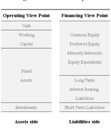
(27) 3.2.1. Invested Capital The invested capital (IC) is the amount of money that holders and shareholders have committed to the company. Basically, and given the concept of EVA, it is the amount of money invested in the company for which management has to produce a return. IC (using an operating approach) can be estimated by subtracting all non-interest-bearing current liabilities (net working capital) from total liabilities and total equity (or total assets). In other words, IC is the sum of fixed (tangible and intangible) assets, plus investments, cash and working capital requirements. This was our first approach to the estimation of IC. However, due to the lack of relevant data and detailed information to properly compute working capital, our estimations were distorted. Thus, we decided to follow an alternative methodology as suggested by Stewart (1991) and reinforced by Roztocki and Needy (1999). According to these authors, a simpler way to estimate a company’s IC is to sum all of its financial sources, such as short-term debt and long-term debt, and owners’ equity. This methodology is considered the most simple, since we only need the liabilities’ side of the balance sheet1. Hence, IC in each firm is the sum of shareholders’ equity plus total liabilities, net of non-interest-bearing short-term liabilities, i.e. amongst the total current liabilities we have only considered short-term financial debt. Even though the companies present in our sample were not affected by such conditions, one must be attentive of the long term non-interest-bearing liabilities. For those calculating EVA, provisions, deferred taxes and minority interests should be considered equity equivalents and taken into account for the necessary adjustments.. 3.2.2. Cost of Capital Our next step was to compute the average cost of capital. Typically, companies resort to two sources of financing: using shareholders’ and investors’ capital, which translates into equity, 1All. the money on the liabilities side of the balance sheet is money committed to the company, although part of it was not actually invested in the company with the purpose of obtaining a return. Included in this later case, are accounts payable to suppliers, money owed to employees or to the state and other short term liabilities, with the exception of short-term debt.. 19.

(28) Figure 3.2: Invested Capital. Figure 3.2 shows a comparison between the two approaches to calculating IC: i) operating view point, using the right side (Assets) or ii) financing view point, using the left side (Liabilities) of the balance sheet.. and borrowing capital from financial institutions (such as banks), which translates into financial debt. Both types of financing have an associated cost, to which we call cost of equity and cost of debt, respectively. The total cost of a company’s financing can be estimated by the weighted average of these two factors (WACC), using the formula:. W ACC = re ×. E D + rd × × (1 − tc ) , IC IC. (3.1). where re represents the cost of equity, rd is the cost of debt, E is the book value of the company’s equity, D is the book value of the company’s financial debt, IC is the invested capital, as a result of (D + E), and tc represents the corporate tax rate, which was obtained via Ministry of Finance’s website. It should be noted that, if the companies in our sample were listed companies, we should use the market values for debt and equity, as the WACC methodology postulates. 20.

(29) Capital structure In what concerns the financial structure of the companies, it is necessary to compute the market value of the firm, and the breakdown between equity and debt. The breakdown between equity and debt should be computed on a market value basis rather than in a book value basis. This is because it is only the market value that truly reflects the cost of funding2. However, as referred above, since the companies present in our sample are not listed companies, we have to use the companies’ capital structure weightings on a book value basis, and assume it as a proxy value for its possible market value. In a survey by Weaver (2001), the author asked 30 companies whether they look at the capital structure weightings on a book or market basis. Fourteen companies used market weights, compared to eleven companies that used book weights (the remaining five companies did not answer). It should be noted that allowances for guarantee, doubtful accounts, contingency values, deferred taxes and (possible) minority interests were implicitly included in the equity book value.. Cost of debt The average cost of debt may be estimated using the yield to maturity of the company’s bond issues or through the use of debt rating tables. Likewise the capital structure weightings, the cost of debt should be the market cost of debt, i.e. the cost that the company would have to pay so as to issue new debt3. Because we do not have market values for the debt of the companies in our sample, the cost of debt was estimated through the ratio of interest paid and the amount of financial debt for each year and, therefore, we considered the cost of debt as an average interest rate.. Cost of equity The cost of equity is very difficult to observe as it is the return demanded by the market for a stock with a risk similar to the company being evaluated. It is common practice to use the 2For. instance, if a company wants to change its financial structure to, suppose, increase the weight of debt and reduce the weight of equity, it will have to issue bonds at market prices and/or repurchase stocks at market prices. Thus, weighting the cost of capital with market values is the only way to obtain the true cost of capital. 3This is the actual opportunity cost for bond holders, and thus is what they are expecting to obtain by investing their money in similar risk projects.. 21.

(30) Capital Asset Pricing Model (CAPM) to estimate the cost of equity. In fact, Weaver (2001) reported in his survey that 29 of the 30 companies employ CAPM to estimate their cost of equity. The CAPM model postulates that the cost of equity is computed as the sum of the risk free rate, plus a risk premium that depends on the market risk premium and a beta coefficient that reflects the systematic risk of the company.. re = rf + β L × (rm − rf ) ,. (3.2). where rf is the risk free rate, β L is the levered beta and (rm − rf ) represents the market risk premium. Risk Free Rates. As the risk free rate is observable in the yield to maturity of long term government bonds, for each year we used the one year yield benchmark for the Eurozone, obtained via Bloomberg. Now, we are left with the problem of estimating the market risk premium and the beta of the company. Market Risk Premium. The market risk premium, at first calculated by the difference between the Eurozone stockmarket benchmark (STOXX600) and the the riskless rates for the Eurozone (treasury bills with one year maturity), as mentioned in the above paragraph. However, given the high volatility of the values that we have obtained, highly influenced by the uncertainty of the economical and financial environment experienced all across Europe, we have decided to use an alternative approach, resorting to the work of Professor Pablo Fernandez, from IESE Business School (Fernandez, Aguirreamalloa and Linares (2013), Fernandez and Del Campo (2010)). Professor Fernandez conducted several studies on equity risk premium, based on surveys sent to different professionals of the economic and financial areas (professors, risk analysts, managers of companies and managers of financial companies) aiming to produce a sensible estimate for the market risk premium of several European countries, including Portugal. As displayed in Table 3.5, the effectively used values for the market risk premium in the years of 2008, 2009 and 2010 are 5.3%, 5.3% and 5.15%, respectively. The market risk premium 22.

(31) Table 3.5: Estimates for the market risk premium 2008 -52.70% 5.30% 5.30%. Author’s estimates (STOXX600) Fernandez et al. (2013) Values Effectively Used. 2009 2010 23.42% 6.34% 5.30% 5.3% and 5% 5.30% 5.15%. Table 3.5 shows the estimates for the market risk premium collected from different sources. The first line shows the author’s estimates based on the difference between STOXX600 benchmark and the risk free rate; the second line shows the estimates obtained from Fernandez et al. (2013). Both lines refer to European market risk premiums. The third line reports the effectively used estimates for the market risk premium, in the years 2008, 2009 and 2010; the 2010 estimate results from the average between 5.3% and 5.15%.. for the year 2010 is an average of the results found by Fernandez et al. (2013) in the surveys made to both professors (5.3%) and risk analysts (5%) for the European risk premium. Professor Fernandez has also estimated the market risk premiums for Portugal. However, since we are using the European MSCI Index as a benchmark, for a matter of consistency, the estimates for Europe were the most appropriate values to use. The adjustments for the Portuguese context will be made through the levered betas. Company’s systematic risk (beta). The best way to obtain an estimate of the companies’ levered beta is to use past stock return information and regress it versus the local market. For companies not listed, the best way to calculate a beta is to start with a beta of a company operating in the same line of business and adjusting it for possible differences in capital structure. This process was, amongst all the components needed for the cost of capital, the most complex and, for simplicity’s sake, can be decomposed in several steps. Since we did not have comparable companies, we had to use the sectorial information to proxy the average risk of a company operating in that sector. Due to the absence of historical information with sufficient depth on the betas for each sector of activity in Portugal (even in the cases where there was some historical depth, it only went as far as a year or two in time), we had to estimate them. Step 1: We started by collecting the monthly values for the MSCI Index for the European activity sectors. This step consisted in regressing the sectorial returns versus the market portfolio returns via the market model4 to obtain the sectorial levered betas, assuming as the 4The. market model used was rii = αi + β i × rmi + εit , 23.

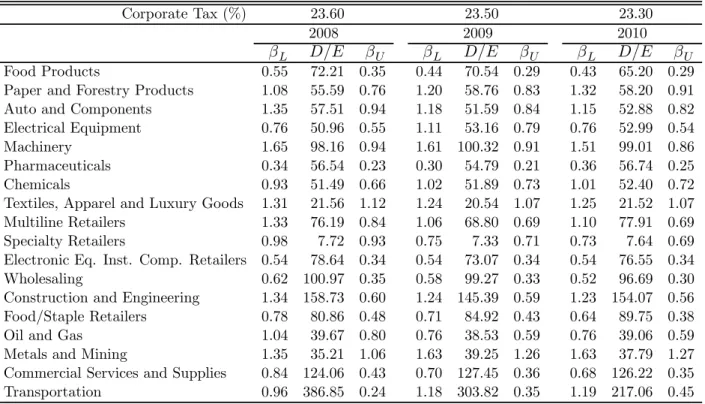
(32) market portfolio the MSCI Europe Index. We chose the MSCI Europe Index as a market portfolio mainly for three reasons: first, it is calculated based on the weighted average of the stock prices; second, it is a benchmark that incorporates income generated from the distribution of dividends and, finally, it is a geographically diversified index, as it incorporates in its composition shares from companies scattered from all across Europe. Step 2: After computing the levered beta for each sector, two procedures are necessary for the betas to reflect different capital structures. First, we had to unlever the betas, which means we had to calculate the beta of the company as if it had no debt. In order to do so, we used annual averages of debt-to-equity ratios for each sector5 , obtained via Bloomberg. For this same purpose, we used income corporate taxes in effect, collected from Eurostat6 . Table 3.6 displays the estimates of the levered betas, debt-toequity ratios and the implicit unlevered betas of the European sectors for years of 2008, 2009 and 2010. Without getting into much technical detail, the unlever and re-lever of the beta can be done through the equation 3.37 . For more details, please see Hamada (1972).. βU =. βL 1 + (1 − tc ) ×. D E. ,. (3.3). where β U and β L are the unlevered and levered betas, respectively, E is the book value of equity and D is the book value of debt (assumed here as proxies for their respective market values); tc is the corporate tax rate. Since the estimated unlevered betas reflect the average risk for the European sectors, which are much lower than those in Portugal, it was necessary to make another adjustment, through the estimation of a country risk coefficient for Portugal8. where rmi , rii are the logatithmic rates of return for the market m and the sector i, respectively, αi is the the component of the return that is independent of the market’s behavior, β i is the levered beta for the sector i and εit is the residual estimation error, which we assume that has an expected value of zero and homoscedastic variance. 5 The annual debt-to-equity ratios used were computed based on the trimestral debt-to-equity ratios for each year, obtained directly via Bloomberg. 6 The corporate tax rates were retrieved from an Eurostat report Eurostat (2011). 7 The beta that reflects the debts’ risk for the sector was considered zero, simulating the most neutral situation possible. 8The purpose of this risk coefficient aims to proxy the risk of Portugal, compared to the risk of other Eurozone countries. It was computed based on the 5 year maturity yields for these same countries.. 24.

(33) Table 3.6: Levered and unlevered beta for the European sectors Corporate Tax (%). Food Products Paper and Forestry Products Auto and Components Electrical Equipment Machinery Pharmaceuticals Chemicals Textiles, Apparel and Luxury Goods Multiline Retailers Specialty Retailers Electronic Eq. Inst. Comp. Retailers Wholesaling Construction and Engineering Food/Staple Retailers Oil and Gas Metals and Mining Commercial Services and Supplies Transportation. 23.60 2008. 23.50 2009. 23.30 2010. βL. D/E. βU. βL. D/E. βU. 0.55 1.08 1.35 0.76 1.65 0.34 0.93 1.31 1.33 0.98 0.54 0.62 1.34 0.78 1.04 1.35 0.84 0.96. 72.21 55.59 57.51 50.96 98.16 56.54 51.49 21.56 76.19 7.72 78.64 100.97 158.73 80.86 39.67 35.21 124.06 386.85. 0.35 0.76 0.94 0.55 0.94 0.23 0.66 1.12 0.84 0.93 0.34 0.35 0.60 0.48 0.80 1.06 0.43 0.24. 0.44 1.20 1.18 1.11 1.61 0.30 1.02 1.24 1.06 0.75 0.54 0.58 1.24 0.71 0.76 1.63 0.70 1.18. 70.54 58.76 51.59 53.16 100.32 54.79 51.89 20.54 68.80 7.33 73.07 99.27 145.39 84.92 38.53 39.25 127.45 303.82. 0.29 0.83 0.84 0.79 0.91 0.21 0.73 1.07 0.69 0.71 0.34 0.33 0.59 0.43 0.59 1.26 0.36 0.35. βL. D/E. βU. 0.43 65.20 0.29 1.32 58.20 0.91 1.15 52.88 0.82 0.76 52.99 0.54 1.51 99.01 0.86 0.36 56.74 0.25 1.01 52.40 0.72 1.25 21.52 1.07 1.10 77.91 0.69 0.73 7.64 0.69 0.54 76.55 0.34 0.52 96.69 0.30 1.23 154.07 0.56 0.64 89.75 0.38 0.76 39.06 0.59 1.63 37.79 1.27 0.68 126.22 0.35 1.19 217.06 0.45. ¡ ¢. Table 3.6 displays the estimates of the levered betas (β L ), debt-to-equity ratios D E and the implicit unlevered betas (β U ) of the European sectors for years of 2008, 2009 and 2010, computed using equation 3.3 and assuming that beta of debt (β D ) is zero.. Godfrey and Espinosa (1996) suggested a method in which we could add the country default spread to the risk free rate and multiply the European risk premium by the volatility of the company’s equity market relative to the European market. Due to the significant correlation between the European and the Portuguese markets, this method did not seem to be the best way to introduce the country market risk premium. Thus, we tried to find alternative methods to incorporate the country market risk premium in the cost of equity. We chose to estimate the country risk premium as a spread over the benchmark treasury yield. For each country, the sovereign risk premium was computed as the spread between its sovereign five year yield and the Eurozone benchmark yield for the same maturity. After estimating the sovereign risk premium for each country, we were able to calculate an average of the sovereign risk premium, which we will consider as the European risk premium. Finally, the country risk coefficient for Portugal is the ratio between the Portuguese risk premium and the average Eurozone sovereign risk premium. This risk coefficient, as displayed in Table 3.7, 25.

(34) will be used to adjust the European unlevered betas into the Portuguese unlevered betas for each sector. Table 3.7: Estimates for country risk coefficient. (1) Portuguese risk premium (b.p.) (2) European risk premium (b.p.) (3) = (1) / (2) Coefficient risk premium. 2007 8 10 1.23. 2008 58 46 1.24. 2009 220 215 1.02. 2010 381 282 1.35. Table 3.7 shows the risk coefficient that will be used to estimate the unlevered betas (β U ) for Portuguese sectors. The Portuguese risk premium is the difference between the Portuguese five year yield and the five year European benchmark; Europe risk premium is the difference between the average of the five year yields of the Eurozone countries and the European benchmark. The European benchmak considered is the Bloomerg’s European sovereign five year yield index.. As observed in Table 3.7, Portugal has followed the increase tendency of Eurozone’s spread over the five year yield sovereign benchmark, increasing from 10 b.p. in 2007 to 282 b.p. in 2010. Regarding the Eurozone countries, the five year yield average spread rose from 8 b.p. in 2007 to 381 b.p. in 2010. This evolution is particularly influenced by the increase in credit spreads, not only in Portugal, but also in countries such as Greece and Ireland, due to the economic and financial bailout in 2010. The Portuguese coefficient risk premium, which was relatively stable during the years of 2007 and 2008, has decreased to 1.02 in 2009 and registered an increase to 1.35 in 2010. Secondly, we had to re-lever the beta, i.e. we had to recalculate the levered betas, starting from the unlevered beta that reflects the assets’ average risk for a company and adjusting for the capital structure of each company, in each sector. This process was guided by Damodaran (2001) bottom-up betas approach.. 3.2.3. Return on Invested Capital As WACC reflects the average capital charges, the return on invested capital (ROIC) reflects the return on capital employed in the business. ROIC was computed based on equation 3.4:. ROIC =. EBIT (1 − tc ) , ICboy 26. (3.4).

(35) Table 3.8: Estimated unlevered betas: Europe and Portugal. Food Products Paper and Forestry Products Auto and Components Electrical Equipment Machinery Pharmaceuticals Chemicals Textiles, Apparel and Luxury Goods Multiline Retailers Specialty Retailers Electronic Eq. Inst. Comp. Retailers Wholesaling Construction and Engineering Food/Staple Retailers Oil and Gas Metals and Mining Commercial Services and Supplies Transportation. 2008. 2009. 2010. β U Eur β U Prt. β U Eur β U Prt. β U Eur β U Prt. 0.35 0.76 0.94 0.55 0.94 0.23 0.66 1.12 0.84 0.93 0.34 0.35 0.60 0.48 0.80 1.06 0.43 0.24. 0.44 0.94 1.17 0.68 1.17 0.29 0.83 1.40 1.05 1.15 0.42 0.43 0.75 0.60 0.99 1.32 0.54 0.30. 0.29 0.83 0.84 0.79 0.91 0.21 0.73 1.07 0.69 0.71 0.34 0.33 0.59 0.43 0.59 1.26 0.36 0.35. 0.29 0.85 0.86 0.81 0.94 0.22 0.75 1.10 0.71 0.73 0.35 0.34 0.60 0.44 0.60 1.29 0.36 0.36. 0.29 0.91 0.82 0.54 0.86 0.25 0.72 1.07 0.69 0.69 0.34 0.30 0.56 0.38 0.59 1.27 0.35 0.45. 0.39 1.23 1.11 0.73 1.16 0.34 0.97 1.44 0.93 0.93 0.46 0.40 0.76 0.51 0.79 1.71 0.47 0.61. Table 3.8 exhibits the unlevered betas estimated for the European sectors and Portuguese sectors, which were adjusted by the Portuguese country risk coefficient, shown in Table 3.7. “β U Eur” refers to the unlevered betas of the European sectors and “β U Prt” refers to the unlevered betas of the Portuguese sectors.. where EBIT corresponds to the earnings before interest and taxes, tc is the corporate tax in effect for the period and ICboy is the invested capital at the beginning of the year. 3.2.4. Economic Value Added Having calculated the three main components needed in order to estimate EVA, we have now gathered all the information we need so as to proceed with our work. To do so, we have applied equation 3.5.. EV A = (ROIC − W ACC) × ICboy .. (3.5). Equation 3.5 was applied to all the companies, providing an estimate for each company’s EVA, in absolute terms. Because the companies present in our rankings belong to very different sectors, with a very different set of financial and economic characteristics, these values were hardly comparable and might lead us into taking the wrong conclusions. In order to have 27.

(36) comparable data between companies from different sectors and different time spans, we decided to use a different indicator, to which we called EVA spread that, because of its relative nature, allowed us to make the comparisons needed between companies, in order to estimate the best performances in each year and between each sector of activity.. EV A Spread = ROIC − W ACC.. (3.6). As shown in the equation 3.6, EVA Spread is easy to compute as it is given by the difference between the return on invested capital and the weighted average cost of capital.. 3.2.5. Market Value Added According to Dierks and Patel (1997), the Market Value Added (MVA) is an indicator, in absolute terms, of a company’s created wealth for its investors over a period of time. The computation of the MVA is as simple as the sum of the EVAs registered over a certain period of time, as in equation 3.7: n X EV At , MV A =. (3.7). t=1. where MV A is the Market Value Added and EV At is the estimated Economic Value Added for the year t. So, in our case, MVA is the sum of EVAs for 2008-2010 period. As in the previous indicator, EVA, there was a need to adapt MVA, which gave us absolute values that might distort our conclusions. Thus, we decided to transform the absolute MVA into a relative basis, as shown by equation 3.8.. RMV A =. MV A , n P 1 ICt n. (3.8). t=1. The Relative MVA (RMVA) is estimated by dividing a company’s MVA for a period of time t, by the average of its IC during the same period (in our sample 2008-2010, or better 28.

(37) 2007 2009 since IC is lagged — i.e., it refers to the beginning of the year, which is the same as the end of the previous year). 3.3. EVA accounting adjustments The adjustments recommended by authors such as Stewart (1991), Young (1999), Weaver (2001), Correia et al. (2007) and Drury (2007) should be made only if the four following criteria, as mentioned in section 2.4, are met: i) the amounts considered are significant; ii) they are likely to have a material influence; iii) operational level employees can easily understand them; and iv) the required information is easily tracked. These criteria are utmost important when one is dealing with companies with a divisional structure. The more complex the structure, the greater the possible distortions made by the application of GAAP. In order to apply these adjustments, one must have access to the internal accounting, financial and other managerial information. Since the present dissertation aims to measure the value created by the Portuguese SME, using a representative sample of 315 companies, evaluating the adequacy of these criteria to each company would be virtually impossible. The computation of EVA, according to equation 3.5, which seems straightforward and simple, was applied to all the 315 companies in the sample. However, we decided to take on some assumptions that aimed to approximate the available information to the economic reality. Such assumptions were i) EBIT after taxes as a proxy for NOPAT; ii) IC–as a result of the sum of the book value of the company’s equity and the book value of the company’s financial debt, only reflects the value of the assets in place; iii) the discretionary expenses such as research and development and market, and advertising are implicitly included in the IC; iv) the owners’ loans were considered as financial debt; v) financial leasings were also considered as part of the financial debt, by the inclusion of the accounting item fixed asset suppliers; and vi) non-recurrent gains and losses were not considered9. 9According. to Frezati (2003), single events whose repercussion on income only occurs at a specific moment in time, should not be included in the computation of income. Van der Poll et al. (2011) also noted that, in what concerns NOPAT, non-recurrent gains and losses should not be included in the EVA computation. In our sample, the non-recurrent gains and losses represent about 20% of the taxable income.. 29.

(38) Adjustments that relate to i) the goodwill and respective amortization; ii) deferred taxes iii) depreciation methods; iv) inventory valuation methods; v) allowance for guarantee, doubtful accounts and contingency are also relevant, however they were not considered in the computation of EVA due to the lack of information. Chapter 4 presents the empirical results of the EVA calculation for the sample of 315 biggest and best Portuguese SME.. 30.

(39) CHAPTER 4. PERFORMANCE ASSESSMENT RESULTS In this chapter, we report the results of our performance assessment, as measured by EVA and MVA, of the 315 SME analyzed in our sample for the period 2008 2010. Table 4.1 summarizes these results. Table 4.1: Summary of EVA and MVA results Panel A: EVA Number of companies with Sum of negative EVAs Number of companies with Sum of positive EVAs Total EVA Panel B: MVA Number of companies with Sum of negative MVAs Number of companies with Sum of positive MVAs Total MVA. negative EVA positive EVA. negative MVA positive MVA. 2008 216 -119,646 99 39,878 -79,769. 2009 2010 197 157 -96,795 -79,118 118 158 46,971 70,681 -49,824 -8,437 2008 - 2010 200 -262,968 115 124,938 -138,029. Table 4.1 exhibits the results of the performance assessment, as measured by EVA and MVA, of the 315 SMEs analyzed in our sample for the period 2008 2010.. Globally, the total EVA is negative in each of the three years. The total sum of negative EVAs is -119,646k€ in 2008, 96,795k€ in 2009 and -79,118k€ in 2010. However, the number of companies with negative EVA decreases by each year, from 216 companies in 2008, to 197 companies in 2009, to 157 companies in 2010. In line with these results, the number of companies with negative MVA is 200, amounting to -262,968k€. The total MVA is negative and adds up to -138,029k€. In section 4.1 we analyze the three main EVA components and the results of the EVA evaluation, as presented in subsection 3.2.4, equation 3.5. In section 4.2, we try to answer our investigation question “Did the biggest and best Portuguese SME create value during the first three years of the crisis period of 2008 2010?" by examining MVA and RMVA estimated for 31.

(40) the whole sample, and detailed by sector. Finally, in section 4.3 we rank the ten companies with the best and worst performances, measured in terms of EVA Spread and RMVA.. 4.1. EVA components and EVA Spread analysis Table 4.2 displays the descriptive statistics for the three main EVA components, as well as our estimates of EVA and EVA Spread. Panel A, Panel B and Panel C present the global figures for the years of 2008, 2009 and 2010, respectively.. Table 4.2: Descriptive statistics for EVA main components (2008, 2009 and 2010). Panel A: 2008 Average Std Deviation 1st Quartile 2nd Quartile 3rd Quartile Maximum Minimum Panel B: 2009 Average Std Deviation 1st Quartile 2nd Quartile 3rd Quartile Maximum Minimum Panel C: 2010 Average Std Deviation 1st Quartile 2nd Quartile 3rd Quartile Maximum Minimum Representative company. EVA. EVA Spread. WACC. ROIC. IC. 9.23% 2.96% 7.22% 8.84% 10.59% 24.73% 4.46%. 6.39% 14.25% 1.22% 5.14% 11.21% 62.29% -78.85%. 6,584 5,129 2,648 5,310 8,840 28,807 386. -253 -2.84% 732 14.50% -499 -8.14% -151 -3.26% 74 1.60% 3,284 56.20% -4,347 -103.58%. 6.68% 2.84% 5.01% 6.36% 7.57% 34.28% 2.63%. 5.05% 11.31% 1.28% 4.53% 8.79% 51.43% -88.74%. 7,642 5,925 3,132 6,131 10,246 34,464 351. -158 685 -421 -78 114 2,249 -3,311. -1.13% 11.62% -5.84% -2.07% 2.42% 45.97% -99.84%. 5.10% 1.80% 3.44% 4.88% 6.29% 11.88% 1.80%. 6.21% 11.43% 1.62% 4.98% 9.21% 71.48% -57.21%. 7,716 5,892 3,038 6,341 10,108 33,524 421. -27 734 -324 0 242 3,333 -4,375. 2.67% 11.89% -4.45% 0.00% 4.80% 69.68% -60.26%. 7.00%. 5.88%. 7,314. -146. -0.43%. Table 4.2 displays the descriptive statistics for the three main EVA components, as well as our estimates of EVA and EVA Spread. Panel A, Panel B and Panel C present the global figures for the years of 2008, 2009 and 2010, respectively. The representative company refers to a theoretical company, which portraits as the average SME of our whole sample. The EVA components for the representative company result of the sum of each year’s average EVA components.. 32.

(41) When comparing the results of the three panels, there was a straight decrease in the average WACC from 9.23% in 2008 to 5.10% in 2010. Considering the three years, the maximum observed value was 34.28% in 2009 and the minimum was 1.80% in 2010. Regarding ROIC, there was no specific tendency noted for the evolution of this variable. In fact, and in average terms, there was a reduction in 2009 and an increase in 2010. The observed evolution may have its justification in the fact that, from 2008 to 2009, both EBIT and IC showed, however positive, a disproportionate variation–that is, IC grew about 3 times more than EBIT. By contrast, between 2009 and 2010, EBIT’s growth was more accentuated than that of the IC, reflecting an increase in ROIC over the referred period. The evolution of IC was, for the three years, relatively homogeneous for the three quartiles. The average EVA estimated for the companies in our sample was negative, in all three years. However, as presented in Table 4.2 this variable displays a continuous and significant improvement during the three year period. In fact, the average EVA was -253k€ in 2008, -158k€ in 2009 and -27k€ in 2010. The maximum and minimum EVA values were observed in 2010, 3,333k€ and -4,375k€, respectively. In 2008 and 2009, more than half the companies of our sample reported a negative EVA. In 2010, 50% of the companies reported a negative EVA. The difference, in terms of EVA, between the best company in the first quartile and the worst in the third quartile was, on average, approximately 550k€. Table 4.3 presents a deeper insight on the companies’ weighted average EVA components in a sectorial perspective for the years of 2008, 2009 and 2010. All the components are weighted by each sector’s IC. Since EVA Spread reflects the difference between ROIC and WACC, the behavior of this variable is a direct consequence of the combination of the last two. The difference registered between the average EVA and average EVA Spread lies in the different levels of invested capital by each sector. This means that the true economic profit, as described by Dierks and Patel (1997), reflects how well each sector can capitalize their investments, after deducting all the costs inherent to the business. Thus, the analysis of Table 4.3 is going to be made, essentially, in an EVA Spread perspective.. 33.

(42) Table 4.3: EVA main components by sector (2008, 2009 and 2010) 2008 Food Products 3.39% Paper and Forestry Products 0.63% Auto and Components 1.21% Electrical Equipment 1.80% Machinery 2.27% Pharmaceuticals 1.04% Chemicals 1.81% Textiles, Apparel and Luxury Goods 2.91% Multiline Retailers 4.45% Specialty Retailers 0.06% Electronic Eq. Inst. Comp Retailers 3.11% Wholesaling 3.45% Construction and Engineering 3.70% Food/Staple Retailers 8.06% Oil and Gas 2.93% Metals and Mining 1.50% Commercial Services and Supplies 2.23% Transportation 3.51%. WACC 2009 3.68% 0.69% 0.41% 1.53% 2.03% 0.08% 2.02% 2.87% 4.67% 0.40% 2.72% 2.33% 3.29% 4.21% 2.74% 0.93% 0.97% 2.09%. 2010 4.61% 0.49% 0.25% 1.01% 0.75% 1.94% 0.73% 1.28% 3.75% 1.05% 2.20% 3.36% 3.68% 6.70% 2.37% 0.90% 1.08% 1.80%. 2008 7.99% 1.51% 0.92% 1.16% 2.12% 1.18% 2.32% 5.80% 8.91% 6.62% 2.27% 4.50% 5.94% 9.66% 3.71% 1.65% 1.58% 1.60%. ROIC 2009 5.09% 1.10% 0.72% 0.94% 1.83% 1.02% 1.78% 4.11% 5.91% 4.66% 1.57% 2.93% 4.48% 7.38% 2.72% 1.35% 1.10% 1.19%. 2010 3.29% 0.94% 0.50% 0.60% 1.08% 0.26% 1.18% 2.76% 3.95% 3.21% 0.98% 1.68% 3.15% 3.35% 1.75% 1.09% 0.65% 0.75%. IC 2008 8,361 12,123 12,436 9,785 12,068 5,963 11,019 5,936 4,157 6,519 5,617 7,781 8,208 3,377 2,446 8,673 3,447 6,383. (’000 EUR) 2009 2010 9,451 9,742 12,358 12,702 14,711 14,632 10,974 11,317 15,514 15,693 6,901 4,654 12,244 12,039 7,103 7,481 5,350 5,654 7,381 7,271 6,349 6,239 8,389 8,571 10,283 10,456 3,966 3,893 2,750 2,693 9,716 9,777 4,214 3,987 7,065 7,066. EVA Spread 2008 2009 2010 -4.60% -1.41% 1.32% -0.88% -0.41% -0.44% 0.29% -0.31% -0.25% 0.64% 0.59% 0.40% 0.15% 0.20% -0.33% -0.14% -0.94% 1.69% -0.51% 0.24% -0.45% -2.89% -1.24% -1.47% -4.46% -1.25% -0.20% -6.56% -4.25% -2.15% 0.83% 1.15% 1.22% -1.05% -0.59% 1.69% -2.24% -1.19% 0.53% -1.59% -3.17% 3.35% -0.78% 0.03% 0.62% -0.14% -0.42% -0.19% 0.65% -0.13% 0.43% 1.91% 0.89% 1.04%. Table 4.3 displays the companies’ weighted average EVA components in a sectorial perspective for the years of 2008, 2009 and 2010. All the components are weighted by each sector’s IC. Since EVA Spread reflects the difference between ROIC and WACC, the behavior of this variable is a direct consequence of the combination of the last two. The difference registered between the average EVA and average EVA Spread lies in the different levels of invested capital by each sector.. 34.