Coastal Responses to sea-level rise on centennial to
millennial time scales: development of hybrid
model-based forecasting for the Guadiana Estuary
Dissanayake Mudiyanselage Ruwan Sampath
Doutoramento em Ciências do Mar, da Terra e do Ambiente,
Ramo de Geociências, Especialidade em Dinâmica Litoral
Coastal Responses to sea-level rise on centennial to
millennial time scales: development of hybrid
model-based forecasting for the Guadiana Estuary
Dissanayake Mudiyanselage Ruwan Sampath
Doutoramento em Ciências do Mar, da Terra e do Ambiente,
Ramo de Geociências, Especialidade em Dinâmica Litoral
Tese Orientada por:
i
the mankind, unfortunately, whose relentless exploitations of the Mother Nature due to their
selfish greediness have been endangered not only the survival of themselves but the very
existence of the whole world.
To my parents, Sirisena and Ramani,
My wife Nadeesha
My sister Ruwani,
For supporting me unconditionally,
Even when I do nothing but my studies.
“The cold remote islands
And the blue estuaries
Where what breathes, breathes
The restless wind of the inlets,
And what drinks, drinks
The incoming tide.”
ii
“Solving a problem for which you know there’s an answer is like climbing a mountain with a guide, along a trail someone else has laid…..
The truth is somewhere out there in a place no one knows, beyond all the beaten paths. And it’s not always at the top of the mountain.
It might be in a crack on the smoothest cliff or somewhere deep in the valley.” ― Yōko Ogawa
iii
Since bachelors years, I had a dream of doing a doctoral degree and then to engage in my own research carrier to explore a few things to my interest in the environmental engineering and science field. Sometimes I was distracted a bit, but I was able to realign my focus. Now I think I have reached very near to that goal. It was not a smooth or direct path, but decorated with numerous hardships and sacrifices. Despite all these obstacles, I was able to move forward inch by inch along this path due to generous helps, encouragement, and continuous guidance by a few people who are with me altogether.
The first name that I remember with a lot of gratitude and respect is my supervisor Prof. Tomasz Boski, at the University of Algarve. First, I would like to express my sincere appreciation to him, for his continuous guidance and unwavering support. He even supervised me during my Erasmus Mundus Master’s degree in Water and Coastal Management. I discussed with him so many ideas to improve the scope of the thesis. Sometimes some of them have to be abandoned due to logistical and practical reasons. Yet, I could always count on his help to carry out this doctoral study. Many times he gave me a good opportunity to explore my own ideas. Prof. Tomasz´s attention to all aspects of a student life, in particular of a foreign student is very remarkable. I was able to solve not only the academic problems, but also the personal issues arisen due to lots of reasons. I can remember forever, how he helped me to overcome financial issues when my father was required to undergo a bypass surgery. He also helped me in a lot of ways when I suffered from a disease for a long time. If I did not have those assistance, I may not be able to do this study successfully. Thus, I would like to thank for him for everything. I also would like to thank Prof. Alice Newton during this study. She sent me important research papers for my study whenever she comes across one. She gave me valuable guides whenever I met her at the University of Algarve or at the University of Cadiz. She is also a mentor to me in numerous ways during this study period.
iv
from 2007. He helped me to work with models, ARCGIS and other academic activities. I was always able to count on him for whatever assistance that I required during these 8 years. Carlos Sousa too helped me in numerous ways to solve issues with ARCGIS, creating graphics and for field work. Erwan Garel and Carlos Sousa helped me to carry out the bathymetric surveying, finding data from various Portuguese sources. Ana Gomes helped me to sort out some of the academic issues related to the Academic Service of the University of Algarve. Carlos Loureiro, Carlos Sousa and Ana Gomes helped me to get some of the sections translated into Portuguese. Laura Ferreira and Bruno Fragoso also helped me in many ways. I was so very warmly welcome by everyone in the Centro de Investigação Marinha e Ambiental (CIMA) at the University of Algarve. It didn’t take long to feel like I was a member of the family of CIMA. The atmosphere in the CIMA group was great and I would like to thank everyone including Zélia Coelho.
Since my childhood, I received a strong support and encouragement for academic activities from my parents Sirisena and Ramani and sister. They avoid me from a lot of distractions. The encouragements by my wife Nadeesha and her parents and siblings to focus strictly on my academic work have been fundamental. She always reminds me that I have to forget all the other things, but to spend time for study. I would like to thank especially my sister for looking after our parents, which is my obligation. Finally, I would like to thank everyone at the University of Algarve for their kind attention and helps when a need arise.
This research was possible through the financial support of:
Ph.D grant by Fundação para a Ciência e Tecnologia (SFRH/BD/70747/2010) Research grant by Centro de Investigação Marinha e Ambiental (UID/MAR/
vi
In the context of hybrid approach, this study was focused on formalizing and application of a simple and idealized model using a set of theoretical framework based on rule-based morphological expressions. Main objectives were: (1) to simulate the sedimentary infilling of the Guadiana Estuary palaeovalley due to eustatic sea-level rise during the Holocene, against previous geomorphological and post-glacial palaeoenvironmental reconstructions based on facies interpretation and 14C dating; (2) to assess potential morphological impacts and risk of
habitat shift by simulating the morphological evolution of the Guadiana estuary and its intertidal zone for the worst case of sea level rise and sedimentation scenarios predicted for the 21st century; (3) to assess the sensitivity of bed friction coefficient, power index of the current velocity in the erosion rate function, river discharge, and sea-level rise rate in determining the decadal scale morphological evolution in the Guadiana estuary; and (4) To understand the effect of dam construction along the Guadiana river on the estuarine morphology.
According to the results, the long-term modelling of the morphological evolution in the estuary due to sea-level rise during the Holocene complemented previous reconstructions, based on interpretations of the experimental data. The intermediate hybrid approach that was followed in this study appears to be a useful tool for simulating the morphological evolution of an estuarine system during the period of postglacial sea-level rise. It seems particularly suited to the more sheltered environments of an estuarine system where vertical aggradation dominates the sedimentary infilling of the palaeovalley. However, the direct application of Estuarine Sedimentation Model and the intermediate hybrid model, are very much applicable to a system where there is net accretion throughout the estuarine system. These constraints were compensated to a certain extent using the fully developed hybrid model as it was able to produce elevation change distribution from 2000 to 2014 in the Guadiana estuary, approximately similar to the observed normal probability distribution for the same period. This
vii
enabling the coupling of decadal scale model to centennial scale model. Furthermore, results indicate the deficiencies of defining the environmental flow as a percentage of dry season flow and the risk of habitat loss from the intertidal zone. Thus, a multi-dimensional approach has to be adopted to mitigate their consequences of sea-level rise and drastic flow regulations on the ecosystem of the Guadiana estuary.
Keywords: Estuaries, Sea-level rise, Long-term morphological evolution, Behaviour-oriented models, Hybrid models Hindcasting and forecasting
viii
No contexto de uma abordagem híbrida, este estudo focou-se na formalização e aplicação de um modelo simples e idealizado baseado no enquadramento teórico resultante de expressões geomorfológicas. Os objetivos principais foram: (1) simular o preenchimento sedimentar do palaeovale do estuário do Guadiana devido à subida eustática do nível do mar durante o Holocénico, considerando reconstruções geomorfológicas e pós-glaciais palaeoembientais por sua vez baseadas em interpretação de fácies e datações por Carbono-14; (2) avaliar os potenciais impactos morfológicos e de risco de mudança de habitats através da simulação fa evolução morfológica do estuário do Guadiana e respetiva zona intertidal de acordo com o pior cenário de subida do nível do mar e de sedimentação projetado para o século XXI; (3) avaliar a sensibilidade do coeficiente de fricção de fundo, índice de potência da velocidade de corrente na função de taxa de erosão, e taxa de subida de nível do mar na determinação da evolução morfológica do estuário do Guadiana numa escala temporal de décadas; e (4) perceber qual o efeito na morfologia estuarina da construção de barragens ao longo do rio Guadiana.
De acordo com os resultados obtidos, a modelação a longo prazo da evolução morfológica do estuário devido â subida do nível do mar durante o Holocénico complementou reconstruções prévias baseadas em interpretações de dados experimentais. A abordagem intermédia híbrida seguida neste estudo apresenta-se como uma ferramenta útil para simulação da evolução morfológica de um sistema estuarino durante o período de subida do nível do mar pós-glacial. Torna-se ainda particularmente aplicável a ambientes mais abrigados de um sistema estuarino onde a agradação vertical domina o processo de preenchimento sedimentar do palaeovale. Porém, a aplicação direta do Modelo de Sedimentação Estuarina e do modelo intermédio híbrido é igualmente aplicável a um sistema onde exista acreção generalizada por todo o sistema estuarino. As limitações encontradas foram relativamente compensadas através
ix
elevação do estuário do Guadiana entre 2000 e 2014 de forma aproximadamente semelhante à distribuição normal de probabilidade observada para o mesmo período. Este modelo melhorado permitiu a produção de variabilidade espacial de regiões em acreção e erosão, possibilitando a união entre o modelo operante à escala de décadas com o modelo operante à escala de séculos. Ainda, os resultados obtidos apontam para as limitações na definição de um caudal ecológico como um percentagem do caudal em época seca, e o risco de perda de habitats da zona intertidal. Assim, uma abordagem multi-dimensional deverá ser adotada de forma a mitigar as consequências da subida do nível do mar e da regulação drástica do caudal no ecossistema do estuário do Guadiana.
Palavras-chave: Estuários, Subida do nível do mar; Evolução morfológica a longo prazo; Modelos orientados por comportamento; Modelos híbridos; Reconstrução retrospetiva e preditiv
x
A Humanidade enfrenta grandes desafios no que diz respeito à mitigação e adaptação aos impactos das alterações climáticas globais, incluindo os decorrentes da subida do nível do mar em ambientes estuarinos durante o século XXI. Consequentemente, as autoridades têm que tomar decisões de gestão e implementar políticas que minimizem os riscos de inundação, bem como as ameaças para os habitats estuarinos e costeiros, devido aos cenários que projetam uma subida do nível do mar. Tais impactos negativos podem ser exacerbados devido às atividades humanas intensivas que se desenvolvem nestas regiões. Em contraponto com a abordagem dominante do século XX de mitigar os problemas de erosão costeira com recurso a intervenções intrusivas de engenharia dita “pesada”, que falharam em muitos casos, as aplicações de estratégias de engenharia ditas “ligeiras” têm vindo a ser identificadas como uma abordagem mais sustentável a ser adotada no presente século. Para tal é necessária uma boa compreensão dos processos físicos e biológicos de longo termo, os quais controlam a dinâmica de sistemas estuarinos na sua globalidade. Uma abordagem robusta de modelação terá então que ser considerada para compreender o grau de resposta e sensibilidade de sistemas estuarinos a alterações nos processos dominantes, tais como dinâmica de marés, subida do nível do mar, descarga fluvial e abastecimento sedimentar fluvial. Contudo, a dinâmica sedimentar e, especialmente, as alterações morfológicas de longo-termo são difíceis de modelar, uma vez que a maioria dos modelos de previsão são baseados na simulação de eventos discretos e num insuficiente conhecimento de processos estocásticos.
Apesar de as condições ambientais serem naturalmente diferentes, compreender e simular a evolução estuaria Holocénica em resposta à subida eustática do nível do mar deverá servir como base para prever a sua evolução morfológica durante o século XXI. É ainda importante compreender a incerteza e sensibilidade dos parâmetros de controlo na evolução morfológica durante este século. Existem algumas desvantagens nas abordagens de modelação
xi
híbridos, apesar de estarem ainda numa fase inicial de desenvolvimento, podem combinar o rigor dinâmico de modelos baseados em processos com o conhecimento observacional incorporado em modelos assentes em relações geomorfológicas empíricas ou modelos baseados em comportamentos. Prandle (2004; 2009) desenvolveu uma conceptualização teórica baseada em expressões obtidas a partir de relações morfológicas empíricas, recorrendo à simplificação da equação unidimensional de propagação de momento axial em águas pouco profundas e da equação de continuidade. As teorias daí resultantes fornecem formulações explícitas para as velocidades de corrente, séries temporais de concentração do sedimento em suspensão em função da elevação, alturas de maré, descarga fluvial, dimensão do sedimento, atrito de fundo, erodibilidade e porosidade do sedimento. Desta forma, o modelo híbrido de evolução morfológica está assente nos desenvolvimentos apresentados em Prandle (2004; 2009) e outras relações empíricas obtidas em vários estudos desenvolvidos no sistema estuarino do rio Guadiana.
Para complementar investigações de campo que descreveram a história geomorfológica e a variação do nível do mar ao longo dos últimos 13.000 anos no estuário do Guadiana, localizado no sudoeste da Península Ibérica, foi, no presente estudo, inicialmente aplicado o Modelo de Sedimentação Estuarina de forma a compreender a capacidade e aplicabilidade de uma abordagem de modelação baseada em comportamentos para realizar simulações de longo-termo da evolução morfológica do estuário do Guadiana em resposta às projeções de subida do nível do mar e cenários de défice sedimentar (Capítulo 2). Em segundo lugar, no contexto de uma abordagem híbrida, formalizou-se um modelo simples e idealizado, o qual foi programado em ambiente MATLAB com recurso à conceptualização teórica baseada em expressões morfológicas empíricas obtidas por Prandle (2004; 2009) de forma a:
xii
subida eustática no nível do mar durante o Holocénico (Capítulo 3);
(ii) Avaliar os resultados da modelação em comparação com reconstruções geomorfológicas e paleoambientais pós-glaciais baseadas em interpretação de fácies e datação por radiocarbono – 14C (Capítulo 3);
(iii) Simular a evolução morfológica do estuário do Guadiana e as suas zonas entre marés para os cenários mais gravosos em termos de subida do nível médio do mar e sedimentação previstos para o século XXI (Capítulo 4);
(iv) Analisar os impactos morfológicos potenciais e os riscos de deslocação de habitats por forma a permitir a formulação de políticas de gestão de longo-termo para a totalidade do sistema estuarino (Capítulo 4);
(v) Avaliar a sensibilidade ao coeficiente de atrito de fundo e exponenciação da velocidade da corrente na função da taxa de erosão, bem como a taxa de subida do nível do mar na determinação da evolução morfológica do estuário do Guadiana à escala da década (Capítulo 5);
(vi) Compreender qual o efeito das barragens construídas no longo do Rio Guadiana na morfologia estuarina (Capítulo 5);
(vii) Comparar a taxa de denudação da bacia hidrográfica do Rio Guadiana com recurso ao método isotópico Berílio 10 (10Be) e o método do balanço sedimentar (Capítulo 6); (viii) Avaliar a sensibilidade da descarga fluvial (fluxo ambiental) na evolução morfológica
de longo-termo após a conclusão da barragem de Alqueva em 2002 (Capítulo 7);
Os objetivos 1 a 4 e 7 foram alcançados através da estimação dos coeficientes adimensionais de acreção líquida para um transepto hipotético, compreendido entre o nível máximo de maré alta e a máxima profundidade no estuário do Guadiana, recorrendo-se às expressões
xiii
utilizados para simular a evolução morfológica do estuário do Guadiana usando o Modelo de Sedimentação Estuarina (ESM), o qual representa uma abordagem de modelação numérica orientada por comportamentos morfológicos. Consequentemente, a abordagem implementada no presente trabalho é considerada como uma abordagem híbrida intermédia. As simulações do modelo para os objetivos 5, 6 e 8 foram baseadas no modelo híbrido aperfeiçoado (completamente desenvolvido), o qual estima diretamente a evolução morfológica do estuário do Guadiana de forma a compreender a sensibilidade dos parâmetros de controlo na alteração da elevação em resposta à subida do nível do mar e redução do fornecimento sedimentar. O objetivo 8 servirá para o desenvolvimento de estratégias de gestão de forma a minimizar o impacto da subida do nível do mar e a redução drástica da descarga fluvial devido à construção da barragem de Alqueva.
De acordo com os resultados da aplicação direta do Modelo de Sedimentação Estuarina, durante o século XXI a evolução morfológica do estuário do Guadiana e a sua zona entre marés adjacente são provavelmente melhor representadas pelas projeções que combinam o cenário de subida do nível do mar A1F1 (59 cm) com o cenário de intervenção humana da sedimentação (0.65 mm/ano). Esta combinação de cenários fornece uma percepção ampla do grau de vulnerabilidade do estuário em condições de carência sedimentar. Nestas condições, verificar-se-á um aumento significativo na profundidade efetiva do canal principal. A sedimentação acima do nível médio do mar atingirá apenas 37% do total da sedimentação potencial, o que se deve à exclusividade do forçamento de maré nesta secção. Este valor aumentará até 50, 53 e 57% quando considerado um acréscimo no espaço de acomodação em função de projeções de subida do nível do mar de 38, 48 e 58 cm, respectivamente. A translação horizontal (para terra) do limite superior da zona entre marés do estuário será mais significativa na margem Portuguesa, quando comparada com a mesma translação na margem Espanhola. Nesta última,
xiv
maior risco de desaparecimento de sapais em função do aumento da submergência resultante da subida do nível do mar. Adicionalmente, a translação para terra do nível médio do mar será mais significativa na margem Espanhola, onde os sapais deverão sofrer maior pressão devido à aceleração da subida do nível do mar; este fenómeno deverá ser menos significativo na margem Portuguesa. Em termos gerais, a zona entre marés do estuário do Guadiana deverá aumentar entre 3 a 5% por cada aumento de 10 cm no nível do mar até ao final do século XXI, o que representará uma perda efetiva de terra emersa devido à subida do nível do mar.
Contudo, o modelo em causa é bastante simples e não considera a erosão induzida pelas marés, bem como a variação na descarga fluvial. Consequentemente, este tipo de modelo é muito mais aplicável a sistemas onde se verifica uma acreção efetiva em todo o sistema estuarino. Assim, os constrangimentos na investigação observados em abordagens de modelação orientadas por comportamentos podem ser compensados com a utilização de abordagens híbridas (comportamento-processos), as quais poderão auxiliar na exploração de algumas das vantagens de modelos baseados em processos. Mesmo considerando que este modelo é extremamente idealizado e que os resultados podem conter grandes incertezas, os resultados obtidos podem, pelo menos, indicar a ordem de magnitude dos impactos morfológicos potenciais no sistema estuarino do Guadiana resultantes dos cenários de subida do nível do mar e sedimentação para o século XXI.
Para melhorar a compreensão atual da resposta de sistemas estuarinos a forçamentos naturais, a evolução morfológica do estuário do Guadiana durante o Holocénico, devida à subida eustática do nível do mar, foi simulada com recurso a uma abordagem híbrida intermédia. A modelação de longo termo da evolução morfológica no estuário serviu para complementar reconstruções anteriores, baseadas na interpretação de dados experimentais. As simulações foram realizadas através da estimação dos coeficientes adimensionais de acreção
xv
máxima do estuário do Guadiana, utilizando as expressões matemáticas híbridas de Prandle (2004; 2009). Os coeficientes obtidos foram utilizados para simular a evolução morfológica do estuário do Guadiana utilizando o Modelo de Sedimentação Estuarina (ESM), o qual corresponde a uma abordagem de modelação numérica orientada por comportamentos, e recorrendo-se a uma representação temporal estabelecida com base na determinação de 26 idades radiocarbono. Para além disso, a evolução morfológica nas zona entre marés foi graduada em termos da frequência de inundação pela maré e os coeficientes adimensionais de acreção líquida relativamente ao referencial hidrográfico Português (2 m abaixo do nível médio do mar).
De acordo com os resultados obtidos, seis dos nove perfis topográficos da superfície extraídos dos resultados das simulações reproduzem com precisão os perfis topográficos reais. As simulações demonstraram realismo quando aplicadas aos ambientes mais protegidos do estuário, nos quais a agradação sedimentar vertical é o mecanismo dominante do processo de preenchimento. As melhores reconstruções da morfologia atual baseadas no modelo, obtidas em quatro simulações diferentes, apresentaram erros médios quadráticos da ordem dos ±4.8 m. Este valor é comparável com o erro associado à estimativa do nível médio do mar em 11.500 anos Cal. BP e com as incertezas na reconstrução da superfície do paleovale para 11.500 anos Cal. BP. O erro médio na simulação da elevação da superfície obtida por acreção sedimentar em relação à elevação da superfície de acreção real é de 27.5%, o que é considerado aceitável para a escala temporal milenar adoptada. A abordagem híbrida intermédia que foi implementada neste estudo demonstrou utilidade para a simulação da evolução morfológica de um sistema estuarino durante o período de subida do nível do mar pós-glacial. Esta abordagem demonstrou ser particularmente adequada para os ambientes mais protegidos de um sistema
xvi paleovale.
Este erro é comparável com o associado à estimativa do nível médio do mar há 11 500 anos Cal. BP e com as incertezas na recriação da superfície do paleovale há 11 500 anos Cal. BP. O erro médio da simulação da elevação da superfície do sedimento acrecionado relativamente à atual altura média de acreção foi de 27,5%, valor que é considerado aceitável para a escala de tempo milenar que foi adoptada. A abordagem híbrida intermediária que foi seguida neste estudo parece ser uma ferramenta útil para simular a evolução morfológica de um sistema estuarino durante o período pós-glacial de súbida do nível médio do mar. Esta parece particularmente apropriada para ambientes mais confinados de um sistema estuarino onde a agradação vertical domina o preenchimento sedimentar do paleovale.
Descobertas como a função de erodibilidade e os coeficientes da acreção líquida não dimensional da simulação otimizada do preenchimento do estuário do Guadiana, devido à subida do nível médio do mar durante o período do Holocénico, foram utilizados para prever a evolução morfológica à escala da decada. Os resultados da previsão do modelo indicaram que, se as propriedades biogeoquímicas do sistema estuarino do Guadiana forem as ideais para a migração no sentido do continente e adaptação dos sapais com as súbidas dos níveis do mar, o único risco seria a redução de 0,05 e 0,6 km2 dos habitats de alto sapal na margem portuguesa em resposta, respetivamente, aos cenários de limite inferior e superior de súbida do nível médio do mar e sedimentação. Se a capacidade de adaptação da vegetação de sapal das zonas recentemente migradas é muito fraca, as comunidades de baixo e médio sapal serão ameaçadas de extinção sobre o cenário do limite superior, tanto na margem portuguesa como na espanhola. Esta vegetação será substituída por planícies lodosas ou arenosas ou novos baixos sapais com uma baíxa riqueza de espécies. Sobre as piores condições ambientais e de súbida do nível médio do mar, a terra do sistema estuarino disponível para os altos sapais será de cerca de 1,4 km2 no
xvii
será de 3,2 e 11,8 km2, respetivamente, para os limites inferior e superior. Embora nós
reconheçamos que há espaço para melhorias adicionais da abordagem híbrida intermediária, os presentes resultados de previsão podem produzir uma visão ampla dos impactos relacionados com a súbida do nível médio do mar para fíns de gestão holísticos.
A taxa de desnudamento da bacia do Guadiana foi estimado para quantificar as taxas de evolução da paisagem numa escala de tempo milenar. Tal servirá para compreender os controlos e eficiências de processos geomórficos relevantes e para estabelecer a relação entre as alterações climáticas e a resposta da paisagem. As estimativas podem ser usadas para alcançar os objetivos de gestão de sedimento de toda a bacia, em particular para os rios transfronteiriços. Assim, o principal objetivo foi estimar e comparar a taxa de desnudamento da bacia do rio Guadiana utilizando o método do isótopo 10Be e o método do balanço
sedimentar.
De acordo com a abordagem do balanço sedimentar, a taxa média de desnudamento da bacia do rio Guadiana seria de 1,58*10-3 cm/ano. A taxa média de desnudamento do estuário do Guadiana derivada da média anual do fluxo do isótopo foi de 1,3 ± 0,2x10⁻² cm/ano, enquanto que a mesma derivada usando as médias mensais foi de 0,79 ±0,62 x10⁻² cm/ano. Isto é uma ordem de magnitude superior à mesma deridada usando o método do balanço sedimentar. Contudo, se aplicarmos 90% do factor de retenção (para contar com a retenção do sedimento pelas barragens) para o valor estimado utilizando a abordagem do balanço sedimentar, os resultados seriam comparáveis com o limite superior da taxa de desnudamento estimada usando o método do isótopo 10Be. O factor de correção de 85% estaria de acordo com
o limite inferior da taxa de desnudamento medida através do método do isótopo, enquanto que 80% iria representar aproximadamente o valor estimado usando a média mensal das concentrações do isótopo 10Be. Consequentemente, as taxas de desnudamento da bacia do rio
xviii
obtidas através do método do balanço sedimentar, apenas se os resultados desta última abordagem forem corrigidos para a atenuação da descarga sólida pela barragem. Por outro lado, a estimativa da taxa de desnudação utilizando o método do balanço sedimentar e o método do isótopo 10Be podem ser usadas como uma nova abordagem para estimar o factor de retenção sedimentar pelas barragens. Isto irá servir como uma validação da força e capacidades do modelo. Contudo, é necessário efetuar mais estudos para melhorar as estimativas.
A sensibilidade do coeficiente de fricção do leito, o índice de poder da velocidade da corrente em função da taxa de erosão e da taxa de súbida do nível do mar para a determinação da evolução morfológica do estuário do Guadiana à escala da decada, foram avaliados utilizando puramente um modelo híbrido baseado num guião com linguagem de programação de MATLAB. A evolução hidrodinâmica e morfológica à escala da década foram simuladas utilizando soluções analitícas generalizadas de um enquadramento teórico, no qual a propagação da maré no estuário foi representada pelas médias unidimensional e transversais das equações das ondas de água rasas enquanto que as condições de fricção foram linearizadas num canal estuarino de forma triangular e síncrona. Os principais objectivos deste estudo foram validar o modelo de evolução morfológical de curta prazo e encontrar as suas sensibilidades a efeitos combinados de formas de fricção de superfície e do leito, poder da velocidade da corrente residual, taxa de súbida do nível do mar e tempo.
O sub-modelo à escala da decada foi aplicado no estuário do Guadiana localizada na fronteira a sul entre Portugal e Espanha. Os registos da descarga do rio de 2000 a 2014 na estação do Pulo do Lobo do rio Guadiana foram utilizadas para derivar uma média aproximada da descarga do rio numa série temporal. A batimetria de entrada foi derivada de um mapa do ano 2000 e o diâmetro do sedimento do leito do rio foi obtido a partir de estudos anteriores. Foi realizado um levantamento batimétrico em maio de 2014 usando uma sonda de feixe único. As marés foram
xix
inclinação do leito do rio foi assumida como constante. A função do coeficiente de erodibilidade do sedimento foi obtida da simulação do preenchimento sedimentar Holocénico (capítulo 3). A concentração de sedimento suspenso foi derivada usando uma formula empírica e a SSC no pico das discargas foram derivadas ampliando as estimativas por forma a serem compativeis com estudos anteriores em situações de grandes descargas no rio.
De acordo com os resultados de simulação do modelo para diferentes poderes de velocidade de corrente da função da taxa de erosão (n) e alteração no coeficiente de fricção (f), existe uma boa compatibilidade entre a batimetria observada em 2014 e quatro batimetrias simuladas. Concluindo, o modelo à escala da decada foi capaz de produzir alterações da distribuição da elevação de 2000 a 2014 no estuário do Guadiana, aproximadamente semelhantes à distribuição de probabilidade normal observada para o mesmo período. A variação da média das alterações da elevação (∆ ) e o desvio padrão ( ) exibem uma relação logaritmica para os poderes da velocidade da corrente da função da taxa de erosão (n) desde 1,5 até 3 e depois não há alterações significativas em ∆ e para aumentos adicionais de n. Um efeito combinado no ∆ e é identificada entre n e o factor de fricção para a velocidade de corrente modelada inferior a 1 m/sec. As distribuições normais das alterações de elevações modeladas, aproximou-se da distribuição normal observada para a alteração de elevação para n = 1,8; 2; 2,5 e 3, enquanto a fricção é alterada -20 %, (0,8f), 0 %, (f), +50 %, (1,5f), e 107 % (2,07f), respetivamente. O f dá os valores estimados da fricção de cada célula utilizando uma expressão empirica. ∆ e das simulações ótimas acima referidas são altamente comparável aos valores observados correspondentes de 0,369 e 0,766 m, respetivamente. As diferenças entre ∆ com ou sem súbida do nível do mar relativamente ao aumento da taxa de espaço de acomodação convergem para o valor zero com um aumento da taxa de súbida do nível do mar acima da presente taxa média global de súbida do nível do mar, assim
xx ecosistema do estuário do Guadiana.
As observações de campo sugerem que um aumento da erosão e transporte do sedimento para o oceano, a combinação com maior aplicabilidade seria dada por n = 1,8 e 0,8f ou n = 2 e f. O modelo foi capaz de produzir variabilidade espacial das regiões de erosão e acreção, assim poderá haver uma discrepância em magnitude. De acordo com as simulações, haveria uma aumento da acreção nos canais mais profundos que não é continua no caso observado que pode dever-se a perturbações da sedimentação resultantes de atividades humanas como a navegação frequente de grande navios ao longo do canal profundo. A erosão teve lugar principalmente nas planícies lodosas rasas. Tal implica que a planície lodosa irá aprofundar-se com a súbida do nível do mar. Estas áreas podem ser preenchidas por sedimentos marinhos, mas isto irá também causar um efeito deletério à sobrevivência do sistema se sapal, como observamos nesta área de estudo. Finalmente, embora o modelo completo tenha sido formulado para simular uma evolução morfológica do estuário a longo prazo, o módulo do modelo à escala da década seria útil para simular as batimetrias a curto prazo dos canais do estuário e para estimar o volume da dragagem do canal para a navegação. Contudo, é importante estabelecer a distribuição normal do ∆ nos estuários através da realização de vários levantamentos batimétricos, pelo menos anualmente.
Há evidências que provam a inadequação do fluxo ambiental que é para ser mantido no rio Guadiana para sustentar condições minímas para o funcionamento do rio. Os métodos para estimar o fluxo ambiental não reconhecem a descarga fluvial requerida para manter os habitats de sapal e não considera a ameaça da súbida do nível do mar. Portanto, o presente estudo foi focado sobre a avaliação da sensibilidade da descarga do rio na evolução morfológica no estuário em resposta ao pior caso de súbida do nível do mar e aos cenários de sedimentação. A avaliação foi principalmente baseada na abordagem híbrida explicada no capítulo 5. Os dados para esta avaliação foram obtidos de estudos empíricos levados a cabo no rio Guadiana e no seu estuário. As simulações foram
xxi
modelada que é aproximadamente equivalente ao fluxo observado e que foi aumentada por factores de 1,5 e 2 nos outros dois casos. Através do aumento o fluxo de base da descarga do rio por uma factor de 1,5 e 2, o volume líquido de sedimento erodido pode ser reduzido cerca de 25 e 40% com respeito ao volume líquido de sedimento erodido dado pela descarga do rio modelada no primeiro caso. Contudo, os resultados indicam que mesmo que o fluxo de base fosse aumentado, o risco de perda de habitat incapaz de recuperer efetivamente. Tal poderá sugerir as deficiências da definição do fluxo ambiental como uma percentagem de fluxo de estação seca. Assim, uma abordagem multi-dimensional tem de ser adotada para mitigar as suas consequências de súbida do nível do mar e regulações dr´sticas do fluxo no ecossistema do estuário do Guadiana.
xxiii Dedication ... i Acknowledgements ... iii Abstract ... vii Resumo ... viiI Resumo alargado ... x Table of contents ... xxiii List of figures ... .. xxix List of tables ... xxxvii
1 Introduction ……… 1
1.1 General introduction ………..……… 2 1.1.1 What is an estuary and how it is formed and evolve? ... 2 1.1.2 Classification of estuarine systems ……… 3 1.1.3. Importance of estuarine systems and threats on their survival ………. 7 1.2 Modelling long-term evolution of estuarine systems ……….… 8 1.2.1. Estuarine morphodynamic processes ……….... 8 1.2.2 Classification of modelling approaches of long-term morphological
evolution in estuarine systems ………... 12 1.2.2.1 Behaviour oriented models ………. 12 1.2.2.2 Process-based models ………. 13 1.2.2.3 Hybrid models ……… 14 1.2.3. Time scale of coastal evolution models ……… 14 1.3 Climate change and sea-level rise ……….. 16 1.3.1 Global climate change and sea-level rise ………... 16 1.3.2 Climate induced sea-level rise in the context of Portugal ……….. 17 1.4. Aims and objectives ……….. 19 1.5 references ………... 23
xxiv
projected sea level rise and sediment supply scenarios ……… 36 2.1 Introduction ……….. 38 2.2. Study area ……… 41 2.2.1 Hydrodynamic setting of the Guadiana estuary ………. 41 2.2.2 Past and present sea level rise trends ………. 42 2.3. Methodology ……… 43 2.3.1 Estuarine sedimentation model ……….. 43 2.3.2 Sea level rise scenarios ……….. 46 2.3.3 Sedimentation scenarios ……… 48 2.4 Results ……….. 51
2.4.1 Morphological evolution due to projected sea level rise and
sedimentation scenarios ……… 51 2.4.1.1 Human intervention sedimentation scenario ……….. 52 2.4.1.2 Minimum (geological time scale) sedimentation scenario ………. 56 2.4.1.3 Average sedimentation scenario ………. 57 2.4.1.4 Maximum sedimentation scenario ……….. 58 2.5. Impact assessment due to SLR and sediment supply reduction ……….. 59 2.5.1 Regression of the mean sea level contour of the estuary ………... 59 2.5.2 Correlation of impacts with SLRR and of sedimentation ……….. 60 2.5.3 Decadal behaviour of morphological evolution ………. 62 2.5.3.1 Maximum and average sedimentation scenarios ………. 63 2.5.3.2 Minimum and human intervention sedimentation scenarios ………... 63 2.6. Discussion ……… 66 2.6.1 Implications for estuarine evolution and management ……….. 66 2.6.2 Limitations of the estuarine sedimentation model ………. 67 2.7 Conclusions ……….. 70 2.8 References ……… 72
xxv
Application to the Guadiana Estuary - SW Iberia ……….. 78 3.1 Introduction ………. 80 3.2. Study area ………... 83 3.3 Methodology ………... 85 3.3.1 Estuarine sedimentation model (ESM) ………. 85 3.3.2 Application of ESM to the Guadiana estuarine system ……….... 86 3.3.3 Sediment deposition and erosion over a tidal cycle ………. 89 3.3.4 Hindcasting of sediment infilling ………. 91 3.3.5 Digital terrain model of the pre-inundation Guadiana palaeovalley ………….... 95 3.4 Results ………. 97 3.4.1 Morphological evolution of the estuarine palaeovalley during the Holocene ….. 97 3.4.2 Detailed analysis of sediment infilling in the 4th simulation ……… 100 3.5 Discussion ………... 109 3.5.1 Accuracy of the model results ……….. 109 3.5.2 Limitations of the modelling approach ……… 114 3.5.3 Suggestions to improve the model approach ……… 117 3.6 Conclusions ………. 118 3.7 References ………... 120
4 Assessment of Impacts on Intertidal zone Habitats of the Guadiana Estuary
due to Sea-level Rise during the 21st century ……… 130 4.1 Introduction ………. 132 4.2 Methodology ………... 134 4.2.1 Sea-level rise scenarios ……… 134 4.2.2 Sedimentation scenarios ………... 135 4.3 Results ………. 137 4.3.1 Water depth changes due to lower limit (p=5%) scenarios ……….. 137
xxvi
4.3.3 Decadal net accretion due to lower limit (p=5%) scenarios ………. 141 4.3.4 Decadal net accretion due to upper limit (p=95%) scenarios ………... 143 4.3.5 Sediment volume deposited in the estuarine system ……… 145 4.4 Discussion ………... 147 4.4.1 Impacts of sea level rise on the intertidal zone ……… 147 4.4.2 Decadal impacts of sea level rise on the main depth classes ……… 147 4.4.3 Decadal impacts of sea level rise on sub-habitat classes ……….. 149 4.4.4 Overall impacts of sea level rise on habitat classes ……….. 150 4.4.5 Comparison of behaviour-oriented estuarine sedimentation model
and hybrid model ………. 155 4.5 Conclusions ………. 157 4.6 References ……… 159
5 Sensitivity of controlling parameters of a decadal scale morphological
evolution model: Application to the Guadiana Estuary - SW Iberia ………. 162 5.1 Introduction ……….. 164 5.2 Study area………. 167 5.2.1 Geographical and geological setting ……… 167 5.2.2 Bed sediment types ………... 169 5.2.3 Hydrologic and hydrodynamic setting ………. 170 5.2.4 Human pressures in the area ………. 170 5.2.5 Natural pressures ……….. 172 5.3. Methodology ……….. 172 5.3.1 Sediment deposition over a tidal cycle ………. 174 5.3.2 Sediment erosion over a tidal cycle ……….. 178 5.3.3 Tidal heights and water depths of the estuary ……….. 179
xxvii
5.4 Results ………. 182 5.4.1 Observed and simulated distributions of elevation change ……….. 182 5.4.2 Sensitivity of friction coefficient on morphological evolution ……… 184 5.4.3 Morphological evolution in the Guadiana estuary bed ……….187 5.4.4 Annul variability of the elevation change in the estuary ……….. 190 5.4.5 Sensitivity of sea-level rise rate on the decadal scale morphological
evolution ……….. 192 5.5 Discussion ………... 196
5.5.1 Aspects of long-term predictions of morphological evolution
of estuarine systems ………. 196 5.5.2 Sensitivity off on morphological evolution of estuaries ……….. 197 5.5.3 Sensitivity of the power of current velocity ………. 198 5.5.4 The impact of sea-level rise on the Guadiana estuary
from 2000 to 2014……… 199 5.5.5 Strengths and limitation and possible improvements of the model ……….. 199 5.6 Conclusions ………. 201 5.7 Reference ………. 203
6 Estimation of denudation rate of the Guadiana basin using
the sediment budget approach ………... 213 6.1 Introduction ………. 215 6.2 Characteristic of the Guadiana Basin ……….. 216 6.3 Methodology ………... 217 6.4 Estimation of denudation rate for the Guadiana estuary ………. 219 6.5 Discussion ………... 220 6.6 Conclusion ……….. 222 6.7 Reference ……… 223
xxviii
Guadiana River after Alqueva dam: Conceptualization of the preliminary
estimation of environmental flow to maintain salt-marsh habitats ………... 228 7. 1 Introduction ……… 230 7.2 Study Area ………... 233 7.3 Methodology ………... 235 7.4 Results ………. 240 7.5 Discussion ………... 248 7.5.1 Impacts due to sea-level rise and river regulations ……….. 248 7.5.2 Mitigating the saltmarsh erosion ……….. 249 7.6 Conclusions ………. 252 7.7 References ………... 253
xxix
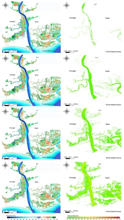
1.1 Classification of estuaries according to the primary process that shaped the underlying palaeovalley before the sedimentation during the Holocene, and based on the geomorphology and oceanographic characteristics, tides, and catchment hydrology (based on Hume and Herdendorf, 1988). ……….. 4 2.1 Study area and digital elevation model of the Guadiana estuary derived using bathymetric maps for year 2000 ……… 39 2.2 Relationship between the tidal inundation frequency and the depth below maximum spring high tide level for the present mean sea level and the IPCC (2007) sea level rise scenarios B1, A1B, and A1FI…..………. 45 2.3 Envelope of IPCC (2007) sea level rise scenario A1B (balanced use of fossil fuel). The 5% and 95 % curves are the lower and upper limits respectively of the A1B sea level rise scenario, and intermediate sea level rise curves represent intermediate percentile confidence limits (P) as denoted………. 47 2.4 Simulated morphological evolution: (i) depth below the maximum spring high-tide level relative to the mean sea level & (ii) net accretion of the Guadiana estuary by the end of the 21st
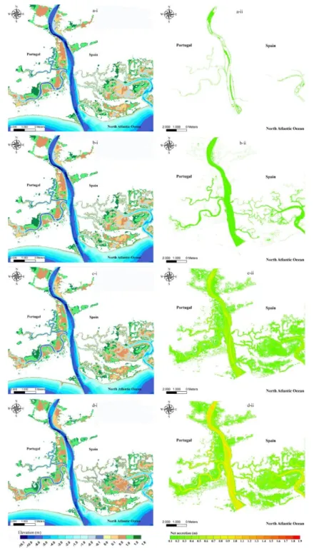
century for B1 sea-level rise scenario and for sedimentation scenarios: (a) HI (0.65 mm/y); (b) Min (1.3 mm/y); (c) Avg (2.1 mm/y); & (d) Max (3.9 mm/y) and the expansion of the intertidal zone area relative to the area in year 2000 is 6.1, 5.9, 5.4, & 4.1 km2, respectively………… 53 2.5 Simulated morphological evolution: (i) depth below the maximum spring high-tide level relative to the mean sea level and (ii) net accretion of the Guadiana estuary by the end of the 21st century for A1B sea-level rise scenario and for sedimentation scenarios: (a) HI (0.65 mm/yr); (b) Min (1.3 mm/yr); (c) Avg (3.7 mm/yr); and (d) Max (6.0 mm/yr) and the expansion of the intertidal zone area relative to in the area in year 2000 is 7.7, 7.6, 6.8, and 5.5 km2, respectively……….. 54
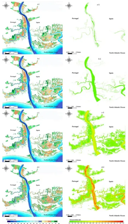
xxx
relative to the mean sea level and (ii) net accretion of the Guadiana estuary by the end of the 21st century for A1FI sea-level rise scenario and for sedimentation scenarios: (a) HI (0.65 mm/yr); (b) Min (1.3 mm/yr); (c) Avg (5.5 mm/yr); and (d) Max (9.7 mm/yr) and the expansion of the intertidal zone area relative to the area in year 2000 is 9.4, 9.3, 8.1, and 6.4 km2,
respectively……….. 55 2.7 Depth variations along the central longitudinal axis of the Guadiana estuary for sea level rise
scenarios B1 (0.38 m), A1B (0.48 m), and A1FI (0.59 m) and corresponding sedimentation scenarios (a, b, and c are the mean depth variation; and d, e, and f are the bed profile relative to present mean sea level)……… 56 2.8 Lateral movement of the 0 m contour of the Guadiana estuary in response to sea level rise scenarios (a) B1 0.38 m; (b) A1B 0.48 m; and (c) A1FI 0.59 m for each of four sedimentation rate scenarios (Max = sea level rise rate; Min = 1.3 mm/yr; Avg = 0.5(1.3 + sea level rise rate) mm/yr; and HI = 0.65 mm/yr, an approximation to account for the reduction in sediment supply due to human interventions such as dam construction). ………. 60 2.9 Morphological response of the Guadiana estuary to sea level rise and sedimentation scenarios:
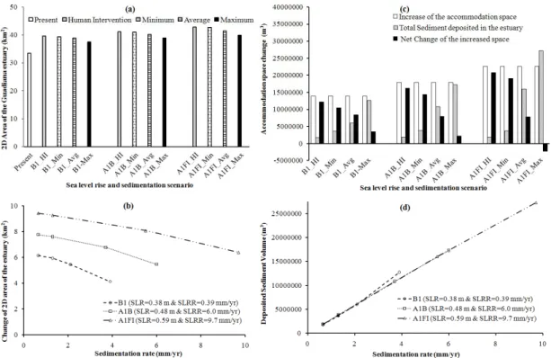
(a) Variation of the intertidal zone area; (b) Variation of the change of the intertidal zone area with sedimentation rate; c) Accommodation volume change of the estuary; d) Variation of sediment volume added with respect to change in sedimentation rate……….. 61
2.10 Cumulative sediment volume added into the Guadiana estuary for different percentile values of the A1B sea level rise scenario during the 21st Century for sedimentation rate scenarios: (a)
Max = sea level rise rate; (b) Min = 1.3 mm/yr; (c) Avg = 0.5(1.3 + sea level rise rate); (d) HI = 0.65 mm/yr)………... 64 2.11 Variation of cumulative sediment volume added with respect to sedimentation rate for the period 2010 to 2100 with a 10-year output time step and for percentile (P) values of 5, 15, 25, 35, 45, 50, 55, 65, 75, 85 and 95%. A percentile value is an expression of the uncertainty in the
xxxi
for the total data set belonging to each year………...65
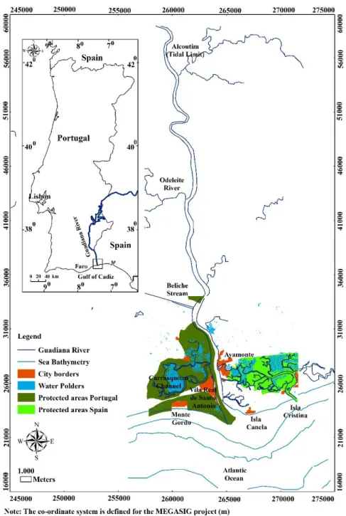
3.1 Location of the lower Guadiana Estuary……….. 84 3.2 Long-term net accretion rate coefficients as a function of depth of the Guadiana Estuary, where (a) and (b) represent two different distributions of sediment erosion coefficients () with depth, and (c) represents the distribution ofwith depth as in the case of (b) but with an additional proportion of net accretion observed at −0.75 m, which results in an equilibrium depth, compared with the observed equilibrium depth, of +2.0 m……….………. 95
3.3 Three-dimensional view of the reconstructed palaeovalley of the lower Guadiana Estuary at 11,500 cal. yr BP……….. 97 3.4 Comparison of palaeovalley simulation results corresponding to 0 cal. yr BP with the
present-day bathymetry derived from topo-bathymetric surveying in 2000 AD: (a) the palaeovalley of 11,500 cal. yr BP; (b) present-day bathymetry; (c), (d), (e), and (f) simulated present-day bathymetry under simulation runs 1, 2, 3, and 4, respectively……… 98
3.5 Three-dimensional sketch of sediment infilling over the Guadiana estuary palaeovalley from 11,500 cal. yr BP to the present (fourth simulation)……….. 101
3.6 Simulated curves of sediment infilling in the Guadiana estuary from 11,500 cal. yr BP to the present and comparison with actual present-day cross-sections……….……… 103
3.7 Lithostratigraphic sequences of boreholes a) CM-4 (Section 1); b) CM-3 (Section 3); and c) CM-1 (Section 5), showing sedimentary units and comparison of depths for ages obtained from radiocarbon (14C) analysis and model simulations (Adapted from Boski et al., 2002)…….. 104 3.8 Lithostratigraphic sequences of boreholes (a) CM-6 (Section 8); and (b) CM-5 (Section 9), showing sedimentary units and comparison of depths for ages obtained from radiocarbon (14C)
xxxii
equivalent modelled age for the same depths obtained from the simulation of the sediment infilling of the Guadiana estuary………. 108 3.10 Comparison of simulated and actual (observed) elevations for nine cross-sections along the Guadiana estuary for the present-day. The line y = x represents the ideal line for 100% accuracy between simulated and observed elevations………... 110 3.11 Sections of the Guadiana estuarine system for analysing errors on simulated bathymetries... 112 4.1. Location of the lower Guadiana estuary……….. 133 4.2 Time series used for forecasting morphological evolution in the Guadiana estuary during the 21st century: (a) sea level rise envelop of updated A1FI scenario; (b) corresponding decadal average sea level rise rate; and (c) the envelop of sedimentation scenario corresponding to A1FI sea level rise scenario and sediment supply reduction from fluvial sources……….. 135 4.3 Comparison of sediment types in the Guadiana estuary (a) Cluster Analysis of resemblance of the grannulometric distribution of marine sediment and fluvial sediment (b) the sediment types based on granulometric analysis of Morales et al., 2006……… 136
4.4 Comparison of spatial changes in the depth of the estuary below the maximum high tide level at present (2000) and at the end of each decade during the 21st century in response to the lower limit of A1FI sea level rise projections updated by Hunter (2010)………. 138 4.5 Comparison of spatial changes in the depth of the estuary below the maximum high tide level at present (2000) and at the end of each decade during the 21st century in response to the upper limit of A1FI sea level rise projections updated by Hunter (2010)………. 140
4.6 Comparison of spatial changes in net accretion of the estuary below the maximum high tide level at the end of each decade during the 21st century in response to the lower limit of A1FI
xxxiii
level at the end of each decade during the 21 century in response to upper limit of A1FI sea level rise projections updated by Hunter (2010)………. 144
4.8 Projected (a) decadal and (b) cumulative volume of sediment deposited on the estuary and its intertidal zone in response to the lower and upper limits of updated A1FI sea-level rise scenario during the 21st century……… 146
4.9 Decadal changes of area within depth classes (habitats) in the intertidal zone of the Guadiana estuary as a whole, above the mean sea level and below mean sea level during the 21st century
in response to: (i) lower limit and (ii) upper limit of A1FI sea level rise projections updated by Hunter (2010): (a) Changes in the Portuguese margin; (b) changes in the Spanish margin; and (c) Total changes………. 148
4.10 Decadal changes of the area within three depth classes (habitats) above the mean sea level of the Guadiana estuary during the 21st century in response to: (i) lower limit and (ii) upper limit of A1FI sea level rise projections updated by Hunter (2010): (a) Changes in the Portuguese margin; (b) changes in the Spanish margin; and (c) Total changes……… 149 4.11 Areas available at present for different habitat types likely to be in the estuarine system and their landward translation in the lower Guadiana Estuary in response to the lower and upper limits of A1FI Sea-level rise and sedimentation scenarios for the 21st century, if soil conditions are perfectly suitable for adaptation………..………….. 154 4.12 Comparison of morphological evolution using the direct application of behaviour-oriented Estuarine Sedimentation Model and modified ESM model based on hybrid rule-based theoretical framework of Prandle, (2006) and (2009)………..……….. 156 5.1 The Guadiana estuary and an aerial photograph of the lower estuary………... 168 5.2 River discharge of the Guadiana estuary as measured at the gauge station of Pulo do Lobo: (a) from 1946 to 2000 and (b) from 1990 to 2014 May……… 171
xxxiv
and pulse like large discharges with high fluctuations over a considerable period were averaged for simplicity in the Matlab script………... 177 5.4 Modelled tidal heights of the Guadiana estuary for a year in terms of 10 tidal constituents.. 180 5.5 Observed and simulated distributions of elevation change of the Guadiana estuary from 2000 to 2014. (a) Standard normal distribution and (b) normal distribution…… ………183 5.6 Sensitivity of bed friction coefficient (f) and power (n) of current velocity in the erosion rate function on determining the probability distribution of the elevation change of the Guadiana estuary from 2000 to 2014……….. 185 5.7 Sensitivity of estimated bed friction coefficient and power (n) of the current velocity of the erosion function on the average elevation change and corresponding standard deviation based on the simulated bathymetries of the Guadiana estuary for 2014……… 186 5.8 Observed bathymetries (z) and simulated bathymetries of year 2014 of the Guadiana estuary with respect to mean sea-level of the year 2000. (a) Observed z (2000); (b) observed z of (2014); (c) simulated z (n = 1.8 and empirically est. friction coefficients were reduced by 20%; (d) simulated z (n = 2 and empirically est. friction coefficients were not changed; (e) simulated z (n = 2.5 and empirically est. friction coefficients were increased by 50%; (f) simulated z (n = 3 and empirically est. friction coefficients were increased by 107%... 188 5.9 Observed and simulated elevation change of the Guadiana estuary from 2000 to 2014. (a) Observed Z; (b) simulated Z (n = 1.8 and empirically estimated friction coefficients were reduced by 20%; (c) simulated Z (n = 2 and empirically estimated friction coefficients were not changed; (d) simulated Z (n = 2.5 and empirically estimated friction coefficients were increased by 50%; (e) simulated Z (n = 3 and empirically estimated friction coefficients were increased by 107%... 189
xxxv
changes in the standard deviation for four cases of (1) n = 1.8 & friction coefficients were reduced by 20%; (2) n = 2 & no change in friction coefficients; (3) n = 2.5 & friction coefficients were increased by 50%; (4) n = 3 & friction coefficients were increased by 107%... 192 5.11 Sensitivity of sea-level rise rate on the elevation change of the estuary bed. (a) Average elevation change with sea-level rise rate, (b) standard deviation with sea-level rise rate and (c) additional relative net accretion rate with sea-level rise rate……….. 194 5.12 Observed and simulated normal distribution of the elevation change in the Guadiana estuary from 2000 to 2014 for four cases of (1) n = 1.8 and friction coefficients were reduced by 20%; (2) n = 2 and no change in friction coefficients; (3) n = 2.5 and friction coefficients were increased by 50%; (4) n = 3 and friction coefficients were increased by 107%... 195 7.1 The observed and modelled flow of the Guadiana River from 2000 to 2014 May. (a)
Comparison of the observed river discharge with the modelled discharge (b) Comparison of the observed river discharge with modelled discharge but the coefficients of the trigonometric function (base flow) were increased by 1.5; & (c) the same was increased by 2……… 237 7.2 Representative sedimentation rate functions for modelled river discharge, which was approximated to the observed river discharge of the Guadiana River from 2000 to 2014 and modelled river discharge for the same period but the coefficients of the trigonometric function (base flow) were increased by 1.5 and 2………. 238 7.3 Sea-level rise projections: (a) The upper limit projection of A1FI (Intensive use of fossil fuel) sea-level rise scenario based on the IPCC, 2007 report but updated including the effect of ice sheet melting (Hunter, 2010); and (b) Corresponding sea-level rise rate variations……….. 239 7.4 Bathymetry of the Guadiana estuary (a) observed in 2000 and the simulated bathymetries for (b) 2020, (c) 2050, (d) 2070 and (e) 2100, in response to the A1FI sea-level rise scenario and the modelled river discharge, which equivalent to the observed river discharge pattern at the Pulo do Lobo Guage station……… 241
xxxvi
level rise scenario and sedimentation scenario based on river discharge (a) app. equivalent to the observed river discharge pattern from 2000 to 2014 May; (b) the base flow of the modelled river discharge in the case a was increased by factor 1.5; and (c) by a factor 2………. 244 7.6 Change of elevation of the Guadiana estuary at the end of year (a) 2020; (b) 2050; and (c) 2100 in response to sea-level rise by 79 cm (The upper limit of the A1FI scenario) and sedimentation scenario based on river discharge (i) approximately equivalent to the observed river discharge pattern from 2000 to 2014 May; (ii) the base flow of the modelled river discharge in the case a was increased by factor 1.5; and (iii) by a factor 2………. 245 7.7 Decadal volume of sediment erosion, accreted and net erosion from the lower Guadiana estuary due to A1FI sea-level rise scenario and sedimentation scenario based on river discharge (a) approximately equivalent to the observed river discharge pattern from 2000 to 2014 May; (b) the base flow of the modelled river discharge in the case a was increased by factor 1.5; and (c) by a factor 2……… 247
xxxvii
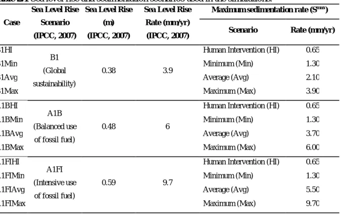
2.1 Sea level rise and sedimentation scenarios used in the simulations……….. 48 3.1 Input data used to model Holocene sediment infilling in the Guadiana Estuary……….. 94
3.2: Summary information for 14C age determinations showing conventional age, 13C‰, 2 range and indicative ages used in the text and Fig. 3.6, 3.7, 3.8 and 3.9……… 102 3.3 Comparison of root mean square errors on simulated water depths and corresponding actual depths and average errors on simulated accretion heights relative to those of actual accretion heights of the Guadiana estuarine system from 11,500 cal yr BP to the present……… 115
4.1 Predicted translation of area of the likely habitat types in the intertidal zone of the Portuguese margin in response to lower and upper limit scenarios of sea level rise and sedimentation by the year 2100, compared to their existing area by 2000……… 151 4.2 Predicted translation of area of the likely habitat types in the intertidal zone of the Spanish
margin in response to lower and upper limit scenarios of sea level rise and sedimentation by the year 2100, compared to their existing area by 2000………. 152 5.1 Tidal constituents used for determining the tidal heights in the model (Pinto, 2003)………. 180 6.1 Corrected average denudation rate of the Guadiana river basin by applying assumed sediment retention factor due to dams……… 220 7.1 Coefficients that used to change the base flow of the Guadiana river discharge, which is approximated as a combination of sinusoidal and cosine functions……… 236 7.2 Predicted translation of area of the likely habitat types in the intertidal zone of the Guadiana estuary in response to upper limit scenarios of sea level rise and sedimentation scenarios by the year 2100, compared to their existing area by 2000……… 242
1
Chapter 1
2
1.1 GENERAL INTRODUCTION
1.1.1 WHAT IS AN ESTUARY AND HOW IT IS FORMED AND EVOLVE?
An estuary is the seaward portion of a drowned river valley (Dalrymple et al., 1992) and it is a semi-enclosed transitional water body (Potter et al., 2010) that extends from landward tidal limits to the seaward limit of coastal influence (Cameron and Pritchard, 1963; Nichols and Biggs, 1985). Thus, in chemical terms the salinity range in an estuary extends from 0.5 to 30-35 ‰ (Pritchard (1967). River valleys incised due to erosion in response to a fall in sea-level during low stands (Fagherazzi et al., 2004). Then they were drowned forming the present morphology of estuaries by the subsequent postglacial sea-level rise during the Holocene (Roy et al., 1994). Estuaries have since infilled with marine and fluvial sediment to varying degrees depending on the global forcing like sea-level rise rate (Bridge, 2003) and local controls including wave climate, the availability of riverine and coastal sediment, and the river and tidal hydrodynamics (Wright and Coleman, 1973).
In meso-tidal regimes (tidal range 2 - 4m), fluvial discharge controls the geomorphologic evolution of the estuary (Wolanski, 2006). However the observed high variability in valley morphologies may be due to other controlling factors including hydrodynamics, sediment supply, geomorphology, climate and human activities (Chaumillon
3
et al., 2011). The life span of an estuary extends over a millennial time scale passing through several stages of life from youth to maturity and old or terminal age (Roy, 1984; Roy, 1994; Roy et al., 2001). According to Wolanski, 2006, at the first stage the river valleys are flooded due to sea-level rise and during the second stage, tidal inundation fosters the growth of salinity resisting vegetation and finally, during the terminal stage, freshwater vegetation will dominate the habitat as the plains become higher in elevation than high tide limits due to various forms sedimentation.
1.1.2 CLASSIFICATION OF ESTUARINE SYSTEMS
In terms of management and modelling perspectives, setting the right typology of estuaries is important because it defines the dominant processes in the long term evolution of the estuarine morphology. According to geomorphological features of estuaries, Pritchard, (1967) proposed a four type classification: (1) drowned river valleys, (2) fjord type estuaries, (3) bar-built estuaries and (4) estuaries produced by tectonic processes. Based on geomorphology and topography, Davidson et al., (1991) classified estuaries into nine categories: (i) fjord, (ii) fjard, (iii) ria, (iv) coastal plain, (v) bar built, (vi) complex, (vii) barrier beach, (viii) linear shore and (ix) embayment. According to the primary process that shaped the underlying palaeovalley before the sedimentation during the Holocene, Hume and Herdendorf (1988) divided estuaries in to five classes with sixteen sub-classes based on the geomorphology and oceanographic characteristics of the estuary, and catchment hydrology (Fig. 1.1). Hume et al., (2007) presented a new classification of estuaries based on a hierarchical view of the abiotic components that define estuarine environments. Accordingly, estuaries are grouped into four levels: (1) global scale variation based on differences in climatic and oceanic processes (Solar radiation, heating and cooling, precipitation, evaporation), which are discriminated by the factors: latitude, oceanic basins and large landmasses; (2) variation in
4
estuary hydrodynamic processes (mixing, circulation, stratification, sedimentation, and flushing), which are discriminated by estuary basin morphometry, river and oceanic forcing; (3) variation among estuaries that are due to catchment processes (Supply of fresh water, sediment and water chemistry constituents), which are discriminated by catchment geology and catchment land cover; and (4) variation among estuaries that are due to local hydrodynamic processes Sediment deposition and erosion, which are discriminated by ocean swell, tidal currents, wind waves and depth.
Figure 1.1 Classification of estuaries according to the primary process that shaped the
underlying palaeovalley before the sedimentation during the Holocene, and based on the geomorphology and oceanographic characteristics, tides, and catchment hydrology (based on Hume and Herdendorf, 1988).
5
It was recognized that the tidal range (Dyer, 1996) increases upstream with the convergence of the estuarine margins while friction reduces the tidal range. Thus, according to the dominance of the friction and convergence over the tidal range, estuaries also can be classified as hypersynchronous, synchronous and hyposynchronous (Nichols and Biggs, 1985). If the convergence forcing exceeds friction, they are called hypersynchronous estuaries, in which tidal range and current increase towards the head of these funnel shaped estuaries and in the riverine section, tidal range reduces as the friction increases (Dyer, 1996). The opposite is true for hyposynchronous estuaries. In synchronous estuaries, the effect of friction and convergence of margins on tidal range is equal and the sea surface slope due to axial gradient in phase of tidal elevation significantly exceeds the gradient from changes in tidal amplitude (Prandle, 2009).
In the context of facies distribution of estuaries, Dalrymple et al., (1992) grouped them according to the dominance of tides and waves. Accordingly, in a wave dominated estuary, its mouth experiences high wave energy and the sediment eroded in the adjacent coastline will be deposited to form a subaerial barrier/spit or submerged bars. As the mouth is constricted with increased deposition, currents will increase so as to have balance in sediment deposition and erosion (Dyer, 1996). In tide dominated estuaries, tidal currents play the dominant role in transporting the fluvial sediments, resulting in significant upstream transport of bedload sediment (Wells, 1995). In such estuaries, mouth area will be flanked by sandbanks aligned with the dominant direction of the current flow (Dyer, 1996). Interestingly, Chaumillon et al., (2011) identified a mixed system which can be classified as neither tide nor wave dominated. However, they cannot be defined solely according to the magnitudes of tidal range (Wells, 1995). If the rising-tide time is shorter than the falling-tide time, such estuaries are flood-dominant while the opposite is true for ebb flood-dominant systems (Wang et al., 2002). Chaumillon
6
et al., (2011) defined a schematic representative cross sections showing the variability of French valley fills related to their energetic and morphologic classification.
On the basis of vertical structure of salinity, estuaries can be further classified as salt wedge, strongly stratified (salt-wedge or Fjord type), weakly stratified (partially mixed) or vertically mixed (laterally homogeneous or inhomogeneous) (Cameron and Pritchard, 1963; Dyer, 1996). The estuarine circulation will be controlled by the balance between the pressure gradient induced by the outer estuary surface slope, the baroclinic pressure gradient due to the along-estuary salinity gradient, and the stress associated with the estuarine circulation (Geyer et al., 2000). Therefore, this classification considers the balance between buoyancy forcing from river discharge and mixing from tidal forcing, which determines the volume of oceanic water entering the estuary during each tidal cycle (Valle-Levinson, 2010). In vertically stratified estuaries, there would be no mixing of salt and freshwater (Dyer, 1996), which can be observed in large river discharge combined with weak tidal forcing particularly during the flood tide (Valle-Levinson, 2010). In partially mixed estuaries, there is a significant vertical density gradient (Fischer, et al., 1979) resulting from moderate to strong tidal forcing and weak to moderate river discharge (Valle-Levinson, 2010). In a vertically homogeneous estuary, there is sufficient mixing so that the salt-water and fresh water interface disappears at high tidal current velocities (Biggs, 2012) and weak river discharge (Dyer, 1996). Consequently, mean salinity profiles in mixed estuaries are practically uniform and mean flows are unidirectional with depth (Valle-Levinson, 2010).
However, it is important to note that defining a mutually exclusive classes of estuaries may not be practical, given that some estuaries may belong to more than one class as there is a range of properties and processes (Wells, 1995). Many estuarine systems may change from one class to another in subsequent tidal cycles, or from month to month, or from season to season (dry or wet), or from one location to another within the same estuary (Valle-Levinson, 2010).