Adsorption of colloidal particles on mobile rafts

(1)

UNIVERSIDADE DE LISBOA

FACULDADE DE CIÊNCIAS

DEPARTAMENTO DE FÍSICA

Adsorption of colloidal particles on mobile rafts

Diogo Estêvão Pereira Pinto

Mestrado em Física

Física da Matéria Condensada e Nano-materiais

Dissertação orientada por:

Professor Doutor Nuno Araújo

(2)

(3)

Acknowledgements

I would like to thank Nuno Araújo and Margarida Telo da Gama, for introducing me to the topic of physics far-from-equilibrium, for which I grew very found off, and also for their hard work, persistence and for standing by my side through this whole process. I would also like to thank Cristóvão Dias, André Nunes and Francisco Braz for their helpful input. Finally, I would like to give a special thanks to my parents and Ana Sofia for always being present. This objective was only made possible because I have a great group of people supporting me.

I would like to acknowledge the financial support from the Portuguese Foundation for Science and Technology (FCT) under Contract no. IF/00255/2013.

(4)

(5)

Abstract

Colloidal particles trapped at oil-water interfaces interact through long-range capillary forces resulting from the deformation of the interface. As a result, kinetically trapped structures are obtained and expected quasi-2D thermodynamic phases are rarely obtained. A scheme was recently proposed to avoid such strong particle-particle interactions and to obtain a fully ergodic quasi-2D colloidal dynamics. The idea is to adsorb DNA-coated colloidal particles on complementary DNA patches that are diffusing on the surface of the oil droplets. Here, we develop a theoretical model that replicates the relevant physical properties of the experimental system.

We perform an extensive numerical study of the model using a kinetic Monte Carlo algorithm. We find that the coverage, for an earlier stage of the evolution, does not depend strongly on the diffusion coefficient. However, as time evolves differences become evident. We also observe that as the system reaches jamming, the number of parameters that describe the coverage evolution can be reduced. We supplement this study with an analytical approach using a mean-field approximation. With it, we are able to reach closed form equations that describe the time evolution of the density of adsorbed particles and patches, and show that the numerical data follows the same functional dependency. We also show that our results are able to reproduce, qualitatively, what is seen in the experiments.

Finally, we use a one-dimensional continuum model to study numerically the irreversible ad-sorption of particles on the patches, with the focus on the possible configurations created due to the random sequential adsorption. Here, we study how the number of adsorbed particles on the patch de-pends on the ratio between their respective sizes. We support this study with an analytical approach, which enumerates the possible configurations of the model for certain patch sizes. We show that the analytical results are in very good agreement with the numerical ones.

KEYWORDS:

(6)

(7)

Resumo

Nesta tese é apresentado um estudo da adsorção de part´ıculas coloidais cobertas com ADN, em gotas de óleo funcionalizadas com o ADN complementar. Este sistema visa reduzir a deformação da superf´ıcie da gota causada pela adsorção das part´ıculas coloidais. Usando este método, é poss´ıvel evitar o aparecimento de forças capilares de longo alcance entre part´ıculas coloidais adsorvidas na interface, que leva à formação de estruturas presas pela cinética. Assim, é poss´ıvel desenvolver um sistema em que a dinâmica das part´ıculas após a adsorção é ergódica, e as estruturas termodinâmicas mais estáveis estão acess´ıveis pela cinética.

O sistema f´ısico consiste em gotas de óleo submersas numa solução aquosa, estabilizadas por moléculas SDS. Na sua superf´ıcie são adsorvidas cadeias de pol´ımeros PLL-PEG-bio, que podem di-fundir ao longo da superf´ıcie da gota. Depois, cadeias únicas de ADN são introduzidas aos pol´ımeros, de modo a formar patches de ADN. Cobrindo as part´ıculas coloidais com as cadeias de ADN com-plementares, é poss´ıvel introduzir uma interação seletiva entre as part´ıculas e a superf´ıcie da gota. Usando este método, é poss´ıvel mostrar que a deformação da superf´ıcie da gota se torna desprezável. A adsorção das part´ıculas na superf´ıcie da gota, apesar de muito forte, pode ser revertida aumentando a temperatura. Experimentalmente, observa-se que a cobertura da gota não só depende da dinâmica na sua superf´ıcie mas também da concentração de part´ıculas coloidais em solução.

Para estudar este sistema, foi desenvolvido um modelo teórico que tenta capturar as suas pro-priedades f´ısicas mais relevantes. Este consiste num substrato, modelado como uma rede, com um certo tamanho em unidades de s´ıtios de rede, onde os patches difundem, com um dado coeficiente de difusão D. As part´ıculas tentam adsorver no substrato com um fluxo F . Estas só podem adsorver em patchesque estejam livres, e, tanto a interação part´ıcula-part´ıcula como a interação patch-patch são considerada como de volume exclu´ıdo. Depois de uma part´ıcula adsorver se ainda possuir espaço não ocupado por baixo da mesma, outro patch que esteja a difundir pode encontrá-la e agregar-se a ela. Usando este modelo é poss´ıvel estudar a adsorção irrevers´ıvel das part´ıculas coloidais nos patches, e ver como a cobertura da gota depende dos parâmetros do sistema.

Uma das nossas abordagens a este problema foi numérica. Para seguir a dinâmica do sistema usámos o método de Monte Carlo cinético. Como sabemos todos os processos que podem acontecer e as respetivas taxas, é poss´ıvel gerar um catálogo de processos, e assim formular um algoritmo sem rejeições. Este é bastante útil, pois possibilita a exploração de escalas de tempo mais longas de uma forma bastante eficiente quando comparado com outros método como Dinâmica Molecular. Este método faz uso de um relógio f´ısico e tem em conta toda a sequência de eventos até chegar à configuração final (ao contrário de MC standard), fornecendo informações fundamentais para estudar a dinâmica.

Nós estudámos este modelo em uma e duas dimensões. Em ambas os patches são modelados como monómeros, enquanto que as part´ıculas para 1D são d´ımeros e em 2D quadrados com largura igual a dois em unidades de s´ıtios de rede. O nosso foco foi direcionado para a evolução temporal da

(8)

cobertura, onde observámos que a mesma aumenta monotonicamente ao longo do tempo. Também observamos que, para fluxos altos, a cobertura no jamming tende para o valor assimptótico de uma part´ıcula por patch. Isto deve-se ao facto de que quando F aumenta os patches vão ter menos tempo para se agregarem entre adsorções sucessivas. Também observámos que diminui com o aumento do coeficiente de difusão, dado que este aumenta a probabilidade de patches se agregarem, o que diminui o número de patches livres em que as part´ıculas podem adsorver.

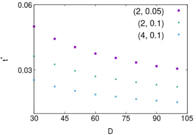
Para tempos baixos, verifica-se que a cobertura do sistema tem uma dependência desprezável no coeficiente de difusão dos patches. Esta observação vem do facto de as curvas da cobertura em função do tempo, para diferentes coeficientes de difusão, quase se sobreporem à de D = 0. Assim, é poss´ıvel definir um tempo, t∗, que mede como as curvas da cobertura para diferentes D se desviam da de D = 0. É poss´ıvel observar que t∗ decresce com D, dado que quanto maior D mais rápido os patches encontram outras part´ıculas adsorvidas, produzindo um efeito na cobertura do sistema. Para além disso, t∗também decresce com n0(definido como a densidade inicial de patches), porque

quanto maior n0, menor a distância t´ıpica entre patches, o que promove a sua agregação. t∗também

decresce com F , dado que este aumenta o número de tentativas de adsorção de part´ıculas, levando a uma mais rápida cobertura do sistema. Estes resultados foram observados tanto para uma dimensão como para duas.

O passo seguinte foi estudar o estado de jamming. Aqui observámos que o número de parâmetros relevantes para o sistema quando ele chega ao jamming é reduzido. Enquanto que durante a dinâmica inicial tanto F como D são parâmetros relevantes, ao chegar ao jamming o parâmetro relevante passa a ser a razão F/D. Também observámos que a cobertura no jamming cresce monotonicamente com F/D, devido à competição entre as duas escalas de tempo envolventes: o tempo browniano caracter´ıstico da difusão dos patches e o tempo de chegada das part´ıculas à interface. Sendo assim, quando F/D aumenta mais part´ıculas vão conseguir adsorver, dado que vai ser menos provável que os patches consigam encontrar part´ıculas para agregar entre adsorções sucessivas. Este resultado foi observado para uma e duas dimensões. Este resultado vem ao encontro do que foi observado experimentalmente, onde se vê que aumentar a concentração de part´ıculas coloidais na solução (que corresponde a um aumento de F neste modelo), leva a um aumento da cobertura da gota.

Também abordámos o problema analiticamente usando uma aproximação de campo médio, de modo a estudar a evolução temporal da densidade de part´ıculas adsorvidas (cobertura) e de patches livres. Tendo em conta apenas os processos de adsorção de part´ıculas e agregação de patches, e de-sprezando as correlações espaciais, é poss´ıvel chegar a duas equações exatas para o nosso problema. Tirando o limite assimptótico (t → ∞) das equações, é poss´ıvel observar que o número de parâmetros necessários para descrever a densidade de part´ıculas adsorvidas (que é igual à cobertura) é reduzido, passando de F e D, para F/D. Também estudámos o comportamento inicial das funções expandindo-as em torno de t = 0, onde observámos que os primeiros dois termos da expansão não dependem de D, e este parâmetro só surge no termo de terceira ordem. Por isso, enquanto o termo de terceira ordem é desprezável, a densidade de part´ıculas adsorvidas evolui aproximadamente como observado para D = 0. Comparando os resultados anal´ıticos com os da simulação usando o modelo de rede é poss´ıvel observar as mesmas dependências funcionais nos parâmetros, tanto para uma dimensão como para duas.

O último estudo que esta tese foca é a descrição do sistema no cont´ınuo. Para este estudo, propomos um modelo em que as part´ıculas são modeladas como segmentos de um certo tamanho e o patch também como um segmento com de tamanho diferente. As únicas interações tidas em conta são as de volume exclu´ıdo entre part´ıculas. Para estudar este modelo numericamente, um algoritmo

(9)

foi desenvolvido que se foca na localização de intervalos abertos onde part´ıculas podem adsorver no patch sem sobrepor outras. Assim é poss´ıvel formular um algoritmo eficiente sem rejeições. Este estudo tem como objetivo compreender como a cobertura do patch depende da razão entre os tamanhos das part´ıculas e do patch (AR). Observamos que para AR > 1, o número de part´ıculas adsorvidas aumenta monotonicamente com o AR. No entanto para 0 < AR < 1, dado que uma única part´ıcula pode cobrir completamente o patch, a dependência em AR é diferente.

Também desenvolvemos uma abordagem anal´ıtica que se foca na enumeração de todas as poss´ıveis configurações . Aqui apresentámos os cálculos para 0 < AR < 1 e 1 < AR < 2. Comparando com os obtidos numericamente observámos que ambos estão em excelente acordo.

(10)

(11)

List of Figures

2.1 Representation of the various stages of the sample preparation . . . 4 2.2 Representation of the rules of the model . . . 6 3.1 Coverage as a function of time, for dimer adsorption on a one-dimensional lattice . . 14 3.2 Coverage as a function of time, for monomer adsorption on a two-dimensional lattice 15 4.1 One-dimensional lattice model for dimers adsorbing on monomers . . . 17 4.2 Coverage as a function of time, for the one-dimensional lattice . . . 18 4.3 Coverage as a function of time, for n0 = 0.03 (a) and n0= 0.1 but higher values of

the diffusion coefficient (b), for the one-dimensional lattice . . . 18 4.4 t∗as a function of D, for different sets of parameters (F, n0), for the one-dimensional

lattice . . . 19 4.5 Coverage as a function of time for different F and D, for the one-dimensional lattice 19 4.6 Jamming coverage as a function of a) F for D = 1, 2, 3, b) D for F = 2, 5, 10, and

c) the ratio F/D, for the one-dimensional lattice model . . . 20 4.7 Jamming Coverage as a function of F/D for different n0, for the one-dimensional

lattice . . . 21 4.8 Jamming coverage as a function of the ratio F/D (a), and coverage as a function of

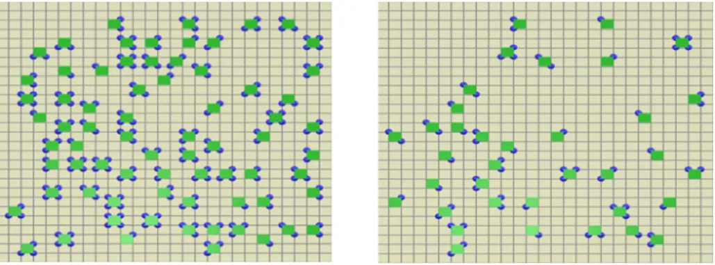
time (b), for different system sizes . . . 21 4.9 Snapshots of the simulations for two different n0 . . . 22

4.10 Coverage as a function of time, for two-dimensions . . . 23 4.11 t∗as a function of D, for different set of parameters (F, n0), for the two-dimensional

lattice . . . 23 4.12 Coverage as a function of time for different F and D, for the two-dimensional lattice 24 4.13 Jamming coverage as a function of the ratio F/D, for the two-dimensional lattice . . 25 4.14 Jamming coverage as a function of F/D for different n0, for the one-dimensional

lattice . . . 25 4.15 Jamming coverage as a function of the ratio F/D (a), and coverage as a function of

time (b), for different system sizes . . . 26 4.16 Plot of Eq 4.8 for different D . . . 28 4.17 t∗, as defined in Eq. 4.2, as a function of (F2n2₀D)−1/3. Comparison between the

analytical result and the numerical data for the one- and two-dimensional simulations 29 4.18 Coverage as a function of time. Comparison between the analytical result and the

numerical data for the one- and two-dimensional lattices . . . 29 4.19 Jamming coverage as a function of the ratio F/D. Comparison between the

(14)

List of Figures

5.1 One-dimensional continuum model for particle adsorption on a patch . . . 32 5.2 Average number of particles adsorbed as a function of the aspect ratio for the

one-dimensional continuum model . . . 34 5.3 Probability of adsorbing n = 1, 2, 3, 4, 5 particles on the patch as a function of the

aspect ratio for the one-dimensional continuum model . . . 34 5.4 Schematic of the possible configurations when adsorbing only two particles with

0 < AR < 1, in the one-dimensional continuum model . . . 35 5.5 Average number of particles adsorbed on a patch with linear size in the interval 0 <

r < 1, in the one-dimensional continuum model . . . 37 5.6 Probability of adsorbing n = 1, 2 particles on a patch with linear size in the interval

0 < r < 1, in the one-dimensional continuum model . . . 38 5.7 Schematic of the possible configurations when adsorbing only two particles with

1 < AR < 2, case A, in the one-dimensional continuum model . . . 38 5.8 Schematic of the possible configurations when adsorbing only two particles with

1 < AR < 2, case C, in the one-dimensional continuum model . . . 39 5.9 Schematic of the possible configurations when adsorbing only two particles with

1 < AR < 2, case D, in the one-dimensional continuum model . . . 39 5.10 Average number of particles adsorbed on a patch with linear size in the interval 1 <

r < 2, in the one-dimensional continuum model . . . 40 5.11 Probability of adsorbing n = 2, 3 particles on a patch with linear size on the interval

(15)

Acronyms

SDS Sodium Dodecyl Sulfate

PLL-PEG-bio Polylysine-g-Polyethyleneglycol-biotin RSA Random Sequential Adsorption

kMC kinetic Monte Carlo

BD Brownian Dynamics

MC Monte Carlo

RNG Random Number Generator

(16)

(17)

Chapter 1

Introduction

With the sustained development of new technologies, experiments have been able to reach smaller and smaller scales, down to the nano-scale. This development provides the tools to synthesize new devices with enhanced physical properties and to study systematically previously observed phenom-ena. For example, it was possible to uncover the mechanism responsible for the change of skin color of certain reptiles, like chameleons. Today we know that the color change is related to changes in the structure of the skin (structural color) and not to the chemical composition (pigments), as initially hypothesized [1, 2]. What was observed is that they rapidly change color by actively deforming an array of small crystals, with typical sizes of the order of the wavelength of light, on the surface of their skin, which in turn changes the wavelength of the reflected/diffracted light.

The physical properties of a material depend strongly on the spatial arrangement of their indi-vidual constituents. Thus, there has been a sustained interest on developing experimental strategies to synthesize materials with a fine control over their structure. Colloidal particles are very popular for this goal [3–7], mostly because currently available techniques allow us to synthesize them in large amounts with very good control over their shape and size [8, 9]. Furthermore, they are ideal building blocks for optical materials since they have a typical size of the order of the wavelength of light. One method that can be used to control the structure is self-assembly, which designates the process through which larger structures are spontaneously formed from their smaller constituents, by taking advantage of the properties present in the constituents themselves and without the application of external perturbations. This method has received significant attention from the scientific commu-nity [10–15], since on one hand, it is less expensive than other methods to produce materials at small scales, and, on the other, it is easier to scale up and achieve massive production.

One example of a challenge in self-assembly is the formation of ordered, quasi-two-dimensional patterns of many distinct colloidal or nano particles. One promising route is to use substrates as a support for the growth of planar structures [16–20]. For that, the substrate must be smooth at the colloidal scale (micron) and the colloidal particles need to be able to bind independently and irreversibly to the surface. Another important detail is that the adsorbed particles should be mobile enough so that the most stable (thermodynamic) structures are kinetically accessible. For strong enough particle-substrate interactions, the mobility of particles after adsorption is compromised, hindering an ergodic dynamics of particles on the substrate. Under such conditions, the obtained structures are strongly dependent on the kinetics of adsorption on the substrate [3].

Methods based on the adsorption on solid substrates have been considered to synthesize mate-rials for a wide range of applications, like quantum dots, photonic crystals, sensors, heterogeneous catalysts and microarrays [21–24]. For example, by using pre-patterned substrates it is possible

(18)

Chapter 1. Introduction

to control the dynamics of the adsorbed particles and induce local order in the first adsorbed lay-ers [17, 21, 25, 26]. A problem with this kind of approach is that the strength of particle-substrate interaction is either very strong, and mobility after adsorption is compromised, or too weak and one cannot guarantee irreversible binding to the substrate, compromising the success of the strategy.

One alternative is the adsorption of colloidal particles on liquid-liquid interfaces, such as an oil droplet in water, forming a Pickering Emulsion [27, 28]. Using thermodynamic arguments, it is possible to show that the colloidal particles on the interface are energetically favored, as the surface energy is reduced by several kBT [18, 27, 28]. However, as the particles will deform the interface,

to guarantee a constant contact angle, long-range capillary inter-particle forces will emerge [29, 30], which promote a strong particle-particle attraction, leading to the formation of kinetically arrested structures that are significantly different from the thermodynamic ones.

To avoid strong capillary interactions and achieve an ergodic dynamics of the colloidal particles, we have proposed a method based on DNA mediated interactions [31]. By covering the surface of the oil droplet with single strands of DNA and the colloidal particles with the complementary ones, it is possible to create a selective particle/substrate interaction. A key aspect of this system is that the DNA strands are mobile and therefore the particles, after adsorbing, will be able to move without significantly deforming the interface. Using this method, the adsorption of colloidal particles to the interface is still very strong though reversible, since above a certain temperature the two DNA strands in the double helix structure unbind from each other.

Experimentally, using this strategy, it is observed that the coverage of the oil droplets is not only dependent on the dynamics on its surface but it depends also on the bulk concentration of colloidal particles in solution [31]. Given the irreversible nature of the bond formation with the substrate (for fixed temperatures), we are dealing with a system out of equilibrium and so the connection be-tween these quantities is not trivial and should be significantly different from the classical Langmuir (reversible) dynamics. Unfortunately, it is hard to explore a large range of the parameter space in experiments due to resource (materials and time) constraints. Also, to study the dynamics it is neces-sary to use individual particle tracking methods which can be quite complex to implement, specially in the bulk. Thus, we developed a theoretical approach to shed light on the dynamics of this system. Combining analytic calculations with simulations, it is possible to explore systematically a wider region of the parameter space as well as to follow the dynamics, and therefore shed light on the experimental results and guide new experiments.

Numerically, we employed a kinetic Monte Carlo method to simulate the adsorption of the col-loidal particles on the surface of the oil droplet. By relating the bulk concentration of colcol-loidal parti-cles to the rate at which they attempt adsorption on the substrate, we are able to develop a stochastic model that enables us to analyze the kinetics of adsorption. In this way, it is possible to explore how the coverage of the surface evolves in time and how it depends on the dynamical parameters of the model. The behavior of the model is discussed for one- and two-dimensional lattices. We also discuss a continuum limit focused on the adsorption of particles on a single DNA patch, with the goal of understanding the different configurations that are possible to create and how they depend on the size of the particles and of the patch.

The thesis is organized as follows: In Chapter 2, the physical system and the theoretical model is defined. Chapter 3 includes details about the simulation techniques used and some code validation examples. In Chapter 4, we report on the kinetics of adsorption on a lattice. In Chapter 5, we discuss the continuum limit of the model. In Chapter 6, some concluding remarks are drawn.

(19)

Chapter 2

The Physical System

2.1 DNA-functionalized colloidal particles and oil droplet

Many systems have been explored where DNA functionalized fluid surfaces have been used. For example, functionalizing vesicles or fluid membranes with single-stranded DNA [32, 33], or functionalizing fluid membranes enveloping hard spherical colloidal particles [34]. The motivation for using fluid substrates is to ensure that the grafted single strand DNA can diffuse on its surface without significantly deforming it, which leads to fully ergodic colloidal dynamics after adsorption. With this, it is possible to use the fluid surface as substrate for the adsorption of colloidal particles functionalized with the complementary DNA, which then self-assemble into ordered or amorphous structures depending on the experimental conditions [35–39].

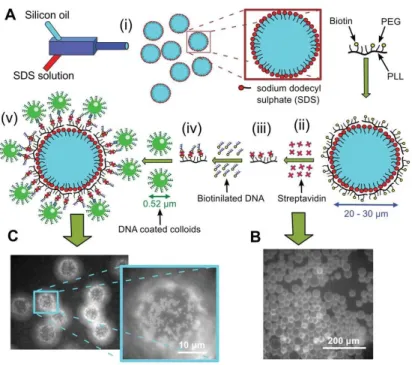
Our approach (Fig. 2.1) begins with the production of oil droplets with a typical diameter of 20 to 30 µm, stabilized by sodium dodecyl sulfate (SDS), which are molecules with a hydrophilic tail and hydrophobic head group. Thus, after they adsorb on the interface of the oil droplet they form a micelle which will be used as substrate for the DNA patches. To it, a comb-like poly-electrolyte (PLL-PEG-bio) is adsorbed. As illustrated in Fig. 2.1, the positively charged poly-lysine backbone adsorbs in a flat manner onto the negatively charged SDS head-groups that are exposed to the oil-water interface. Half of the roughly 40 PEG chains per PLL backbone carry a biotin group, which are functionalized with streptavidin from solution. Finally, single strands of DNA are brought onto the oil droplets surface via the streptavidin. Thus, it is possible to create small flat patches of PLL molecules (DNA patches) that diffuse freely with their DNA on the droplets surface. When 0.57 µm large polystyrene particles with the complementary single strand DNA, are added to the solution they anchor reversibly to the surface via DNA hybridization. An important aspect of this method is that since the colloidal particles are larger than the DNA patches, after one adsorbs, the DNA patches that are diffusing can find this adsorbed particle and accumulate bellow it forming ‘rafts’, with complementary functionalization. After the adsorption process, the rafts formed bellow the particles are still able to diffuse with the particle attached.

There are three important experimental observations: first, the adsorption of the colloidal parti-cles on the interface is mediated by DNA; second, this hybridization between colloidal partiparti-cles and complementary DNA on the surface of the oil droplets is thermally reversible; third, the adsorbed colloidal particles diffuse on the surface of the oil droplet [31].

With this method it is also possible to show that one can control the surface coverage of oil droplets by colloidal particles, by exploiting the fact that during slow adsorption, compositional arrest takes place well before structural arrest occurs, as the diffusion of the rafts is almost negligible

(20)

Chapter 2. The Physical System

within the time scale of colloid adsorption. Also, the diffusion of the rafts is, at least, one order of magnitude smaller than the one of the patches. Thus, it is possible to separate the theoretical analysis into two different time scales. A fast one, where compositional arrest occurs, corresponding to the adsorption of particles to the surface of the oil droplets, and a slow one that corresponds to the structural arrest and represents the aggregation of the colloidal particles. In this thesis, we will focus on the first one. For details about the second, please refer to [31].

Another relevant observation from the experimental data was that the coverage of the oil droplets by colloidal particles not only depended on the dynamics on its surface but also on the bulk concen-tration of colloidal particles in solution. The motivation for the work in this thesis comes from this experimental observation, and on the following chapters our results will be presented with the goal of studying the fast regime of the experiment, the kinetics of adsorption.

Figure 2.1: A) Representation of the various stages of the sample preparation: i) SDS stabilized droplets are prepared by mixing SDS and silicone oil in a microfluidic device.(ii) PLL-PEG-Biotin adsorbs flat on the SDS stabilized oil droplets that are negatively charged due to the sulfate head group of the SDS surfactant (iii) streptavidin linkers are then attached to the Biotin heads on the oil droplets from solution, (iv) biotinylated single strand DNA, A, is then added attaching to these streptavidin linkers. (v) Green fluorescent colloidal particles coated, with complementary A’ DNA, are then allowed to bind by DNA hybridization. B) Fluorescence images of the oil droplets after attaching the streptavidin from solution, and C) a typical image showing the colloidal particles hybridized to the OD surfaces with a zoom onto the south pole of the droplet.

One possible application for this kind of methods is in the fields of medicine and biology, for drug delivery systems. Here, the objective is to encapsulate a given drug and transport it in the blood stream, without leaks. Then, when it reaches the targeted area, by applying an external perturbation, the capsule opens and the drug is released in a controlled fashion. By studying how the coverage of the system depends of the relevant parameters we can see how to create a more efficient coverage of the oil droplet and synthesize a good vessel for this type of transports. Since the adsorption of

(21)

colloidal particles is mediated by DNA, then it would also be easier to apply an external perturbation, like an increase of temperature, to release the drug in the targeted area.

2.2 The model

The objective of this work is to study the adsorption of colloidal particles on the surface of an oil droplet. After describing the experimental method used, it is important to device a model which is able to grasp all the relevant features of what it is observed experimentally while, at the same time, simple enough to be studied both numerically and analytically.

We consider a substrate which is represented as a two-dimensional square lattice with a certain lateral size L in units of lattice sites. This substrate represents the surface of the oil droplet, where the DNA patches can diffuse. We consider a two-dimensional substrate as, first, one of the interests of this work is to study the formation of quasi-two-dimensional structures, and second, the size ratio between the droplet and the DNA patches is very large and thus the effects of the curvature of the oil droplet can be considered negligible within the time scale of interest. Also, the colloidal particles are larger than the patches and after adsorption they are still able to diffuse, but since we are only interested in the initial adsorption, the dominant dynamics comes from the DNA patches which have a much higher diffusion coefficient than the adsorbed colloidal particles. Thus, we consider that, after adsorption, the diffusion coefficient of the colloidal particles is negligible.

After the oil droplet is synthesized, comb-like polymers (PLL-PEG-bio) are adsorbed on its sur-face to form the DNA patches. In our model, they are represented as squares with a certain length Spatch, in units of lattice sites. They diffuse on the lattice with a certain diffusion coefficient D,

which corresponds to the rate at which they hop between neighboring sites. This rate is related to the diffusion coefficient of the DNA patches in the physical system, which depends on the temperature and viscosity of the solution, as well as the size of the patches. Thus, a change in these properties ex-perimentally can be reflected on this model by a change of this rate. While diffusing, the patch-patch interaction is considered to be excluded volume and therefore they cannot overlap. This means that the patch-patch interaction can be, approximately, accounted for by purely geometrical restrictions. This excluded volume constraint represents an interaction which is assumed to be a short-range re-pulsion on a length scale shorter than the patch size. We name free patch as one which a particle has not adsorbed on yet, while after adsorption we name the combination of the patch plus the particle adsorbed on it as a patch-particle complex (or just complex).

The colloidal particles are also represented as squares with a certain size Spart, in units of lattice

sites. They attempt adsorption on the substrate with a flux F , defined as the rate, per unit time, per unit area of deposition attempts of particles. We do not take into account the possible trajectories of the colloidal particles before adsorption since they are not relevant for this study. It is only necessary to know the rate at which they attempt to adsorb, which depends on the bulk concentration of colloidal particles in solution, since the more particles there are the more likely it is for one to adsorb, which translates into a higher flux in this model. Other properties that are also related with the flux are the temperature and pressure, and the mass of the particles. We consider that the particle-particle interaction is excluded volume and therefore they cannot overlap. Particles cannot adsorb on empty spaces of the substrate, they can only adsorb on free patches. As stated previously, after a particle adsorbs on a free patch a complex is formed and the adsorption is considered irreversible, i.e, we assume that particles do not detach or diffuse within the time scale of interest. It is important to note that, experimentally, the adsorption is reversible only by increasing the temperature of the solution

(22)

which makes the DNA strands in the double helix configuration dissociate, but in this study we are not interested in this process. Thus, the model only reflects the experimental system for temperatures below the DNA melting temperature.

Since the colloidal particles are modeled as squares, if Spart > 1, then after a colloid-patch

complex is formed, the particle can still have space bellow it that is unoccupied by the patch (or multiple patches). This can happen because in our model, for an adsorption to occur, it is only necessary that the particle touches the patch in at least one site. Thus, another free patch that is diffusing can find this unoccupied space and aggregate to the complex. Depending on the size of the patch, the complex can increase its overall size after the aggregation but the number of particles remains the same (equal to one).

If Spatch > 1, after a colloid-patch complex is formed, it is possible that some area of the patch

is not occupied by the particle adsorbed on it. Since the particles cannot diffuse on top of the patches after adsorption, this means that there is still space on that complex where another particle can adsorb. After more than one particle adsorbs on a complex, we consider that a cluster is formed. In summary, a complex is defined as one particle adsorbed on one or more patches, while a cluster is defined as a structure with more than one particle connected by one or more patches. As stated previously, after formation, the complexes cannot diffuse and therefore a cluster will also be considered immobile. This means that there are only two possible ways a cluster can grow, either another particle adsorbs on free space on top of a patch of the cluster, or another free patch that is diffusing aggregates to unoccupied space bellow a particle of the cluster.

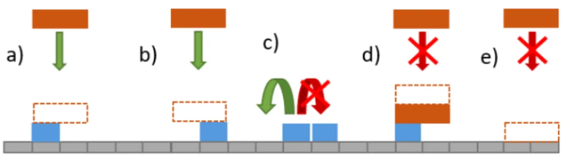
In Fig. 2.2 some of the rules of the model are represented for a simple case where Spatch = 1

(monomers) and Spart= 2. From left to right are, the patch diffusion and particle adsorption, as well

as two prohibited processes which are the particle overlap and particle adsorption on empty space of the substrate.

Figure 2.2: Representation of the rules of the model. In blue are the DNA patches which are modeled as monomers that are diffusing on the lattice, in green are the colloidal particles which are represented as squares with length Spart= 2 in units of lattice sites, and adsorb on top of free patches. The first two processes a) and b) are allowed and correspond to the patch diffusion and particle adsorption, c) and d) are prohibited which correspond to the overlap of particles and the adsorption on empty space of the lattice.

In this thesis, we will study this model in two and one dimensions, the only difference for one dimension is that the patches are restricted to move along a line (instead of a plane). Our study focuses on the simple case where Spatch = 1 and Spart = 2, this can be a good approximation to

the experiments in the case where the size of the colloidal particles are much larger than the ones of the DNA patches so that every patch is fully covered by a particle. It is also important to note that

(23)

for this choice of parameters it is impossible to form clusters, since there can never be more than one particle per patch. We will focus mostly on the study of the time dependent dynamics as well as the jamming state, which corresponds to the state where no more particles can adsorb (no more free patches available).

This model is related to the classical Random Sequential Adsorption (RSA) model [40–52]. Here, we have the random irreversible adsorption of particles of a given size, which interact by excluded volume, similar to other RSA models. The main difference is the fact that they only adsorb on free mobile patches.

(24)

(25)

Chapter 3

Numerical implementation

Ideally, simulations should reproduce natural phenomena in the most accurate way. Unfortu-nately, just by estimating the computational power necessary for simulating even the simplest sys-tems, we realize that this is impossible. For example, consider a mole of an ideal gas in a cubic box. To track the trajectories of every single particle in this system, it would be necessary to save all their positions in the memory of the computer. A mole corresponds to 1023atoms, so we would need at least 1024 bytes. Besides, it would also be necessary to know all their velocities, so another 1024 bytes would be required. This amount of memory space is currently unavailable, thus, new methods are needed to access the relevant time and length scales, while still grasping the relevant physics.

After elaborating a model that is able to capture the important properties of a physical system, it is necessary to study it. One way is analytically, where one uses mathematical tools to describe the system, but for the systems that we are studying here, which are far from equilibrium, an exact analytical approach is rarely possible. So most findings are numerical, and thus numerical tools and algorithms are necessary.

To construct an efficient algorithm there needs to be a great understanding of the problem at hand. An efficient algorithm needs to lead us to results that are as accurate as possible in a reasonable amount of time. The best approach is to reduce the number of irrelevant instructions, which in turn reduces the required computational effort. For that, the most important step is to define the time and length scales where relevant processes occur, because only then it is possible to device a model and algorithm that grasps the most relevant features of the problem in an efficient manner.

This first step was already presented in chapter 2, where we gave a thorough description of the model and all the processes of relevance. With this information, we find a technique that best adapts to our problem. It is important to note that we are dealing with a model, where fluctuations play a relevant role, and so randomness needs to be taken into consideration. Thus, a statistical description of the possible outcomes is the meaningful approach to the problem in opposition to a deterministic one. The most common techniques are Brownian Dynamics and Monte Carlo methods.

Brownian Dynamics (BD) consists of calculating the individual trajectories of all the particles in the over damped regime. For this, it is necessary to know the initial conditions, and also how they interact with each other so it is possible to calculate the forces between them. Currently, these requirements are not restrictions, since even by limiting the amount of particles one can simulate at a given time, it is possible to generate enough data to improve the statistics (in a reasonable time frame). Other than that, there are also many techniques that make use of efficient algorithms [53, 54] to increase the quality of the statistics, for example, a popular approximation to use is to, instead of considering the interaction between all pairs of particles, only consider pairs of particles within

(26)

Chapter 3. Numerical implementation

a cut-off radius. This kind of approximation considerably increases the efficiency of the algorithm without notably affecting the results. But for each case, it is necessary to evaluate which degrees of freedom are relevant and which ones can be coarse grained. First, the interactions between all the constituents of the model can be simply described as excluded volume, so the advantage that this technique has of always taking into account the particle-particle interactions is not relevant for us. Second, as stated in the previous chapter, the adsorption of the particles occurs in a much larger timescale than the particle dynamics on the surface of the droplet, therefore we consider that it is not necessary to consider the motion of particles. Finally, the worst disadvantage of this technique is the time scales that are reachable. A standard BD simulation has typical time steps of the order of 10−7s, so if we want to study events that happen in time scales of the microsecond (or larger), the computational power necessary becomes too demanding for current computers.

We decided to consider a Monte Carlo (MC) method, instead. This makes use of random sam-pling to compute the average of the different observables [55]. This is a more suited technique for our approach since it reduces the complexity necessary to implement BD (with MC it is not necessary to explicitly calculate the trajectories of the particles towards the substrate but solely considers an effec-tive adsorption rate), and also, since we want to study the long time behavior, by using MC we can reach the final configuration of the system in a more reasonable time frame. But we did not use the standard MC method, we chose a more specific method named kinetic Monte Carlo (kMC). Standard MC does not take into account the physical time of the simulation nor the sequence of events leading to the final configurations. This is a problem when studying an out-of-equilibrium system, because the relevant physical properties depend on the kinetics leading to the final configuration. Thus, we use kMC, since it has a physical clock and the sequence of events corresponds to a possible sequence of events in the physical system [56–58]. The obtained configurations are not necessarily the ones with the lower free energy (the ones obtained in equilibrium through MC), but the ones obtained kinetically.

With kMC it is possible to formulate a rejection free algorithm that improves the overall per-formance of the simulations, when compared to standard MC. For this, we only need to know the rates for all the processes and, as described in the previous chapter, this is set by the model. Another relevant advantage of it is that it lets us define a physical time, which is a very important property when studying the kinetics of adsorption and when comparing to experimental results. To define the physical time it is necessary to relate the rates used in the algorithm with the ones measured experimentally.

3.1 Kinetic Monte Carlo

The algorithm, for the kMC, was coined N-fold way since processes are classified into N different classes, based on their transition probabilities, or rates in our particular case. It was first proposed by Bortz, Kalos and Lebowitz, in 1975, for the simulation of Ising spins [59]. At that time, the problem they faced was that, for low temperatures, the amount of rejections the MC algorithms needed to simulate the system was very large, which means that there would be many irrelevant steps before the relevant physical properties could manifest. Thus, they introduced a rejection free algorithm to address this numerical challenge.

Since we are dealing with a stochastic model, the dynamics of the components will be random between different simulations, even for the same set of parameters. Thus, if we analyze the data from a single evolution, the results can display distinct features that are not characteristic of a typical

(27)

evolution and are only a product of statistical fluctuations. To avoid these features, when measuring the results, the quantities of interest are taken by averaging over many samples.

The algorithm starts by generating a two-dimensional square lattice with size L in units of lattice sites (as explained in chapter 2). Then this lattice needs to be occupied by a certain density of patches. Thus, it is necessary to generate a random configuration of free patches distributed in an uncorrelated fashion. We use the random number generator (RNG) Marsenne Twister from the Boost C++ Libraries, to generate pseudo-random numbers. We chose this RNG because it has a very long period (219937− 1), which means that it is necessary to make a high number of iterations for the RNG to start repeating itself, and also, it has passed numerous tests for statistical randomness [60].

The first step of the algorithm is to define which processes can happen, in our case (using the model in Chapter 2) we have patch diffusion and particle adsorption, but since the lattice the patches need to be distributed, another process is introduced, which is the patch adsorption. To make this simpler, the simulation is divided into two parts, a first one where the patches are adsorbing on the lattice and at the same time diffusing (after adsorption) and a second one where we have the necessary density of patches already adsorbed, which we define as n0, and so the particles are allowed to adsorb

while the patches stop, and are only allowed to diffuse. The diffusion coefficient rate is always set to a given value, since the patches are allowed to diffuse in both the first and second part of the simulation. The reason why we let the patches diffuse while they are adsorbing is so that their initial distribution is uniform and does not depend on the adsorption sequence.

3.1.1 Initial conditions

As stated, the simulation is divided into two parts, the first corresponds to the adsorption of the patches on the substrate, and represents the initial conditions. To implement this, we use the kMC algorithm.

First, a catalog of all the possible processes that can occur is created. For that it is necessary to sweep all lattice sites to identify what processes can happen in them. Since the lattice starts without patches, the only process that can happen is patch adsorption, therefore the catalog corresponding to that process will have all lattice sites in it, while the catalogs for the other processes are empty. Thus, a patch is adsorbed, and for that a random number is generated between 0 and the size of the catalog that corresponds to the process of patch adsorption, and the patch is generated in the site corresponding to that, randomly selected, entry in the catalog.

After a process is performed the catalogs need to be updated since the system configuration has changed. After a patch adsorbs, a new one cannot adsorb in that site, so the entry corresponding to it in the patch adsorption catalog is removed. As stated previously, in this first part of the simulations, we want the patches to diffuse, therefore we add an entry to the patch diffusion catalog corresponding to this site. To increase the efficiency of the algorithm, we start to build the catalog of particle adsorption as well, during this first part, so an entry is also added to it, since this patch is free. It is important to note that, although the particle adsorption catalog starts being developed in this part, it will only be taken into account in the second part of the simulation, since the particle adsorption rate, in this first part, is set to zero. It is also necessary to update other sites that are affected by this patch, for example, if Spatch= 1 and Spart= 2, then after the patch adsorbs the first and second neighbors

of this site also need to be added to the particle adsorption catalog since one can adsorb there and still touch the patch.

(28)

which process to perform next, the cumulative rate is calculated:

Ci= i

X

j=1

njWj , (3.1)

where njis the number of components that can perform a certain process j, and Wj the rate for that

process. CN, where N is the total number of processes, is the total rate. Since currently we only

have two processes, N = 2,

CN = N

X

j=1

njWj = nP AWP A+ nP DWP D , (3.2)

where PA corresponds to the process of patch adsorption and PD to the one of patch diffusion. To select the next process, a random number, r, uniformly distributed in the interval ]0, 1], is generated and the process is chosen by finding the i which satisfies the inequality:

Ci−1< rCN < Ci , (3.3)

then the process is performed by selecting the respective catalog and generating a random number between zero and the total number of entries in it, the entry selected will correspond to a specific site on the lattice that will perform the process. Finally, the different catalogs are updated. This way, no rejection occurs, which leads to an increased efficiency of the algorithm.

This algorithm is iterated until the density of patches reaches n0. After this happens, the initial

conditions are generated. The time and the rate of patch adsorption are set to zero, and the rate of particle adsorption is increased.

3.1.2 Algorithm for the kinetics of adsorption

When the initial conditions of the model are generated, which corresponds to a density of n0

patches adsorbed, the second part of the simulation begins. This corresponds to the particle adsorp-tion on the free patches which are diffusing on the substrate. As menadsorp-tioned, to increase the efficiency of the algorithm, we construct the catalog for patch adsorption while generating the initial condi-tions, but we did not take it into account when evaluating the possible processes in that part. Now it is necessary to do so.

Since both catalogs (patch diffusion and particle adsorption) are already constructed, it is possible to perform a process. For that, the cumulative rate is calculated again, as presented in Eq. 3.1, but now the processes possible will be different when calculating the total rate:

CN = N

X

j=1

njWj = nP tAWP tA+ nP DWP D , (3.4)

where PtA corresponds to particle adsorption and PD is patch diffusion. A new random number is generated and the process is chosen by using Eq. 3.3, but now with the values from Eq. 3.4. Then the process is performed by selecting the respective catalog and generating a random number between zero and the total number of entries in it, the entry selected will correspond to a specific site on the lattice that will perform the process. After the catalogs are updated, the algorithm is iterated.

(29)

3.1.3 Time incrementation

Since we are interested in studying the time dependent dynamics, time needs to be incremented in the appropriate way.

Given a certain time increment ∆t, P (∆t) is defined as the probability of no process occurring in the interval ∆t after a previous one has occurred, and CN as the total rate of events, as defined

previously using Eq. 3.1. Thus, the probability of a process to occur in the interval dt is CNdt. The

probability of a process to occur in the interval [∆t, ∆t + dt] is proportional to the probability of no process during ∆t and the probability of a process occurring in the interval dt. Therefore, the probability of no process in ∆t + dt is given by [61]:

P (∆t + dt) = P (∆t) − P (∆t)CNdt . (3.5)

Solving Eq. 3.5,

P (∆t) = exp(−CN∆t) . (3.6)

From Eq. 3.6, one gets:

∆t = −C_N−1ln(r0) . (3.7)

where r0is a random number, uniformly distributed, in the interval ]0, 1].

3.1.4 Boundary conditions

Since we are interested in properties that happen in the bulk, it is necessary to guarantee that boundary effects are negligible, to reduce finite-size effects. Experimentally, the number of particles is large enough, so that many times, it is a good approximation to treat the system as if it was in the thermodynamic limit. However, as discussed previously, due to computational constraints, it is not possible to numerically replicate such scale of events, and we have to limit the size of our simulated system. A good approach is to use periodic boundary conditions. This means that each side of the substrate, in our case, is mapped into the opposite one. Thus, if a particle diffuses through one of the sides it will re-enter the system in the opposite side. By doing this, we are effectively considering an infinite system, where the substrate is replicated periodically. If one wants to measure the distance between sites it is necessary to take the boundary conditions into account and make the proper mapping.

It is important to stress that, although the use of periodic boundary conditions helps in reducing the finite-size effects, it might not make them negligible. Thus, it is still necessary to take these effects into consideration when measuring the relevant properties. For that, we need to make sure we are not using a system size that is too small, to the point the effects are noticeable. Thus, it is important to study the properties of interest for different system sizes. By observing when the measurements collapse to the same values, we can conclude what size we can consider so that the finite-size effects are negligible.

The algorithm explained here focused more on the use of a two-dimensional substrate, but it is also possible to adapt it to the one-dimensional case. The differences come mostly from the reduction of the possible directions, from four to two.

(30)

3.2 Code validation

After formulating an algorithm and writing the code, it is necessary to test it to check for possible problems in the implementation. In this section, results taken with the algorithm described previously are compared to known analytical and numerical results. First, we study a one-dimensional case with only the adsorption of dimers on a lattice. Then, we compare a two-dimensional implementation to the adsorption of monomers with diffusion on a lattice, using the algorithm described in the previous section, to analytical results.

3.2.1 Dimer adsorption on a one-dimension lattice

A very well known exact result in RSA is the random sequential adsorption of dimers [62, 63]. The interesting property of this system is that a vacant region that is smaller than the particle size (in this case dimers) can never be filled, which means that the substrate can reach a jammed state that cannot accommodate additional adsorption events, where the substrate is not completely covered. So it is interesting to study how the system approaches the jamming state.

The model is simple, there is a flux of particles (dimers) to the substrate, attempting to adsorb irreversibly. These adsorption attempts occur at random on the substrate, and dimers cannot overlap with each other. After each successful adsorption attempt, the coverage of the system increases, where coverage is defined as the density of occupied sites. From here, it is possible to conclude that the jamming state coverage is between 2/3 and 1. The first corresponds to the case where there is always an empty site on the left and right of an adsorbed dimer, and the second, to the case where there are no empty sites in the lattice and, therefore, all are filled. A first result was derived by Flory [64] using a combinatorial approach, where he derived that an initially empty substrate saturates at a jamming coverage: ρjam = 1 − exp(−2). It is also possible, using an empty interval

method to reach an exact analytical solution for the time dependence of the coverage, ρ [62, 63]:

ρ(t) = 1 − exp{−2[1 − exp(−t)]} . (3.8)

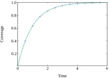
In Fig. 3.1 is plotted the coverage as a function of time. In circles are the simulation results using the algorithm described in the previous section, where the only possible process is the adsorption of dimers on the substrate, and in dashed lines are the theoretical results, in green is the value for the coverage of the jammed state derived by Flory, while in blue is the exact solution in Eq. 3.8.

The results were taken for a substrate of size L = 107, in units of lattice sites. From Fig. 3.1, it is possible to conclude that our simulation results are in perfect agreement with the analytical ones. Using our simulation results, we reached a value of the jamming coverage equal to 0.864666 ± 8 × 10−6, which is in very good agreement with the analytical one, ρjam = 1 − exp(−2) ≈ 0.864665.

3.2.2 Adsorption of monomers with diffusion on a two-dimension lattice

As the dimension increases the problem becomes increasingly difficult. While there are exact analytical results for RSA in one-dimension, there are practically no exact solutions for two and three dimensions. This is mostly due to the complexity of the problem, since it is necessary to take into account all possible configurations of connected clusters of any size and then solve the coupled equations for the evolution of the probabilities that each cluster configuration is empty. Thus, most results are either achieved using simulations, or approximations like mean-field.

(31)

Figure 3.1: Coverage as a function of time, for dimer adsorption in a one-dimensional lattice. In circles are the simulation results, and in dashed lines are the theoretical results, in green is the value for the coverage of the jammed state derived by Flory, while in blue is the exact solution in Eq. 3.8.

To test our two-dimensional implementation using an exact analytical solution, it is necessary to consider simple systems. In this case, we simulate the adsorption of monomers on a two-dimensional lattice. The model is pretty straightforward, monomers attempt to adsorb on a two-dimensional lattice with a certain flux, and after adsorbing, they are allowed to diffuse to their nearest neighbors if they are empty. The adsorption is considered irreversible and the monomers cannot overlap.

This next step of the code validation is meant to test our implementation with more than one possible process. Although the particles can adsorb and then diffuse, since we are dealing with monomers, the diffusion coefficient should not be a relevant parameter. So the coverage needs to evolve as it would be expected for monomer adsorption only, which means that the density of occu-pied sites increases with time at a rate proportional to the density of vacancies:

dρ

dt = 1 − ρ , (3.9)

solving this equation we get:

ρ(t) = 1 − exp(−t) . (3.10)

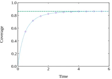
In Fig. 3.2, it is plotted a comparison between this solution (Eq. 3.10) and the simulation results, for a two-dimensional substrate with length L = 1000, in units of lattice sites. It is possible to observe that the diffusion coefficient does not play a role in the results and therefore our simulation results are in perfect agreement with the analytical ones.

(32)

Figure 3.2: Coverage as a function of time, for monomer adsorption in a two-dimensional lattice. In circles are the simulation results, and in a dashed line is the theoretical result derived for monomer adsorption given by Eq. 3.10.

(33)

Chapter 4

Adsorption kinetics on a lattice

Our main objective is to study the kinetics of adsorption of colloidal particles on mobile patches, that diffuse on the surface of an oil droplet. For this, a model has been presented that tries to capture the most relevant physical features (see Chapter 2). We also already presented the method and algorithm we will be using to simulate it (see chapter 3). In this chapter, the results are discussed.

First, we discuss a one-dimensional case of the model presented in Chapter 2, where the particles are represented as dimers, Spart = 2, and patches as monomers, Spatch= 1. One thing to note in this

case is that since the patches are monomers only one particle can adsorb on them. This means that for this set of parameters no clusters are formed. This corresponds to the limit where the colloidal particles are much larger than the patches, to the point where there can only be one particle per patch adsorbed. We will focus on the time dependent dynamics of the coverage and the jamming state. We will study also how they vary with the relevant parameters of the model, which are the patch diffusion coefficient and the flux of particles towards the substrate.

In this chapter, we will also consider the two-dimensional case. What this means is that the patches have one more degree of freedom, and the particles instead of being modeled as dimers, are squares.

We also discuss a mean-field approach to the model, to describe the time evolution of the den-sity of free patches and adsorbed particles using rate equations. With it, we can reach closed form equations for this time dependence, which are in very good agreement with the numerical results.

4.1 Kinetics on a one-dimensional lattice

In this section, we consider the adsorption of dimers (Spart = 2) on monomers (Spatch = 1).

In Fig. 4.1 there is a scheme summarizing some rules of the model in one-dimension. The model described in Chapter 2 is the same as the one used here, the major difference comes from the fact that the translational degrees of freedom are reduced.

In this case, there are only two possible configurations of complexes: one particle and one patch; or one particle and two patches. Therefore, it is not possible to form clusters, since on each patch there can only be one particle adsorbed. If we define the coverage, θ, as the density of complexes formed (number of adsorbed particles per lattice site), then, the maximum coverage is equal to the initial density of free patches. If the flux F is large enough, the diffusion of the patches is negligible, and the system is sufficiently diluted, then:

(34)

Chapter 4. Adsorption kinetics on a lattice

Figure 4.1: Representation of the rules of the model for one-dimension. In blue are the patches which are represented as segments of length Spatch= 1, in units of lattice sites and can diffuse on the lattice, with a certain diffusion coefficient. In orange are the particles which are represented as segments of length Spart= 2 in units of lattice sites, and adsorb on top of free patches. a) and b) represent the allowed adsorption processes for this particular pair of Spatchand Spart, then c) is a representation of the rules of diffusion for patches, d) and e) are the prohibited processes for particle adsorption.

lim

F →∞θj → n0 , (4.1)

where θj is the jamming coverage, defined as the asymptotic coverage when there can be no more

adsorption events (all free patches are occupied), and n0is the initial density of patches. We are also

able to deduce another limit, where each particle has two patches. In this case, θj → n0/2, which

corresponds to a case where the time the patches have between adsorptions is so large that they are always able to aggregate to a particle-patch complex (D >> F ).

Unless otherwise stated, all results are obtain for a substrate size L = 107, and averages over 104 samples.

4.1.1 Time dependent dynamics

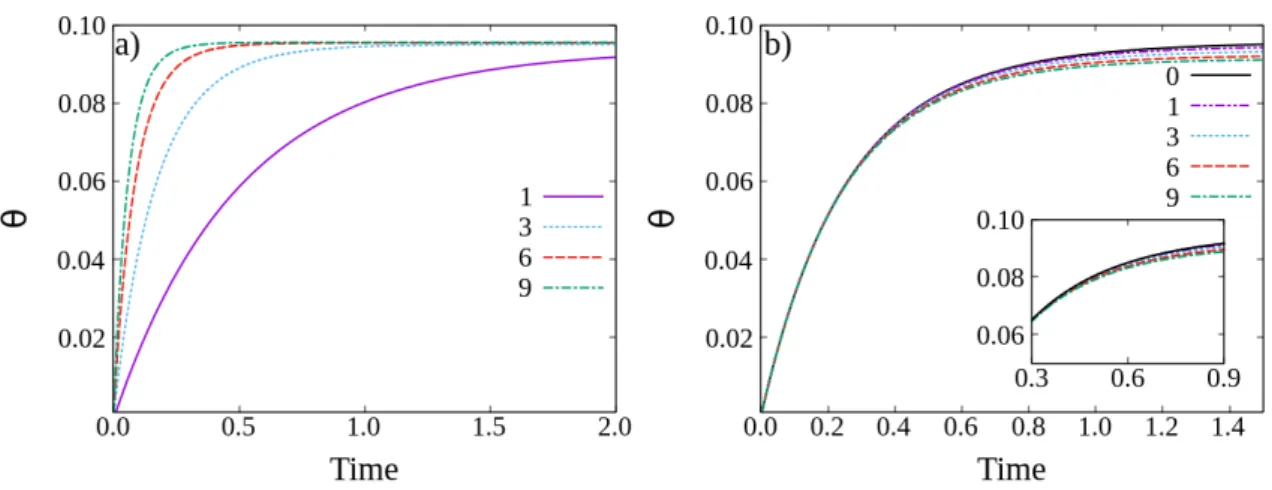
The results are presented in Fig. 4.2, where a plot of the coverage as a function of time for a given F and D is shown. From Fig. 4.2 a), it is possible to see that the jamming coverage increases with F . As F increases the patches will have less time to diffuse during successive adsorptions, and therefore it will be more likely that a particle adsorbs on a free patch than the patch aggregating to an already adsorbed particle. As expected, when F increases the coverage will tend to the maximum value given by 4.1. In Fig. 4.2 b) it is observed that the jamming coverage monotonically decreases with D. In this case, the patches will have more time between adsorptions and therefore their probability of aggregating to a complex is higher which in turn will decrease the jamming coverage.

From Fig, 4.2 b), we can see that the curves in the initial dynamics show the same behavior and then after a certain time they diverge from each other. If we lower the initial density of patches this effect is even less noticeable, as seen in Fig. 4.3 a), for n0 = 0.03. It is also possible to observe that

as the diffusion coefficient increases the faster the curves deviate from each other (Fig. 4.3 b). We argue that the patches, for low times, do not have enough time between adsorptions to ag-gregate to complexes and therefore the effect the diffusion of the patches has on the coverage is negligible. This is confirmed when we compare the simulation curves for D > 0 with one for D = 0. It is possible to observe two different regimes, the first where the diffusion coefficient of the patches does not seem to impact on the coverage (all curves almost overlap with the one with D = 0), and the second where there are significant differences. The first regime corresponds to a

(35)

Figure 4.2: Time-dependence of the coverage for a) D = 1 and F = 1, 3, 6, 9, b) F = 2 and D = 0, 1, 3, 6, 9. The initial patch density is n0= 0.1. It is possible to observe on a) that, as F increases the jamming coverage tends to the maximum value given in Eq. 4.1 and on b) that when D is increased the jamming coverage decreases. From b) we can also see that for the initial dynamics the curves almost overlap when F is constant which means that in this regime the system behaves as D ≈ 0.

Figure 4.3: Time-dependence of the coverage for F = 2 and D = 0, 1, 3, 6, with n0 = 0.03, in a), and F = 2 and D = 0, 3, 30, 90, with n0 = 0.1, in b). By comparison to Fig. 4.2, we can see that as n0decreases the curves will stay longer in the first regime where the system behaves as D ≈ 0. As D increases it is possible to observe that the curves diverge sooner from the D = 0 one.

system where D ≈ 0, while in the second the diffusion of the patches starts to have a larger impact on the coverage evolution. This also explains why for smaller n0the curves deviate less from D = 0,

because as n0decreases the typical distance between patches, and between complexes and patches,

will increase, which means that they need more time to find complexes, and so the first regime lasts for a longer period of time.

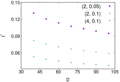
We define a t∗ as an instant of time where the coverage for a certain diffusion coefficient D differs from the one for D = 0 by more than ε.

|θD(t∗) − θ0(t∗)| = ε . (4.2)

Here, we considered ε = 0.01. θD is the coverage for a given diffusion coefficient D and θ0 is

the coverage for D = 0. From Fig. 4.4 one can observe that as D or n0 increases, t∗ decreases,

(36)

4.4 is that t∗decreases when F increases, since the higher the value of F the more particles will be able to adsorb and therefore it will be more likely for a patch to aggregate to a complex, since there are more available. Below, in section 4.3 we will provide a theoretical study to explain this behavior.

Figure 4.4: t∗as a function of D, for different sets of parameters (F, n0) = (2, 0.05); (2, 0.1); (4, 0.1). It is possible to observe that when (F , D and n0) increase, t∗decreases.

4.1.2 Jamming state

Fig. 4.5 shows the coverage evolution for different values of F and D. It is clear that, while the kinetics depend on both values, the jamming coverage only depends on the ratio F/D, as for the same ratio the curves overlap asymptotically.

Figure 4.5: Coverage as a function of time for different F and D. It is possible to observe in the insets that when F and D change but the ratio F/D is kept the same, the curves collapse when they reach jamming.

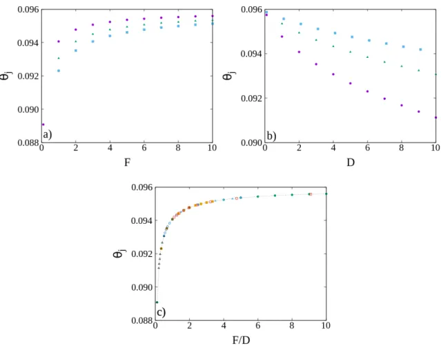
From Fig. 4.6 a), it is possible to observe that θj (jamming coverage) increases monotonically

(37)

Figure 4.6: Jamming coverage as a function of a) F for D = 1, 2, 3, b) D for F = 2, 5, 10, both represented as circles, triangles and squares respectively, and c) the ratio F/D. As expected from the previous results, the jamming coverage decreases with D but increases with F . Other than that by using the parameter F/D instead, it is possible to observe a data collapse.

particle per patch, as expected.

Using the results from Figs. 4.6 a) and b), but now plotting θjas a function of the ratio F/D, we

get a data collapse (Fig. 4.6 c). Thus, we are able to confirm, for a wider range of parameters, the result in Figure 4.5, that θj will only depend on the ratio F/D, and not on the pair F and D.

It is possible to observe that the jamming coverage increases monotonically with F/D. This happens because when F/D is small, the patches will have enough time to find complexes and aggregate to them between successive adsorptions, reducing the number of free patches available while not increasing the coverage. On the other hand, when F/D is larger, the patches have less time to diffuse and so more particles will be able to adsorb, which will lead to a more efficient (jamming) coverage. This effect is even more pronounced for higher initial patch densities where the typical distance between patches, or between patches and adsorbed particles, is shorter, favoring the binding of free patches to previously adsorbed particles.

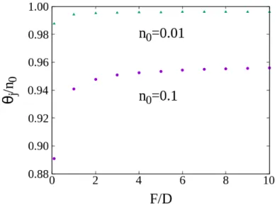
In Fig. 4.7 the jamming coverage as a function of F/D is shown, for n0 = 0.1, 0.01. It is

possible to observe that as n0decreases, the jamming coverage increases. This is due to the fact that,

when n0increases the typical distance between patches, and between patches and adsorbed particles,

(38)

Figure 4.7: Jamming Coverage as a function of F/D for n0= 0.1, 0.01. It is possible to observe that as n0decreases the jamming coverage increases.

4.1.3 Finite-size study

To be able to simulate these systems in a reasonable time frame it is necessary to take into account some approximations and limit their size. Then, one of the problems that can arise is the effect of the finite size of the system in the results. These are unwanted effects, since in the real systems they are typically not relevant (they are usually near the thermodynamic limit). Thus, it is necessary to see if the results presented here can be a byproduct of the finite size of the system.

To verify if there are any finite-size effects in our results we consider three different system sizes, L = {105, 106, 107}. The results are presented in Fig . 4.8. It is possible to conclude from this analysis, that there are no relevant finite-size effects in the results. Thus, we can focus our study on only one system size (the largest one).

Figure 4.8: Jamming coverage as a function of the ratio F/D (a), and coverage as a function of time (b), for different systems sizes, L = {105, 106, 107}. It is possible to observe that all curves collapse and therefore there are no relevant finite-size effects that we need to take into account.