J. Braz. Soc. Mech. Sci. & Eng. vol.28 número1

Fábio S. de Oliveira

Jurandir I. Yanagihara

Antônio L. Pacífico

Film Thickness and Wave Velocity

Measurement Using Reflected Laser

Intensity

The objective of this work is to develop a film thickness and velocity measurement technique using laser intensity measurement in liquid film flow. This technique was developed for annular flow studies, but it has been scarcely used due to the equipment's complexity, as compared with other techniques. The laser technique uses the reflection of the laser beam in water interface and the attenuation of its intensity to determine the interface position. Thus, the relation between intensity and thickness must be obtained by calibration. A theoretical model was proposed for the optical phenomena present in the film thickness measurement and its results were compared with experimental results using a planar mirror. A controlled experiment was conducted using one-dimensional waves in a short channel where the wave frequencies were varied by changing the vibrator's frequency and the film thickness was modified by changing the liquid volume. The reference film thickness was obtained by the analysis of photographic data taken through the transparent channel walls, allowing the comparison to the results from the laser technique. The experimental results for the film thickness presented a good agreement with the reference thickness from photographic data. The interface wave propagation velocities were measured with good accuracy, showing good agreement with the theoretical data. Keywords: Film thickness, laser intensity, wave velocity, optical method

Introduction

The instrumentation used to measure film thickness in annular flow usually utilizes conductivity principles that are normally affected by the temperature and concentration of electrolytes, as shown in the work of Fukano (1998). In some cases, like those techniques that utilize wires emerged in the flow as conductive probes (Koskie et al., 1989), the probes may cause interference in the measured flow. According to Kang and Kim (1992), the presence of wires in the flowpath produces results that are not so reliable, mainly because meniscus formation may affect the readings. 1

As the electrical permittivity varies less with temperature than the electrical conductivity, as mentioned by Geraets and Borst (1988), capacitive methods solve problems related to invasive techniques, but capacitive techniques always provide local average values.

Otherwise, ultra sonic techniques, as described in Kamei and Serizawa (1998), are local techniques and are independent from variation of the electrical properties of the working fluid during the experiments. However, the uncertainty associated with this technique is directly related to the ultra sonic wavelength (in this case 75 µm). The uncertainty of this technique is high when compared to other techniques.

Fukano (1998) described a local probe that utilizes constant current technique that provides lower values of the uncertainty but, as already discussed, it presents the problem of variation in conductivity when temperature varies. This probe also presents limitations for the measured film thickness. If the film thickness is thinner than the distance between the two probes, the measured result does not present acceptable uncertainty. There is also another limitation that is the maximum film thickness that can be measured with a given probe, due to its dimension.

The fluorescence-based techniques, as described in Hewitt et al. (1978), are essentially local techniques and in some cases the fluorescence effect can be stimulated by laser, as described in

Paper accepted October, 2005. Technical Editor: Aristeu da Silveira Neto.

Driscoll et al. (1992). The concentration of fluorescent material must be controlled to avoid its saturation.

Laser beams can be used to measure film thickness using attenuation of intensity due to the absorption by the fluid. Samenfink et al. (1996) describes a system that measures film thickness and interface inclination, but despite the possibilities of such technique, it requires that the flow occurs in an open channel to install optical detection equipment in the opposite side of the laser beam source. Thus, this technique cannot be applied to annular flow. The utilization of laser attenuation is described in Ohba et al. (1992) where the radiation reflected by a gas-liquid interface is measured. The variation in reflected radiation intensity is related to film thickness. The major advantage of this technique is that the flow is not disturbed. The measurement of reflected total flux is made through the same optical fiber that launches the laser to the measurement point. The intensity of the reflected ray that returns by the optical fiber is directed to a photodetector that measures its intensity. This technique only detects the thickness when the interface is parallel to the tip of the optical fiber. When the interface is parallel, the equipment detects a signal peak. This peak is observed only when a peak or a valley of a wave passes over the optical fiber tip.

Yu and Tso (1995) proposed to use various optical fibers, one central to launch the laser on the measurement point and others, equally spaced around it, to detect the radiation reflected by the gas-liquid interface. The objective is to overcome the limitation involved in the one fiber probe. As described, the one fiber probe only detects film thickness when the interface is parallel to the optical fiber tip. Yu and Tso (1995) concluded that with the new multi fiber probe it is not possible to measure inclination of gas-liquid interface, but the probe increases the range of thicknesses that could be measured by the reflected laser intensity technique to 4 mm thickness (four times the previous range that was up to 1.5 mm).

J. of the Braz. Soc. of Mech. Sci. & Eng. Copyright  2006 by ABCM 31 The objective of this work is to develop a film thickness and

velocity measurement technique using the laser intensity attenuation principle. A theoretical model is proposed and the numerical results of the model are compared with the results of a simple experiment using a planar mirror. A controlled experiment is conducted using one-dimensional waves in a short channel where the wave frequencies are varied by changing the vibrator’s frequency and the film thickness is modified by changing the liquid volume. Analysis of photographic data taken through the transparent channel walls allows the comparison with the results taken by the laser technique. The interface wave propagation velocities are also measured.

Nomenclature

b = optical fiber core diameter, mm

d = distance, mm

e = Napier base, dimentionless

g = acceleration of gravitiy, m/s²

h = film thickness, mm

I = laser intensity, W/m²

i = current, A

l = film thickness in optical fiber axis direction, mm

N = number of samples, dimentionless

R = laser beam radius, mm

r = radial position, mm

v = wave velocity, m/s

x = axis of retangular coordinates, mm

y = axis of retangular coordinates, mm

z = axial position, mm Greek Symbols

θ = aperture angle of the laser beam, rad φ = interface inclination angle, rad

ψ = angle formed by radiation vector and optical fiber axis Subscripts

0 = related to origin in the surface of optical fiber

CL = related to center line, over the axis of optical fiber

f = related to liquid film or in the optical fiber position

mirror = related to mirror position

p = related to wave peak

r = related to radial position

z = related to the direction from origin of laser beam to (r, z) = point

* = related to measurement on the optical fiber tip

Description of Technique

The proposed experimental apparatus is sketched in Fig. 1. Optical fibers with 500 µm core diameter are used in the experiment. They present good installation properties and increase the measurement range as compared with the fibers with core diameter of 50 µm and 80 µm tested by Ohba et al. (1992) without having to increase the number of optical fibers.

In order to launch the laser radiation in the optical fiber and to detect the reflected radiation, an optical arrangement is used to adjust laser radiation properties. As can be seen in Fig. 1, only one laser source is used. By using a beam splitter, the original beam is divided in two. The two emerging beams have their intensity adjusted by a half wave plate placed between the laser and the first beam splitter. Both beams are launched on microscopic lenses that focalize them in the tips of the 500 µm core diameter optical fibers. The optical fibers conduct the radiation to the measurement point. The radiation emerges from the opposite tip of the optical fibers, travels across the water film and reaches the interface. The major part of the radiation is transmitted through the interface, but a small

portion reflects back to the optical fibers. The reflected radiation emerges at the other end of the optical fiber, passes through the microscopic objective lenses, and is reflected by the beam splitters to a second microscopic lens that focalizes each beam in its respective photoconductive diode PIN.

The current drained by a PIN photodiode is transformed in voltage signals by two amplifiers that send their signal to an oscilloscope. The oscilloscope has a RS-232 port that can be read by a computer.

The optical fibers are installed in the measurement point with 3 mm distance between them in the interface wave propagation direction. Thus, the film thickness is measured by both optical fibers and the resultant signals can be used to calculate the correlation coefficient to determine the wave propagation velocity.

A wave generator was built to generate one-dimensional waves in order to create an appropriate measurement condition. Due to the channel dimensions and the surface meniscus, the reflection of the waves was considered negligible and no caution was taken with respect to this disturbance. The wave generator was built using a step motor that was activated by a transistors’ bank connected to a logical sequencer. The frequency was controlled by a clock generator microchip. The clock frequency depends on an external resistor that in this case was a potentiometer. The shaft of the step motor was connected to a crank, which transmitted the oscillatory motion to the wave generator plate.

Figure 1. Lay out of optical arrangement used to launch radiation in optical fiber.

The wave generator was installed over an adjustable level platform in order to allow the positioning with respect to the channel bottom.

Figure 2. Arrangement of the wave generator and the schematic view of the channel.

Figure 3. A view of optical fiber installation.

Figure 4. Waves traveling through the channel.

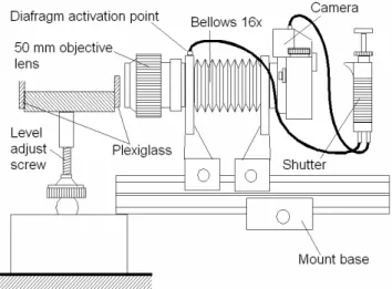
In order to have a reference thickness value, pictures of the film at the measurement point were taken to compare with the measured results. The scheme of Fig. 5 shows the camera installation at the side of the test channel. The walls of the test channel were built of plexiglass to allow visualization of flow through the walls. A device, shown in Fig. 5, was used to amplify the local image of the optical fiber tip.

Figure 5. Installation of photographic camera in the side of test channel.

Theoretical Model

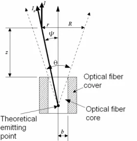
The total flux detected by the optical system can be calculated by intensity integration using mirror symmetry principles. The intensity can be integrated over the area of the optical fiber tip image. By knowing the position of the interface (distance and inclination), it is possible to determine the position of the image using symmetry principles. The integration of the laser flux radiation that passes through the area was based on the position of the tip image in space. Fig. 6 shows the position of the image.

Figure 6. Position of optical fiber image obtained by symmetry principles.

The intensity flux distribution of a laser beam, according to Ohba et al. (1992), follows a Gaussian distribution curve. The equation that describes this curve is given below:

( )

( )

2 4

, Rz

r

CL z e

I z r I

⋅ −

⋅

= (1)

J. of the Braz. Soc. of Mech. Sci. & Eng. Copyright  2006 by ABCM 33 intensity in the center of laser beam and I(r, z) is the local intensity

inside the laser beam. The laser beam that emerges from the optical fiber has the same distribution curve.

The flux in the center of the laser beam ICL(z) is given by:

( )

_{( )}

₍

₎

0

1 4

−

− ⋅ ⋅ π

⋅ =

e z R

I z

ICL (2)

where I0 is the total flux that passes through the radiation emitting

device or the tip of the optical fiber. Figure 7 shows a schematic view of the geometric model and Fig. 6 shows the symmetry principle used. It can be seen the angles and the radiation components involved in the calculation of the radiation over the optical fiber image.

Figure 7. Schematic drawing that shows the radiation components as well as the angles involved in the integration of the intensity flux.

The intensity flux Ir(r,z) can be obtained through some algebraic

steps as:

( )

_{( )}

₍

₎

_{( )}

2 2 4

0

2 tan 1

1 4

, _

  

 

     θ ⋅ + ⋅ − ⋅ ⋅ π

⋅ ⋅

= ₋

⋅ −

z R

r e

z R

e I z r I

z R

r

r (3)

The integration of the intensity flux over the optical fiber tip image gives the total flux passing through the image. This ideal situation can be reproduced approximately using a plane mirror put in front of the optical fiber. This simple experiment can give a confirmation of this theoretical calculation.

Ohba et al. (1992) used two optical fibers with 50 µm and 80 µm core diameters. The theoretical results for these diameters are shown in Fig. 8 and Fig. 9.

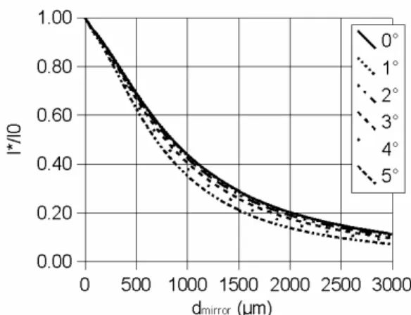
The analysis of Fig. 8 and Fig. 9 indicates that the measured intensity is highly dependent on the interface angle (φ). It also shows that the sensitivity of the measurement is reduced as the fiber core diameter is increased. On the other hand, it is possible to measure a thicker film thickness. According to Fig 8, the 50 µm core diameter fiber can measure a film thickness up to approximately 1.5 mm. However, with a 80 µm core diameter fiber, it is possible to measure film thickness up to approximately 2.5 mm (Fig. 9).

Figure 8. Theoretical results for optical fiber with 50 µµµµm core diameter, 0.2 numerical aperture, 5.28° beam emerging angle and i nterface angles from 0o to 5o.

Figure 9. Theoretical results for optical fiber with 80 µµµµm core diameter, 0.2 numerical aperture, 5.28° beam emerging angle and i nterface angles from 0o to 5o.

Figure 10. Theoretical result for optical fiber with 0.5 numerical aperture, 500 µµµµm core diameter and the emerging beam has 23.16°.

Results and Discussions

A simple experiment with a planar mirror was performed in order to verify the behavior described in the preceding section. The experimental results for the reflected laser intensify are shown in Fig. 11 and the intensity distribution in the emerging beam is shown in Fig. 12.

0 0,2 0,4 0,6 0,8 1 1,2

0 0,5 1 1,5 2 2,5 3

dmirror (mm)

(I

*-If

)/

I0

0° (exp.)

2° (exp.)

5° (exp.)

0° (theo.)

2° (theo.)

5° (theo.)

Figure 11. Results of planar mirror experiment and simulation with 500 µµµµm acrylic optical fiber and emerging beam with 23.16°.

Figure 12. Flux intensity profile of the laser beam in two distances from emitting lens.

The discrepancy between the theoretical and the measured intensity results, as shown in Fig. 11, can be explained by the characteristics of the acrylic optical fibers that have great internal attenuation when compared to glass optical fibers. Another significant problem is the fragility of this fiber that accumulates defects when manipulated. These internal defects contribute to the departure of measured intensity profile from the Gaussian distribution profile, as shown in Fig. 12. The internal failures also cause radiation leakage that can be observed by inspection of the optical fiber when it is conducting light radiation.

The calibration of the optical system was made using the test channel. The signal to thickness relation was obtained by adding discrete quantities of known water volume (no flow condition, wave generator stopped) in the channel and recording the signal in the computer. The curve obtained with this process was used to translate the data recorded in the experiment to film thickness.

The experiment was based on the variation of the film thickness and wave frequency. The channel was filled with a known volume of water that corresponded to an average thickness. Then a frequency was selected, the wave generator was switched on and the laser reflected signals were measured. The three different frequencies used in the experiments were determined afterwards by using the results. Two photographs were taken for each experimental run. Then, more water was added to the channel and additional data were taken for three frequencies as well as the respective photos. These measurements were done for three additional levels in order to verify the behavior of the technique under different frequency and film thickness variations.

The measured signals were filtered by the application of an averaging filter. The resulting curves were filtered again by an algorithm that identifies signal peaks that corresponds to interface wave peaks and valleys.

Due to its optical nature, the laser reflected intensity signal reaches a maximum value only when the interface wave is parallel to the tip of the optical fiber (maximum reflected intensity). This situation (interface parallel to the tip of optical fiber) only occurs when a wave peak or valley is passing in front of the tip of the optical fiber.

The filter used to find peaks and valleys takes the 25th sample of a set of 51 samples and verifies whether this is the maximum intensity of the set of data. It was chosen 51 samples because it was observed that there wasn’t more than one peak in 100 samples, taking a sample rate of 1000 samples per second. Then, the resulting filtered points were translated into thickness signal using the calibration curve.

J. of the Braz. Soc. of Mech. Sci. & Eng. Copyright  2006 by ABCM 35

1 1,5 2 2,5 3 3,5

1,5 2 2,5 3 3,5

Steady thickness (mm)

h

f

(m

m

)

From laser measurement From photographic data

Figure 13. Measured film thickness (average) compared with reference thickness taken from photographic data (average).

The measurements of interface wave velocity and frequency were made using the calculation of correlation coefficient between the two signals recorded from each oscilloscope channel (each channel connected to one optical fiber). After application of the averaging filter, the signals were used to calculate the interface wave velocity and frequency.

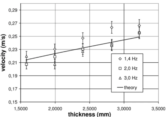
The wave velocity results for each average thickness can be observed in Fig. 15. The wave velocity was calculated by evaluating the correlation factor. Once the oscilloscope signal is an array of discrete points, by the introduction of a given delay between signals for a given interval of sample units and calculating the correlation, a given interval of time samples shall exist that maximize the value of correlation. By dividing the distance between the optical fibers by the obtained time interval, it was possible to calculate the wave velocity.

Figure 14. Picture taken from the place where the optical fiber were installed. The height of each optical fiber is 3 mm (from bottom of the channel to optical fiber tip).

The same can be done for frequency calculation, once the proposed wave generator creates a periodic disturbance in the gas-liquid interface. Then, the maximization for the correlation coefficient will be found twice, once for the delay between the signal passing through the two optical fibers and another for one entire wave period.

The theoretical values for velocity for each thickness can be obtained by the following equation (Moody, 1990):

0,15 0,17 0,19 0,21 0,23 0,25 0,27 0,29

1,5000 2,0000 2,5000 3,0000 3,5000

thickness (mm)

v

e

lo

c

it

y

(

m

/s

)

1,4 Hz 2,0 Hz 3,0 Hz theory

Figure 15. Wave velocity for each average thickness and frequency compared with theoretical data.

v= h⋅g (4)

where h is the film thickness and g is the local acceleration of gravity. The experimental wave velocity results were compared to the theoretical values and showed good agreement.

For the film thickness measurement, the uncertainties were evaluated by combining the uncertainties of the various measurement devices, including the Type A uncertainty of the oscilloscope signal. To calculate the expanded uncertainty, it was used a factor of two for 95% confidence level (two standard deviation). The expanded uncertainty for the film thickness measured by this technique was found to be 0.22 mm. The expanded uncertainty of the velocity was calculated by combining the uncertainty of the measurement devices and was found to be 0.01 m/s.

Conclusion

The objective of the present work was to develop a film thickness and velocity measurement technique using laser intensity measurement in liquid film flow. This work, which comprises both theoretical and experimental studies, was successfully conducted and provided important results.

The utilization of optical fibers with big core diameters increased the measurement range (up to 4 mm) and allowed great installation tolerances, when compared to small core diameter fibers. For this type of optical fiber the angular errors in installation are acceptable and do not cause any relevant effect on the quality of the measurements.

A theoretical model was proposed for the optical phenomena present in the film thickness measurement. The theoretical results of the model were compared to a simple experiment using a planar mirror. The overall calculation procedure was proved to be valid, although differences between theoretical and experimental results were found. These differences were caused by the use of acrylic fibers that introduced distortions in the beam intensity distribution. The acrylic optical fiber with 500 µm was less tolerant to manipulation, causing accumulation of damages in the fiber. These damages caused deviations in the intensity distribution of the beam that emerges from the optical fiber.

through the transparent channel walls, allowing the comparison to the results taken by the laser technique. The results show that the use of big core optical fibers can increase the measurement range up to 4 mm film thickness. The experimental results for the film thickness presented a good agreement with the reference thickness taken from photographic data. The interface wave propagation velocities presented small uncertainties and good agreement with the theoretical data.

References

Driscoll, D. I., Schmitt, R. L. and Stevenson, W. H., 1992, “Thin Flowing Liquid Film Thickness Measurement by Laser Induced Fluorescence”, Journal of Fluids Engineering, Vol. 114, pp. 107-112.

Fukano, T., 1998, “Measurement of time varying thickness of liquid film flowing with high speed gas flow by a constant electric current method (CECM)”, Nuclear Engineering and Design, Vol. 184, pp. 363-377.

Geraets, J. J. M. and Borst, J. C., 1988, “A Capacitance Sensor For Two-Phase Void Fraction Measurement and Flow Pattern Identification”, International Journal of Multiphase Flow, Vol. 14, 3, 305-320.

Hewitt, G. F., 1978, “Measurement of Two Phase Flow Parameters”, Academic Press, London.

Kamei, T. and Serizawa, A., 1998, “Measurement of 2-dimensional local instantaneous liquid film thickness around simulated nuclear fuel rod by ultrasonic transmission technique”, Nuclear Engineering and Design, Vol. 184, pp. 349-362.

Kang, H. C. and Kim, M. H., 1992, “The Development of a Flush-Wire Probe and Calibration Method for Measuring Liquid Film Thickness”, International Journal of Multiphase Flow, Vol. 18, 3, 423-437.

Koskie, J. E., Mudawar, I. and Tiederman, W. G., 1989, “Parallel-Wire Probes For Measurement of Thick Liquid Films”, International Journal of Multiphase Flow, Vol. 15, 4, 521-530.

Moody, F.J., 1990, “Introduction to Unsteady Thermofluid Mechanics”, John Wiley & Sons, San Jose.

Ohba, K., Tanaka, H., Kawakami, N. and Nagae, K., 1992, “Twin-fiber optic liquid film sensor for simultaneous measurement of local film thickness and velocity in two-phase annular flow”, Proceedings of the 6th

International Symposium on Applications of Laser Techniques to Fluid Mechanics, Lisbon, Portugal, pp. 39.1.1-39.1.6.

Samenfink, W., Elsaber, A., Witting, S. and Dullenkopf, K., 1996, “Internal Transport Mechanisms of Shear-Driven Liquid Films”, Proceedings of the 8th _{International Symposium on Applications of Laser}