Rev. bras. meteorol. vol.27 número3

PRELIMINARY WIND ANALYSIS REGARDING DIFFERENT SPEED RANGES IN THE CITY

OF LA PLATA, ARGENTINA

GUSTAVO RATTO

, ANDRÉS NICO

1

_{Centro de Investigaciones Ópticas (CIOp), La Plata, Argentina}

2

Nacional de La Plata Facultad de Ingeniería, Universidad, La Plata, Argentina

3

_{Centro Agrario El Chaparillo, Junta de Comunidades de Castilla La Mancha. Ciudad Real. Spain}

4

Fundación Parque Cientíico y Tecnológico de Albacete, Programa INCRECYT, Albacete, Spain

gustavratto@gmail.com,

Received February 2011 – Accepted December 2011

ABSTRACT

La Plata city (approximately 800 000 inhabitants) has intense trafic and industrial activity; nevertheless, the city has no governmental air monitoring network for air pollutants and winds have been scarcely studied. Wind observations provided here (covering 1998- 2007) belong to a weather station that was contrasted against the unique governmental site in the city area (the Airport). The present preliminary study analyses wind direction frequencies according to wind speeds and emphasizes wind patters within the irst hour after calm occurrences.

Results show that independently of the wind speed, wind direction frequency roses are in general similar to each other. Low wind speeds may occur most of the time (on average 58.2 %) and together with calm occurrences (on average 17.1% ) constitute an important factor for the accumulation of air pollutants. The proposed “outgoing of calm” wind direction frequency roses were found to be appropriate to gain knowledge in the structure of winds that transport pollutants towards exposed population after calm occurrences. Long term systematic meteorological ieldworks should be encouraged in the future so as to provide better tools for environmental modeling.

Keywords: calm analysis, La Plata, wind analysis, wind roses

RESUMO: ANÁLISE PRELIMINAR DO VENTO SEGUNDO DIFERENTES FAIXAS DE

VELOCIDADES NA CIDADE DE LA PLATA, ARGENTINA

A cidade de La Plata (aproximadamente 800.000 habitantes) tem tráfego e atividade industrial intensos. Contudo, não tem uma rede oicial de monitoramento para os contaminantes do ar e os ventos têm sido pouco estudados. As observações dos ventos aqui apresentadas (desde 1998 até 2007) correspondem a uma estação meteorológica que foi comparada com o único sitio oicial de registros de ventos na área urbana (o Aeroporto). O presente estudo preliminar analisa as frequências das direções do vento, segundo as suas velocidades, e coloca ênfase nos padrões de vento na primeira

hora após as ocorrências calmarias.

Os resultados mostram que as rosas de frequências de direções de ventos são em geral similares entre elas independentemente das velocidades. Velocidades baixas de ventos são factíveis de acontecer na maior parte do tempo (na média 58,2%), e, junto com as ocorrências de calmarias (na média 17,1%), constitui um fator importante para acumulação dos contaminantes. As rosas de frequência de direções de ventos propostas, nomeadas “saída de calmarias”, resultaram ser apropriadas para o conhecimento da estrutura dos ventos que transportam os contaminantes acumulados em direção à população exposta, após períodos de calmaria.Na meteorologia deveriam se incentivados os trabalhos de campo sistemáticos, de longo prazo, de forma a prover melhores ferramentas para a modelagem de meio ambiente.

1. INTRODUCTION

The city of La Plata is considered, along with its neighboring areas (approximately 800 000 inhabitants), one of the six most potentially hazardous cities in Argentina regarding air pollution (Petcheneshky et al., 1998). An industrial complex (see the rectangle in Figure 1) containing the country´s main oil reinery (total crude oil processing capacity of 32 000

m3/day), petrochemical plants, steel processing plants and a

shipyard along with heavy trafic activity (approximately 300 000 vehicles) (Whichmann et al., 2009) are the main sources of anthropogenic airborne pollutants. In addition, a new thermal power station (with a capacity of 560 MW) constructed in the vicinity areas of the industrial complex is due to be operating at the beginning of 2012. Besides the local burden of regional pollutants contributors, such as those belonging to biomass burning transported by low- level jets (Ulke et al., 2007; Ulke, 2009) should be taken into account in future studies. A recent study (Cataldi et al., 2010) points out the importance that regional anomalies (such as El Niño) may have in local

atmospheric circulation patterns.

Although the great need of a systematic air pollution assessment, the city has no governmental monitoring network. Several works evaluate different aspects of air pollution in the

area (Colombo et al., 1999; Rosato et al., 2001; Ronco et al., 2001; Massolo et al., 2002; Rehwagen et al., 2005; Nitiu, 2006, Massolo et al., 2010) but winds have been scarcely studied. In previous reports (Ratto et al., 2006, Ratto et al., 2009, Ratto et al., 2010a) the need of knowing wind patterns was pointed out in order to provide basis to air pollution modeling. Also some aspects of the boundary layer meteorology, such as the characterization of atmospheric stabilities and mixing depth (Mazzeo et al., 1971) and turbulence studies (Marañon Di Leo

et al., 2004) result scarce and incomplete up to date and should

be encouraged together with a wind proile analysis in order to provide basic tools to be applied in environmental modeling.

This article is intended as a preliminary work. Its purpose is to analyze the behavior of frequency wind roses regarding different speed ranges in order to gain knowledge of wind structure. Moreover wind patterns after calms are analyzed, taking into account that pollutants tend to accumulate within the areas neighboring sources during calm events (Alvarez Escudero et al., 2007). The irst winds after the calm would transport air masses with high charge of pollutants. Computing the irst wind direction that appears after a calm and accumulating this count for a given period allows the building up of a wind rose named “outgoing of calms wind rose” - OOC wind rose hereafter.

Seasonal OOC wind roses are presented and their relationship

with the averaged wind roses for different speed intervals are analyzed. As a consequence, wind directions relevant for the transport of air pollutant towards population exposed namely Sector 1 (NNW- NE) and Sector 2 (ENE- ESE) – see the bottom left corner of Figure 1- are discussed.

Overall comparisons between pairs of wind roses were carried out by applying the sum of the absolute values for the differences (SAD) between frequencies. This metric was used as

a dissimilarity criterion between wind roses but also provided a magnitude for the “error” of predicting outgoing of calms wind roses with the use of complete range wind roses. Measurements

involved correspond to one monitoring site located in a semi-

rural area (see Point J in Figure 1) that was in operation during 10 years. The observed data were seasonally grouped and compared to those of the La Plata Airport (see Point K in Figure 1) taken as reference.

2. MATERIALS AND METHODS

2.1 Area description and data characteristics

The city of La Plata is one of the most industrialized and populated cities within the La Plata River basin (3 200 000 km2_{) in central- eastern South America. The city is located close}

to the coast of the La Plata River (35º S 58º W) around 15 m above the sea level. Climate is temperate humid with an annual

Industrial Complex

K J

B C

3 km

Gonnet City Bell Villa Elisa

City Center Main Suburbs

Río de La Plata

Berisso Ensenada

Rural Area Rural Area

Rural Area

Punta Lara

N

E Sector 1

Sector 2

Figure 1 - Map covering parts of La Plata City and surroundings.

average temperature of 16 ºC and a medium annual rainfall of ca. 1000 mm (Negrin et al., 2007).

In the La Plata River region a considerable surface temperature contrast between water and land takes place setting the stage for the development of a low- level circulation with sea- land breeze characteristics (Berri et al., 2010). This

circulation makes the wind blows from water to land during the day (i.e. sea- breeze) and from land to water during the

night. Since this phenomena occurs in a lat terrain there are

no other topographical effects that inluence the low- level local circulation (Sraibman and Berri, 2009). This phenomenon

was evidenced during a short campaign in La Plata city when wind direction frequency roses at Point J were compared with observations at a weather station located close to the industrial complex (Ratto et al., 2010b).

The unique study found in the area of La Plata regarding atmospheric stability analyses (Mazzeo et al., 1971) covered the period 1957- 1966. It was carried out near the industrial complex and involved day- time hours. This study was based on Turner´s classiication where class A refers to an extremely unstable atmosphere, class B to unstable, class C to slightly unstable, class D to neutral, class E to slightly stable, class F stable and class G extremely stable. An overall view of stability classes on annual basis determined that class D was prevailing (49% of the time) followed by class E (20.8%) and class C (17.4 %). The same study shows that the average mixing height values (measured during 1965- 1968) for winter was about 700 m while for summer was about 1700 m.

Monitoring site Point J (see Figure 1) is located in a

semi- rural area around 18 km far from the river bank (labeled as C) and around 9 km far from La Plata Airport. Data belonging to Point J – Agrometeorological Station- National University of La Plata- cover the period 1998- 2007 and were obtained with a GroWeather® Industrial. (Davis Instruments Corp, San Francisco, US) meteorological station. Wind directions were obtained every 22.5° with an accuracy of ± 7° of the read out. The detection limit and resolution for wind velocities were 1.6 km h-1 _{and the accuracy ± 5 % of the read out. This station}

measured at 5 m above the ground and provided 16- direction wind roses. The data spanning from summer 1998 to spring 2007 was provided in hourly averages. Winter 2000 had insuficient data and was disregarded (no method of gap illing was applied). Nevertheless, this loss represented just 10% of the missing data within the complete set for winters. The rest of the missing data for winters and the rest of the seasons were distributed randomly throughout the 10 years. The completeness of data for winters was of 88.3 %; the completeness of the data for all the seasons was on average 93.4%. Previous to analyze how the observed seasonal frequency wind roses depend on wind speed, the wind speed structure was studied. As wind speeds provided by the

weather station at Point J were given in discrete intervals of 1.6 km h-1 _{the frequency for each of the discrete values was}

accumulated.

The reference site (Point K) is a weather station that belongs to the National Meteorological Service; it is located in a rural area and measures at 10 meters above the ground. The data set consisted of monthly averages for the decade 1991- 2000. This decade was selected because it was the closest one available to the observed data. Frequencies and speeds were given for 8 directions wind roses.

2.2 Statistical analysis

In order to make comparable 16 directions wind roses (as those observed for Point J) with 8 directions wind roses (those belonging to the reference site Point K) a classical approach was applied (Conrad and Pollak, 1950). This approach takes the 16 directions wind roses, keeps unvaried the main eight directions and assigns half of the frequencies of the secondary directions to each one of the adjacent respective principal directions. With this method the wind roses of Figure 2 were estimated.

The well known “sum for the absolute values of the differences” -SAD- is a metric that measures differences

between vectors by addressing the “distance” between them.

As the Euclidean distance, SAD is often employed to estimate

similarity. It is indeed a dissimilarity measure because as far as it grows the patterns involved are considered more different.

where i is the dimension (direction) of the pattern (wind rose) involved (n is 8 or 16), xi the frequency of the pattern (wind

rose) X in the direction i and yi the frequency of the pattern

(wind rose) Y in the direction i.

The irst direction after the calm was counted in order to build the OOC wind roses. Seasonal frequency OOC wind roses

were then built for the whole period under study.

3. RESULTS

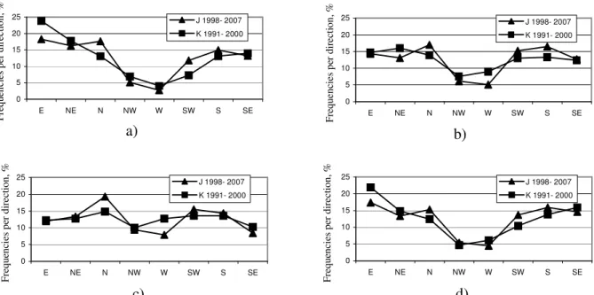
Reduced seasonal wind roses observed at Point J show, at irst sight, similar patterns to those corresponding to the reference site (Point K) for all seasons (Figure 2). Single absolute differences per direction between these wind roses were in all cases below 5.5 %. The similarity between sites involving wind frequencies is globally conirmed by obtained SAD values (Table

1). Seasonal averaged wind speeds at points J and K together with averaged calms are shown in Table 2. Observed wind speed average at Point J is 6.6 km h-1 _{while at Point K 18.9 km h}-1_.

Calm average at Point J is 17.1 % while at Point K is 24.2 %.

i i n

i y

x x y

SAD

SAD= =

∑

=1 ,

Frequencies corresponding to contiguous wind speeds for the data observed at Point J are shown in Figure 3. Up to 9.7 km h-1 _{differences between frequencies of contiguous wind}

speeds are for all the seasons below 3.1 %. For wind speeds above 11.3 km h-1 _{these differences are larger but occurrences}

are rarer. These two characteristics suggest that contiguous wind

speeds can be grouped into ranges; this step allows simplifying the subsequent analysis. Then, 4 speed ranges were built: 1.6- 3.2; 4.8- 6.4; 8.0- 9.6 and 11.3- 30.6 km h-1_{, also the complete}

range i.e. 1.6- 30.6 km h-1 _{is considered (Table 3, Figure 4).}

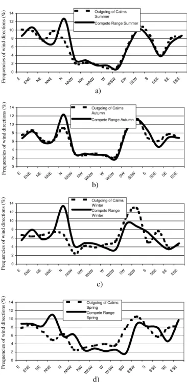
Figure 5 shows seasonal OOC wind roses together with

the corresponding complete range wind roses. Considering single directions the main differences are: 5.4 % for N and 2.9 % for NNE in Summer, 3.2 % for N and 1.7% for S in Autumn,

6.7 % for N and 4.1 % for SSW in Winter and 6.2 % for SW and 6.1 % for NNE in Spring. As a whole, major individual differences are all below 7%.

Estimated SAD between seasonal wind roses of Figure

4 and their corresponding OOC wind roses of Figure 5 (dash

line) are shown in Table 4.

In order to compare frequencies of sectors 1 and 2 corresponding to the complete range wind roses to those

corresponding to the OOC wind roses Table 5 was built.

The ratio between starting wind speeds for the irst hour after a calm involving complete range wind roses and OOC wind

roses are shown in Table 6.

4. DISCUSSION

The representativeness of meteorological data are user- dependent (Wieringa, 1996). Wind observations at airports- mainly devoted to help with plane trafic (Wieringa, 1980)- are not very appropriate for air pollution considerations (Holzworth, 1967). Nevertheless, due to scarcity of meteorological data in the

0 5 10 15 20 25

E NE N NW W SW S SE J 1998- 2007 K 1991- 2000

0 5 10 15 20 25

E NE N NW W SW S SE J 1998- 2007 K 1991- 2000

F

re

q

u

en

ci

es

p

er

d

ir

ect

io

n

,

%

0 5 10 15 20 25

E NE N NW W SW S SE J 1998- 2007 K 1991- 2000

F

re

qu

enc

ie

s

pe

r

di

re

ct

ion,

%

a)

F

re

q

u

en

ci

es

p

er

d

ir

ect

io

n

,

%

b)

c)

0 5 10 15 20 25

E NE N NW W SW S SE J 1998- 2007 K 1991- 2000

F

re

qu

enc

ie

s

pe

r

di

re

ct

ion,

%

d)

Figure 2 - Total frequency percentual wind roses at Point J and K. Seasonal wind roses belonging to Point J have been reduced from 16 to 8 directions

(Section 2.2) for the purpose of comparison with those at Point K (reference site). a) summer b) autumn c) winter and d) spring.

Table I

Summer Autumn Winter Spring

SAD _{21.8 17.5 15.5 17.9}

Table 1 - Seasonal SADa values for the wind roses of Figure 2.

Table II

Point J Point K

Summer Autumn Winter Spring Summer Autumn Winter Spring AWSa (km h-1) 6.9 6.4 6.7 6.2 19.2 17.7 18.5 20.1

Calmsb (%) 14.4 25.1 16.3 12.7 19.0 29.3 27.8 20.6

Table 2 - Observed and reference seasonal averaged wind speeds and calms

a _{Each SAD is computed taking into account the corresponding wind}

rose observed in points J and K

a _{Average wind speed}

area and in order to provide a context for the current analysis an overall comparison of observed and reference data is presented. Both sites show that N and NE are important winds for all the seasons followed by S (Figure 2). E and SE become more relevant in warm seasons while SW in cold ones.

Wind speeds at Point K are about three times higher than those at Point J (Table 2); this result can be attributed to friction forces that decrease with height as was evidenced by the anemometers located at 10 m (Point K) and 5 m (Point J) above the ground. Differences due to terrain roughness and data quality must be taken into account as well. For instance, measurements based on hourly winds carried out at 12 m above the ground in a urbanized area near the industrial complex during four years (Ratto et al., 2006) showed a general average of 9.4 km h-1_.

For the reasons explained above calms at Point K should be lower than those at Point J but calms at Point K are on average around 30% higher. This difference may be attributed to differences in data quality. Nevertheless note that both sites reveal the same trend (higher values in colder seasons than in warmer ones) being autumn the season with most of calm occurrences. Table 3 is intended to show how wind frequencies depend on wind speeds. It provides an overview of wind frequencies regarding the wind ranges previously deined. Low wind speeds

(below 6.4 km h-1_{) are more frequent in cold seasons (autumn}

and winter) than in warmer ones. On the other side, speeds above 8.0 km h-1 _{are more frequent in warmer than in colder seasons.}

Frequencies corresponding to speeds below 6.4 km h-1 _{(a very}

close value to those of any of the seasonal averages) represented

56.0 % in summer, 62.8 % in autumn, 59.5 % in winter and 54.6 % in spring (general average 58.2). Seasonal frequency wind roses for the ive speed ranges showed strong correlation within the seasons (Figure 4). Note that major differences were observed for N; the rest of the directions were very similar independently of the speed range.

As mentioned before the knowledge of wind patterns immediately after calms is important for air pollution modeling.

While SAD is a coeficient easy to compute, the computation of

the OOC wind roses as well as average wind roses for different

speed ranges is a time-consuming task, then it is desirable to know the degree in which OOC patterns can be “represented” by

any of the particular range patterns. In this sense, SAD provides

the degree for the “error”. According to this, wind roses that best

represent the OOC wind roses were that of the range 4.8- 6.4

for summer, that of the complete range for autumn, and that of the range 1.6- 3.2 for winter and spring (Table 4). Wind roses involving low wind speeds, i.e. range 1.6- 3.2 km h-1 _{and 4.8-}

Figure 3 - Wind frequencies (Y axis) for each of the wind speed step (X axis) supplied by the weather station at Point J. a) summer b)autumn c)

winter and d) spring.

7

0 4 8 12 16 20

1,63,24,86,48,09,7₁₁,3₁₂,9₁₄,5₁₆,1₁₇,7₁₉,3₂₀,9₂₂,5₂₄,1₂₅,7₂₇,3₂₈,9₃₀,6 0

4 8 12 16 20

1,63,24,8 6,48,09,7₁₁,3₁₂,9₁₄,5₁₆,1₁₇,7₁₉,3₂₀,9₂₂,5₂₄,1₂₅,7₂₇,3₂₈,9₃₀,6

0 4 8 12 16 20

1,63,24,86,48,09,7₁₁,3₁₂,9₁₄,5₁₆,1₁₇,7₁₉,3₂₀,9₂₂,5₂₄,1₂₅,7₂₇,3₂₈,9₃₀,6 0

4 8 12 16 20

1,63,2 4,86,48,0 9,7₁₁,3₁₂,9₁₄,5₁₆,1₁₇,7₁₉,3₂₀,9₂₂,5₂₄,1₂₅,7₂₇,3₂₈,9₃₀,6

a)

F

re

qu

en

ci

es

o

f

w

ind

spe

eds

(

%

)

b)

c)

d)

F

req

u

en

ci

es

o

f

w

in

d

s

p

eed

s

(%

)

F

re

qu

enc

ie

s

of

w

ind

spe

eds

(

%

)

F

re

qu

en

ci

es

o

f

w

ind

spe

eds

(

%

)

Wind speeds (km h-1_{) Wind speeds (km h}-1₎

Table III Wind speed range

(km h-1₎

Frequency (%)

Summer Autumn Winter Spring

1,6- 3,2 28,7 33,6 32,9 28,4

4,8- 6,4 27,3 29,2 26,6 26,2

8- 9,7 25,1 21,3 22,1 23,6

11,3- 30,6 18,9 15,9 18,3 21,9

Total 100 100 100 100

Table 3 - Observed frequencies for different speed ranges corresponding to Point J

0 2 4 6 8 10 12 14 E

ENE NE NNE N NN W _NW

WN W W

WSW SW SSW S

SSE SE ESE Outgoing of Calms

Summer

Compete Range Summer

0 2 4 6 8 10 12 14 E EN

E _NE NN

E N NN

W _NW WN

W W

WSW SW SSW S

SSE SE ESE Outgoing of Calms

Autumn

Compete Range Autumn

0 2 4 6 8 10 12 14 E ENE N

E

NNE N NNW NW WN W W

WSW SW SSW S

SSE SE ESE Outgoing of Calms

Winter Compete Range Winter 0 2 4 6 8 10 12 14 E

ENE NE NNE N NN W _NW

WN W W

WSW SW SSW S

SS E _SE

ES E Outgoing of Calms

Spring Compete Range Spring a) b) c) d) F re qu enc ie s o f w ind di re ct ions ( % ) F re qu enc ie s o f w ind di re ct ions ( % ) F re qu enc ie s o f w ind di re c ti ons ( % ) F re qu enc ie s o f w ind di re c ti ons ( % )

Figure 4 - Observed frequency wind roses at Point J according to

different wind speed ranges. In boded line is represented the wind rose involving all wind speeds (complete range). a) summer b) autumn c) winter and d) spring.

Figure 5 - Outgoing of calms and complete range wind roses at

Point J covering the period 1998- 2007. a) summer b) autumn c) winter d) spring.

0 5 10 15 20 25 30 E

ENE NE NNE N NN W

NW WN

W W

WS

W _{SW SS}W S

SSE SE ESE Range 1,6- 3,2 Range 4,8- 6,4 Range 8- 9,7 Range 11,6- 30,6 Complete Range 0 5 10 15 20 25 30 E ENE N

E

NNE N NNW NWWN

W W

WSW SW SSW S

SS E _SE

ES E Range 1,6- 3,2 Range 4,8- 6,4 Range 8- 9,7 Range 11,6- 30,6 Complete Range 0 5 10 15 20 25 30 E ENE N

E

NNE N NN W

NW WN

W W

WSW SW SSW S

SS E _SE

ES E Range 1,6- 3,2 Range 4,8- 6,4 Range 8- 9,7 Range 11,6- 30,6 Complete Range 0 5 10 15 20 25 30 E

ENE NE NN E N

NN W _NW

WN

W W

WSW SW SSW S

SSE SE ESE Range 1,6- 3,2 Range 4,8- 6,4 Range 8- 9,7 Range 11,6- 30,6 Complete Range a) F re qu enc ie s o f w in d di re c ti ons ( % ) b) c) d) F re qu en ci es o f w ind d ir ec ti ons ( % ) F re q u enc ie s o f w ind di re ct ion s (% ) F re qu enc ie s o f w ind di re c ti ons ( % )

a_{Each value of the table represents the percent of time that wind speeds (km h-1)}

belonging to one particular range were occurring.

6.4 km h-1 _{are on average more similar to the OOC wind rose}

than wind roses involving the rest of the ranges including those of complete range. This result is according to what is expected because winds immediately after calms are likely to have low speeds., For the case under study, the SAD allows infer that if

the complete range wind rose is used instead of the OOC wind

rose the “error” is around 22%.

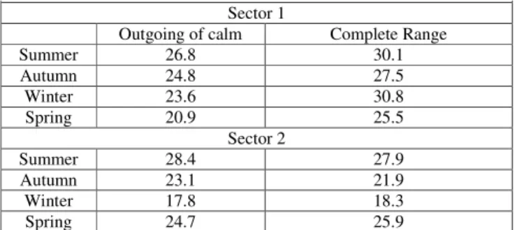
Sectors 1 and 2 are of interest regarding air pollution control (Ratto et al., 2009). Sector 1 involves winds that carry air pollutants towards city center and Sector 2 involves winds that carry pollutants towards the main residential areas (Gonnet, City Bell, etc.).

Comparing observed frequencies between OOC and complete range wind roses for both sectors major differences

appear in winter (maximal is 7.2%) for Sector 1. For Sector 2 all the differences are below 1.2% (Table 5). This implies that for these sectors the complete range wind rose predicts the outgoing of calms wind rose with a small error.

For all the directions of the compass but particularly for sectors 1 and 2 it is important to estimate the relationship between wind speeds regarding complete range and OOC wind roses. In

most cases, wind speeds involving both sectors are around 2.5- 3 times lower than those of the average wind speeds (Table 6). As mentioned before (Section 1) pollutants tend to accumulate during calm events but also large pollutant concentrations might occur under convective low wind conditions due to elevated point sources (Moore, 1969; Deadorff, 1984) such as those belonging to the petroleum processing plants. According to McCormick (1968), the persistence of surface wind less than 10 km h-1 _{is usually conductive to the}

accumulation of air pollutants. Sharan et al. (1996) and Goyal and Rama Krishna (2002) say that surface winds below 7.2 km

h-1 at 10 m level are considered as low wind speeds.

Applying to the well- known potential formulae to correct wind speed exposures (Seinield and Pandis, 2006) and considering site J as a rural place and neutral stability (see Section 2.1), the corrected value for 6.4 km h-1 _corresponds

to 7.1 km h-1_{. So considering the information given in Table}

3 (see frequencies for wind speeds

≤

≤

Table 2 and the average predominant role of the stability classes D and E (Mazzeo et al., 1971) most of the time the area has conditions that make dificult the removal of airborne pollutants. Regarding smoke plumes during winter nights -when stability class E together with low mixing heights (see Section 2.1) are more probable to occur- smoke plumes with “fanning” characteristics may develop (Stull, 1988) making dificult the vertical dispersion of air pollutants.

Knowledge on how frequent low wind speeds may occur in the area should be taken into account when applying Gaussian plume dispersion type models because (for low wind speeds) such models increase the error in the prediction of air quality pollutant concentrations as far as wind speeds decrease (Goyal and Rama Krishna, 2002).

Updated long fieldworks involving boundary layer regimes during daytime such as the Ulke and Mazzeo (1998)

Table V

Sector 1

Outgoing of calm Complete Range

Summer 26.8 30.1

Autumn 24.8 27.5

Winter 23.6 30.8

Spring 20.9 25.5

Sector 2

Summer 28.4 27.9

Autumn 23.1 21.9

Winter 17.8 18.3

Spring 24.7 25.9

Table 5 - Frequencies (%) for sectors 1 and 2 observed at Point J

corresponding to the wind roses of Figure 5.

Table VI

All directions Sector 1 Sector 2

Summer 2.5 2.5 2.3

Autumn 2.6 2.6 2.7

Winter 2.7 3.0 3.2

Spring 2.3 2.7 2.7

Average 2.5 2.8 2.6

Table 6 - Ratioa _{between wind speeds corresponding to complete range}

and outgoing of calm wind roses

Frequencies (percent of occurrences of winds) for Sectors 1 and 2 involving all the seasons from the point of view of the OOC and the complete range wind roses

a_{Ratio: average wind speed / outgoing of calms wind speed}

Column 2 indicates the ratio involving all directions of the compass, column 3 is the analogous but only for the directions of Sector 1, column 4 involves only the directions of Sector 2.

Table 4 - Frequencies (%) for sectors 1 and 2 observed at Point J corresponding to the wind roses of Figure 5.

Table IV

Compete Range 1.6- 30.6 km h

-1

Range 1.6- 3.2 km h-1

Range 4.8- 6.4 km h

-1

Range 8.0- 9.7 km h

-1

Range 11.6 – 30.6 km h

-1

Summer 16,9 18,7 13,2 28,4 49,4

Autumn 10,7 16,6 16,7 22,3 48,2

Winter 27,9 20,7 24,1 69,0 66,4

Spring 31,7 23,4 27,6 37,1 52,9

analysis for Buenos Aires City and the approaches suggested by Mahrt (1979) and Mahrt et al. (1998) for nighttime involving wind proiles, mixing heights and stability analyses as well as land- sea breeze studies (Tayt-Son et al., 2010) involving land- sea breeze front variations with time (Simpson, 2006) are of vital importance in order to deepen in the physical aspects of pollutant transport and inally to reinforce or correct the preliminary indings of this work.

Regarding pollution control, a medium term campaign

assessing basic meteorological parameters -such as wind direction frequencies, wind speeds, calms, minimum temperature, pressure and relative humidity- (Lalas et al., 1982) together with some primary industrial and power plant air pollutants (such as

SO2, PM10, NOx) will be very adequate to settle reference for

the air pollution status of La Plata area.

5. CONCLUSIONS

The study focuses on local observations but other scales (involving regional low- level jets and El Niño phenomena) should be considered in the future to provide an integrated and realistic overview of local processes.

Observed seasonal wind frequency patterns for the period under study were found very similar to those corresponding to La Plata Airport taken as reference. Wind speeds and calms did not keep such similarity but the differences can be explained in terms of exposure, terrain roughness and data quality.

Frequency wind roses for different speed ranges exhibited a very similar pattern. North direction showed major variations; it increases its frequency as far as averaged wind speed does.

Knowledge of winds after calms is very important in order to gain insight in wind characteristics. Wind direction frequencies considering only wind speeds during the irst hour after calms showed a very similar pattern to that of the complete speed range frequency pattern; for the case under study, the irst can be predicted by the latter with a small error.

Wind speeds after calms involving sectors 1 and 2 are signiicantly lower than their corresponding general averages for these sectors. This implies that not only calm events are of concern for the accumulation of air pollutants but also low wind speeds. La Plata city area needs long systematic ieldworks regarding meteorological aspects of air pollution transport, modeling and assessment. This will enrich the main indings of this preliminary study.

6. ACKNOWLEDGMENTS

The authors are grateful to the Experimental Station “Julio Hirschhorn” of La Plata National University for providing the data at Point J and to Dr. Christian Weber for his help. Our

particular thanks to Drs. Jorge Reyna Almandos and Fabián Videla for their contributions to this paper. We also appreciate very much the help of Dr. Alberto Lencina from CIOp.

7. REFERENCES

ALVÁREZ ESCUDERO, L.; ALVÁREZ MORALES, R.;

ROQUE RODRIGUEZ, A. Climatología del Viento y sus Aplicaciones II, 2007. Aplicaciones. En: Contribución

a la Educación y la Protección Ambiental. Cátedra de Medioambiente. Instituto Superior de Ciencias y Tecnologías Nucleares. p.5 Editorial Academia, La Habana, Cuba.

BERRI G.J.; SRAIBMAN, L.; TANCO, R.; BERTOSSA, G.

Low-level wind ield climatology over the La Plata River region obtained with a mesoscale atmospheric boundary layer model forced with local weather observations. Journal of Applied Meteorology and Climatology, 49, 6, 1293-

1305, 2010.

CATALDI, M.; FREITAS ASAD, L. P.; TORRES JUNIOR, A. R.; DRUMMOND ALVES, J. L. Estudo da inluência das anomalias da tsm do atlântico sul extratropical na região da conluência brasil malvinas no regime hidrometeorológico

de verão do sul e sudeste do Brasil. Revista Brasileira de Micrometeorologia 25: 513- 524, 2010.

COLOMBO, J. C.; LANDONI, P.; BILOS, C. Sources,

distribution and variability of airborne particles and hydrocarbons in La Plata area, Argentina. Environmental Pollution, 104: 305- 314, 1999.

CONRAD, V.; POLLAK, L. W.. Methods in climatology, 2nd Edition. 459 pp. Harvard university press, Cambridge, Massachusetts, 1950.

DEARDORFF, J.W. Upstream diffusion in the convective

boundary layer with weak or zero mean wind. In: FOURTH JOINT CONFERENCE ON APPLICATION OF AIR POLLUTION METEOROLOGY, 1984. American

Meteorological Society, Boston Massachusetts. Anais... 1984.

GOYAL, P.; RAMA KRISHNA, T.V.B.P.S. Dispersion of pollutants in convective low wind: a case study of Delhi.

Atmospheric Environment, 36 2071–2079, 2002.

HOLZWORTH, G.C., 1967 Mixing depths, wind speeds and air pollution potential for selected locations in the United

States. Journal of Applied Meteorology, 6: 1039- 1044

LALAS, D.P.; VEIRS, V.R.; KARRAS, G.; KALLOS, G. An

analysis of the SO2 concentration levels in Athens, Greece. Atmospheric Environment, 16: 531-544, 1982.

MAHRT, L. An Observational Study of the Structure of the nocturnal boundary layer. Boundary Layer Meteorology,

MAHRT, L.; SUN, J.; BLUMEN, W.; DELANY, T.; ONCLEY,

S. Nocturnal boundary layer regimes. Boundary Layer Meteorology, 88:255-278, 1998.

MARAÑON DI LEO, J.; DEL NERO, S.; RAGAINI, J. C.; SACCHETTO, V.; COLOSQUI, J.; COLMAN, J.; BOLDES, U.; SCARABINO, A.; ROSATO, M.; REYNA

ALMANDOS, J. Air Concentrations of SO2 and Wind

Turbulence near La Plata Petrochemical Pole (Argentina).

Latin American Applied Research, 34: 55- 58, 2004.

MASSOLO, L.; MÜLLER, A.; TUEROS, M.; REHWAGEN, M.; FRANK, U.; RONCO, A.; HERBARTH, O. Assessment

of Mutagenicity and Toxicity of Different-Size Fractions of Air particulates from La Plata, Argentina, and Leipzig, Germany. Environmental Toxicology, 17: 219- 231, 2002.

MASSOLO L.; REHWAGEN, M.; PORTA, A.; RONCO, A.; HERBARTH, O.; MUELLER, A. Indoor-outdoor

distribution and risk assessment of volatile organic compounds in the atmosphere of industrial and urban areas.

Environmental Toxicology,25: 339–349, 2010.

MAZZEO, N.; NICOLINI, M.; MOLEDO, L.; MICHELONI,

R. Condiciones de Estabilidad Atmosférica y Capacidad de Dilución Vertical de Contaminantes en la Ciudad de La Plata. AIDIS, Buenos Aires pp. 101- 114, 1971.

MCCORMICK, R. A. Air Pollution Climatology. In: Air Pollution (Stern, A.) Vol. 1 Chapter 9 Second Edition New

York Academic Press, New York, 1968.

MOORE, D.J. The distributions of surface concentrations of

sulphur dioxide emitted from tall chimneys. Transactions of the Royal Society, 265, 1969.

NEGRIN, M.; DEL PANNO, T.; RONCO, A. Study of bioaerosols and site inluence in the La Plata area (Argentina) using conventional and DNA (ingerprint) based methods

Aerobiologia, 23:249–258, 2007.

NITIU, D.S. Aeropalynologic analysis of La Plata City

(Argentina) during 3-year period. Aerobiologia, 22: 79-

87, 2006.

PETCHENESHKY, T.; GRAVAROTTO, M.C.; BENITEZ, R.; DE TITTO, E. Gestión de la Calidad de Aire Urbano-

Industrial. Situación del Monitoreo de la Calidad del Aire

(GEMS- AIRE) en la República Argentina. pp. 1- 12 Departamento de Salud Ambiental del Ministerio de Salud y Acción Social de La Nación, AIDIS, Buenos Aires, 1998.

RATTO, G.; VIDELA, F.; REYNA ALMANDOS, J.; MARONNA, R.; SCHINCA, D. Study of meteorological aspects and urban concentration of SO2 in atmospheric

environment of La Plata, Argentina. Environmental Monitoring and Assessment, 121: 327- 342, 2006.

RATTO, G.; VIDELA, F.; MARONNA, R. Analyzing SO2

concentrations and wind directions during a short monitoring campaign at a site far from the industrial pole of La Plata,

Argentina. Environmental Monitoring and Assessment,

149: 229- 240, 2009.

RATTO, G.; VIDELA, F.; MARONNA, R.; FLORES, A.; DE

PABLO, F. Air pollutant transport analysis based on hourly

winds in the city of La Plata and surroundings, Argentina.

Water, Air & Soil Pollution, 208: 243- 257, 2010a.

RATTO, G.; MARONNA, R.; BERRI, G. Analysis of wind

roses using hierarchical cluster and multidimensional

scaling analysis at La Plata, Argentina. Boundary Layer Meteorology, 137: 477- 492, 2010b.

REHWAGEN, M.; MÜLLER, A.; MASSOLO L.; HERBARTH, O.; RONCO, A. Polycyclic aromatic hydrocarbons associated with particles in ambient air from urban and industrial areas.

Science of the Total Environment, 348: 199– 210, 2005.

RONCO, A.; MÜLLER, A.; REHWAGEN, M.; MASSOLO, L.; TUEROS, M.; PORTA, A.; FRANCK, U.; HERBARTH, O. Inluence of industrial, trafic and domestic emissions in the air quality of La Plata (Argentina) and Leipzig (Germany) and the potential risk associated with respiratory diseases and allergies, 2001 Proceedings of II Mercosul Chemical Industry Congress and VII Brazilian Petrochemical

Congress, IBP 13001. Anais... Rio de Janeiro: IBP—

Brazilian Petroleum and Gas Institute, 2001.

ROSATO, M. E.; REYNA ALMANDOS, J.; RATTO, G.; FLORES, A.; SACCHETTO, V.: ROSATO, V. G.; RIPOLI, J.; ALBERINO, J. C.; RAGAINI, J. C. Mesure de SO2 à La

Plata, Argentine. Pollution Atmosphérique 169: 85- 98, 2001.

SEINFELD, J.H.; PANDIS, S.N.Atmospheric Chemistry and Physics. From Air Pollution to Climate Change. Second

Edition, John Wiley & Sons, New Jersey, 2006.

SHARAN, M.; KUMAR YADAV, A.; SINGH, M.P.; AGARWAL, P.; NIGAM, S. A mathematical model for the dispersion of air pollutants in low wind conditions.

Atmospheric Environment, 30: 1209- 1220, 1996. SIMPSON, J.E. Sea breeze and local wind. Cambridge

University Press, Cambridge, UK, 2006.

SRAIBMAN, L.; BERRI G.J. Low-level wind forecast over the La Plata River region with a mesoscale boundary layer model forced by regional operational forecasts Boundary Layer Meteorology, 130:407- 422, 2009.

STULL, R.B. An introduction to Boundary Layer Meteorology. Dordrecht: Kluwer Academic Press, The Netherlands, 1988.

Belem, Brazil Disponível em http://www.cbmet2010.com/ anais/artigos/477_19535.pdf. 2010.

ULKE, A. G. Aerosol characterization in Buenos Aires and relationships with transport patterns in South America.

Revista Brasileira de Micrometeorologia. Edição especial, 2009.

ULKE, A.; MAZZEO, N. Climatological aspects of the daytime mixing height in Buenos Aires City, Argentina.

Atmospheric Environment, 32:1615- 1622, 1998.

ULKE, A.G.; LONGO, K.M.; FREITAS, S. R.; HIERRO, R.F. Regional pollution due to biomass burning in South America.

Ciếncia e Natura 10, 201, 2007.

WHICHMANN, F.A.; MÜLLER, A.; BUSI, L.E.; CIANNI, N.; MASSOLO, L.; SCHLINK, U.; PORTA, A.; SLY, P.D. Increased asthma and respiratory symptoms in children exposed to petrochemical pollution. Journal of Allergy and Clinical Immunology, 123: 632- 638, 2009.

WIERINGA, J. Does representative wind information

exist? Journal of Wind Engineering & Industrial Aerodynamics, 65: 1- 12, 1996.

WIERINGA, J. Representativeness of Wind Observations at Airports, Bulletin of the American Meteorological Society,