Application of the Aventech AIMMS20AQ airborne probe for turbulence measurements during the Convective Storm Initiation Project

(1)

ACPD

7, 3519–3555, 2007

Turbulence measurements using

the Aventech AIMMS20AQ

K. M. Beswick et al.

Title Page

Abstract Introduction

Conclusions References

Tables Figures

◭ ◮

Back Close

Full Screen / Esc

Printer-friendly Version

Interactive Discussion

Atmos. Chem. Phys. Discuss., 7, 3519–3555, 2007 www.atmos-chem-phys-discuss.net/7/3519/2007/ © Author(s) 2007. This work is licensed

under a Creative Commons License.

Atmospheric Chemistry and Physics Discussions

Application of the Aventech AIMMS20AQ

airborne probe for turbulence

measurements during the Convective

Storm Initiation Project

K. M. Beswick1, M. W. Gallagher1, A. R. Webb1, E. G. Norton1, and F. Perry2

1

School of Earth, Atmosphere and Environmental Sciences, University of Manchester, UK

2

School of Earth and Environment, University of Leeds, UK

Received: 13 November 2006 – Accepted: 11 January – Published: 7 March 2007 Correspondence to: K. M. Beswick (karl.beswick@manchester.ac.uk)

(2)

ACPD

7, 3519–3555, 2007

Title Page

Tables Figures

◭ ◮

Back Close

Full Screen / Esc

Abstract

The Convective Storm Initiation Project (CSIP) took place during the summers of 2004 and 2005, centred on the research radar at Chilbolton, UK. Precursors to convective precipitation were studied, using a comprehensive and broad-based range of fieldwork and modelling. The principal aim of CSIP was the detection of the primary and

sec-5

ondary initiation of convective cells. The Universities Facility for Atmospheric Measure-ments (UFAM) Cessna 182 was used to map temperature and humidity fields over a broad area within and beyond the Chilbolton radar beam. Additionally, air motion was measured using a new turbulence probe, the AIMMS20AQ. The performance of the probe is critically appraised, based on calibrations, test flights and data flights flown

10

during CSIP intensive operating periods. In general, the probe performed well, al-though some aspects require more careful data interpretation which we describe in detail.

1 Introduction

With the expected increase in the frequency, magnitude and e_ffects of extreme weather

15

events due to global warming (IPCC, 2001; Senior et al., 2002; McBean, 2004), it has become crucial for governments to be able to plan for both the short and long-term consequences of these events. In particular, there is a pressing need to issue suitable and timely warnings where imminent danger to population and infrastructure is expected.

20

The Convective Storm Initiation Project (CSIP) was set up to improve the spatial and temporal accuracy of forecasting of high precipitation events. Since the accuracy of existing forecasts was greatly dependent on the success of the forecast of the initial storm development, CSIP targeted the main mechanisms thought to be precursors of convective storms. Prior to CSIP, the scale of the measurements required to provide

25

(3)

ACPD

7, 3519–3555, 2007

Title Page

Tables Figures

◭ ◮

Back Close

Full Screen / Esc

studies focussing on the initiation of precipitating convection in the UK. The recently established NERC Centre for Atmospheric Sciences UFAM facility (Universities Facility for Atmospheric Measurement) allowed a comprehensive, broad-based approach, cov-ering all stages of storm development, including cases where convection was expected but failed to produce precipitation.

5

We report in this paper airborne measurements of wind and turbulence structure using the UFAM Cessna 182J during the CSIP programme. The measurements were made using a new fast-response probe, the AIMMS20AQ (manufactured by Aventech of Barrie, Ontario). We present two contrasting case studies of wind fields, and include an assessment of the performance of the instrument based on comparisons with a

10

ground-based wind profiler and network of automatic weather stations.

2 CSIP methodology

Fieldwork for CSIP consisted of a pilot project in June 2004, followed by a full intensive campaign from June to August 2005, with the pilot project being used to inform and optimise the use of equipment during the main campaign.

15

The work was centred around the Council for the Central Laboratory of the Re-search Councils (CCLRC) site at Chilbolton, on the eastern edge of Salisbury Plain (Goddard et al., 1994; Naud et al., 2005). The two primary instruments mounted on the 25 m radar dish at this site are the Chilbolton Advanced Meteorological Radar An-tenna (CAMRA), which can identify boundary-layer structures such as thermals and

20

cloud shapes, and also give wind and moisture fields, and ACROBAT – the Advanced Clear Air Radar for Observing the Boundary Layer and Troposphere. For CSIP, the radar measurements were supplemented with a UHF wind profiler, sodars and Doppler Lidars stationed at sites within the radar range, as well as a mesonet of automatic weather stations spaced at roughly 20 km intervals. Radiosondes were launched at up

25

to hourly intervals from six sites. The UFAM Cessna and the Institut f ¨ur Meteorologie und Klimaforschung (IMK) Dornier 128 were flown during selected conditions. CSIP

(4)

ACPD

7, 3519–3555, 2007

Title Page

Tables Figures

◭ ◮

Back Close

Full Screen / Esc

data from these instruments will be presented elsewhere, and an overview of the CSIP project is given by Browning et al. (2006) who also give details of the forecasting and modelling products used.

On any given day, the probability of the onset of convective precipitation was as-sessed by the use of the model early in the day, with a forecast available by 09:00 GMT.

5

If suitable conditions were forecast, then the day would be declared an Intensive Op-erating Period (IOP). The forecast was then used to determine the optimum flight plan for the Cessna and Dornier aircraft.

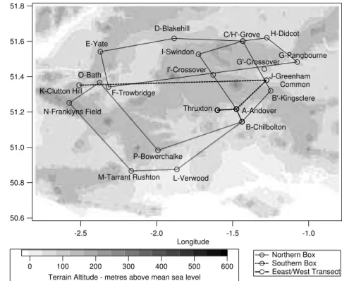
Three pre-determined flight paths were used, based on the set of navigational “way-points” shown in Fig. 1, giving a consistent dataset which would enable direct

compar-10

isons between flights. The first route was a simple East-West transit across Salisbury Plain between Greenham Common (waypoint J) and Bath (O). The second was the “Northern Box”, extending the East-West transit to the North using di_fferent combina-tions of waypoints depending on condicombina-tions. The third flight path was the ”Southern Box” with a loop down to the south coast before heading up to Bath, mainly flown by

15

the IMK Dornier. A fourth path was flown on the last day of the main project, with a North-South transit between Chilbolton and Swindon flown several times. Ideally, all flight paths were to be flown at a constant altitude of 2000 feet (610 m), with ad-justments for individual flights made according to air tra_ffic control instructions or local weather conditions.

20

A total of 18 IOP days were declared for the full CSIP campaign in 2005. The Cessna flew single flights on four of these days and two flights on three others: Table 1 lists the flights, indicating the routes flown.

3 Cessna instrumentation

The UFAM Cessna 182 J is a single-engine, high-winged aircraft, capable of flying at

25

an altitude up to 3000 m, with an endurance of around 4 h. The normal cruising speed

(5)

ACPD

7, 3519–3555, 2007

Title Page

Tables Figures

◭ ◮

Back Close

Full Screen / Esc

a payload of up to 130 kg. The aircraft has been owned and run by the University of Manchester since 1984 and has been used on a wide variety of research work e.g. Smith et al. (1989), Gallagher et al. (1990, 1994), Wood et al. (1999), Bower et al. (2000) and Webb et al. (2004). Although normally hangared at Liverpool John Lennon Airport, for the duration of the CSIP campaign the aircraft was kept at

Thrux-5

ton Airfield, in the centre of the CSIP operational area allowing a quick response to changing conditions.

The principal measurements for CSIP were position, temperature, humidity and air motion. The Cessna has a range of standard instruments for pressure, air speed and navigation, and these are supplemented by a suite of scientific instruments.

10

Air temperature was measured by three separate probes. The primary instrument was a constant current platinum wire total temperature probe in a wing-mounted Rose-mount inlet. The response time for this sensor was approximately 1 s (Wood, 1997). A second temperature sensor was mounted in a reverse-flow housing, allowing it to op-erate in wet and dry conditions. A second reverse-flow thermometer housed within the

15

AIMMS turbulence probe is detailed in Sect. 5. All temperature data were corrected for

dynamic heating effects (Lenschow, 1986) using recovery factors determined

specifi-cally for the Cessna instruments (Wood et al., 1997).

Absolute and relative humidity were derived from the Rosemount temperature and the dewpoint signal from a Michell S3000 Hygrometer. The response time as

deter-20

mined from spectral analysis of field data was 5 s (Wood, 1997). The AIMMS relative humidity sensor is discussed in Sect. 5 (response 1 Hz, Private communication, Bruce Woodcock, Aventech).

A Javad Navigation Systems AT4 di_fferential GPS (DGPS) system was used to

de-termine position at 10 Hz (the current equivalent model is the JNSGyro-4T). The AT4

25

uses four geodetic quality antennae arranged in a cruciform on the tail, wings and cabin roof, with a baseline of 5.3 m between the wing antennae. The antennae are capable of tracking up to 20 satellites each, and use the dual frequency (1565–1615 MHz and 1217–1265 MHz) carrier-phase method to greatly enhance the accuracy of the

(6)

ACPD

7, 3519–3555, 2007

Title Page

Tables Figures

◭ ◮

Back Close

Full Screen / Esc

surements. As well as providing accurate position, by calibrating the antennae on the ground over a period of around an hour, the positions of the antennae are known to an accuracy of around 1 mm relative to each other in three dimensions. By defining the tail antenna as the ”master” and the other three antennae as “slaves”, the AT4 can then calculate aircraft attitude angles (pitch, roll and heading) to an accuracy of

5

0.1◦_{, and position in three dimensions to within 0.01 m. This system is also used on}

the UFAM BAe 146 aircraft. For the Cessna application, the AT4 uses the standard NMEA $GPRMC command (DePriest, worldwide web) to output position, ground track and ground speed, as well as satellite time. Additionally, the three attitude angles are output via a command unique to the AT4.

10

The two wing antennae for the AT4 are shared with the GPS module which forms part of the AIMMS probe (see Sect. 5). Whilst altitude is available from the two GPS systems, this only gives height above the GPS geoid, not above sea level. Thus, for the purposes of this paper, altitude is calculated from the aircraft static pressure signal. All signals were logged to a custom-built PC-based logging system, comprising two

15

PCs running Windows XP, a 32 channel di_fferential A-to-D interface and an Amplicon

8-port serial card. The standard aircraft instruments and the AT4 were logged using custom-written LabView programmes, whilst the AIMMS was logged using software supplied with the probe.

4 Air velocity measurements from aircraft platforms

20

4.1 Theory

The true wind velocityV of atmospheric air relative to the surface of the Earth is found from the following vector sum:

(7)

ACPD

7, 3519–3555, 2007

Title Page

Tables Figures

◭ ◮

Back Close

Full Screen / Esc

where Va is the air velocity relative to the moving aircraft, and Vp is the velocity of

the aircraft with respect to the Earth. Thus V is the di_fference between two large

quantities and it is therefore essential that Va and Vp are measured as accurately

as possible in order to give an acceptable level of error in V, usually of the order of

0.5–1.0 ms−1 _{for meteorological research. Additionally, in order to be able to study}

5

small-scale structures, the frequency at which these quantities are measured must be suitable relative to the speed of the aircraft.

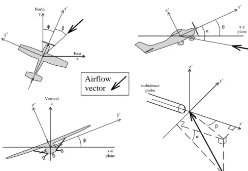
Equation (1) requires Va and Vp to be expressed in the same coordinate system.

Vpis defined relative to the Earth by three attitude angles, pitchθ, rollφand heading ψ, as shown in Fig. 2. The Earth coordinate axes are x,y and z, (collectively known

10

asS) wherex is positive in the East direction,y is positive in the North direction, and

z is positive in the upwards vertical direction. Va is measured relative to the aircraft

in thex′_y′_z′_{coordinate system (collectively known as}_S′_{), where}_x′_{is the longitudinal}

axis of the aircraft,y′_{is the lateral axis, and}_z′_{is the vertical axis, and is defined by two}

angles: vertical angle of attack,α; horizontal sideslip angle,β. Va must therefore be

15

mapped fromS′_to_S _{to allow Eq. (1) to be calculated.}

Figure 2 shows the relationship between theS andS′_{coordinate systems. A matrix,}

M_S′_→_S, is used to mapS′toS:

cosθsinΨ −sinφsinθsinΨ−cosφcosΨ −cosφsinθsinΨ +sinφcosΨ

M_S′_→_S=cosθcosΨ −sinφsinθcosΨ +cosφsinΨ −cosφsinθcosΨ−sinφsinΨ

20

sinθ sinφcosθ cosφcosθ (2)

The three rows ofM_S′_→_S transform the longitudinal, lateral and vertical components of

Va. The vector components of Va and Vp can then be used in Eq. (1) to give the air

motion vector in terms of north, east and vertical components. A full derivation of the transform matrix shown in Eq. (2) can be found in Wood (1997).

25

(8)

ACPD

7, 3519–3555, 2007

Title Page

Tables Figures

◭ ◮

Back Close

Full Screen / Esc

4.2 Turbulence probes

The most obvious di_fficulty in measuring air turbulence from any moving object is the removal of the platform velocity vector. Measuring turbulence from a fast-moving air-craft platform adds the further problem of removing significant airflow distortion induced by the aircraft itself. Combined with the need to measure the data as fast as possible

5

in order to improve spatial resolution, it is only recently that technology has been able to overcome these problems satisfactorily.

A number of systems have been developed over the years. Although successful measurements are possible using a simple 3-axis accelerometer system to determine the response of the aircraft to gusts of wind (e.g. Stromberg et al., 1989), this can be

10

subject to large errors due to the mass of the aircraft damping the response to turbu-lence. Notess et al. (1954) coupled accelerometers with fixed wind vanes and a pitot-static aircraft true air speed (TAS) sensor, whilst Telford and Warner (1962) improved on this system with the introduction of the gyro-stabilised platform, still a major compo-nent of modern inertial navigation systems. Whilst fixed and rotating vanes (Johnson et

15

al., 1978; Lenschow, 1971) have been used to measure airflow relative to the aircraft, it is now more common to use a di_fferential pressure method e.g. Brown et al. (1983), this being more reliable particularly under icing conditions. Typically, a “five-hole” ar-rangement of pressure ports is used, such as that in the Rosemount AJ858 gust probe (e.g. Bange et al., 2002). A more advanced instrument is the BAT Probe (Hacker and

20

Crawford, 1999) using a nine hole pressure port formation in conjunction with di_ff eren-tial GPS and fast-response accelerometers to give wind vector measurements at up to 50 Hz. Whiteway et al. (2003) used this probe to study breaking gravity waves at the top of the tropopause.

A five-hole turbulence probe was developed for use on the instrumented Cessna

25

182J (Wood et al. 1997), and the AIMMS turbulence probe, described in detail below, is based on the same principles, but incorporates state-of-the-art technology

(9)

ACPD

7, 3519–3555, 2007

Title Page

Tables Figures

◭ ◮

Back Close

Full Screen / Esc

computing power to allow the use of the Kalman Filter signal processing method.

5 The AIMMS20AQ probe

5.1 Technical description

The AIMMS20AQ probe – Aircraft Integrated Meteorological Measuring System 20Hz – was developed from wind sensors used in a crop spraying application designed to

5

help farmers meet regulations on pesticide application in the United States. In conse-quence, economies of scale ensure the probe is robust, reliable, relatively low cost and easy to install and calibrate. Whilst the Cessna uses the standard probe casing, the sensor head can also be supplied to fit a PMS pod to make it simple to fit on research aircraft which are already modified for this widely used type of canister.

10

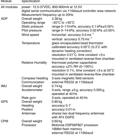
The AIMMS is essentially an up-to-date five hole probe, with all elements of the sen-sor, data processing and analysis in a stand-alone package. The system consists of four modules which will be described further below: ADP – the air data probe, compris-ing a five-hole pressure port head, and built-in temperature and humidity sensors; GPS – global positioning system linked to antennae on each wing; IMU – inertial

measure-15

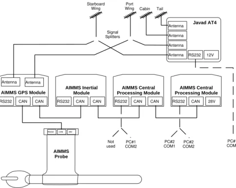
ment unit; CPM – central processing module. The modules are linked by a high-speed digital serial link known as the CAN – Controller Area Network – which also carries power between the modules. Figure 3 shows a schematic of the modules, and the technical specifications are given in Table 2.

The ADP has a cruciform array of five pitot-static pressure ports situated on a

hemi-20

spherical head which sits at the front end of a cylinder which also contains a ring of static pressure ports for determining aircraft TAS. The horizontal and vertical pairs detect sideslip angle and angle of attack respectively. The rear of the cylinder con-tains a reverse-flow housing for the temperature and humidity sensors. The cylinder is mounted below an aerofoil-shaped pylon which contains the transducer electronics.

25

The ADP can be mounted onto a wing strut or, in the case of the Cessna, directly to

(10)

ACPD

7, 3519–3555, 2007

Title Page

Tables Figures

◭ ◮

Back Close

Full Screen / Esc

the underside of the wing. The combination of the pylon and cylinder structure ensures that the pressure sensor sits upwind of, and below, the front edge of the wing, away from the influence of much of the induced airflow distortion. Weighing 3.6 kg and with a drag of 4.6 N at 50 ms−1_{, the probe has little e}

ffect on aircraft performance.

Com-bined with using fixing points on the Cessna wing originally used for a PMS canister,

5

this simplified the installation of the new probe. The PMS (Particle Measuring Sys-tems) canister has been a widely used method for mounting research instruments on aircraft for many years, making the modification process much simpler, both practically and in terms of meeting UK CAA and the European EASA regulations (CAA certificate number 9/218/M/5438 for this application).

10

The remaining three modules are mounted within the aircraft. As with the AT4 DGPS,

the AIMMS GPS uses the carrier-phase method to give accuracy of 0.1◦_{in the heading}

calculation. Only two antennae are required, and the wing antennae used for the AT4 are shared via signal splitters (GPS Networking Inc., Model LDCBS1X2).

Ideally, the IMU should be mounted as close to the centre of mass (CoM) of the

15

aircraft as possible, and preferably on the aircraft’s longitudinal axis. This ensures that the accelerometer signals are representative of the movement of the entire aircraft and are not due to rotation about the CoM or excessive flexing of the airframe. In the Cessna, the IMU is mounted on the longitudinal axis, but is located 3 m aft of the CoM. The IMU consists of a 3-axis accelerometer unit and a 3-axis system of rate

20

gyroscopes, both running at 40 Hz. Combining the signals from the IMU and GPS, the full attitude and motion of the aircraft can be determined at a rate of up to 20 Hz.

The CPM comprises a Motorola DSP56F807 processor with a 16Mbit internal flash memory. Using the CAN, data is taken from the ADP, IMU and GPS modules and pro-cessed. There are two mutually exclusive data recording methods. The first – raw data

25

(11)

ACPD

7, 3519–3555, 2007

Title Page

Tables Figures

◭ ◮

Back Close

Full Screen / Esc

have been carried out. The second method uses the calibration coefficients to give on-line wind speed data at up to 5 Hz: this relies on the magnetic and airflow calibrations being available in order to give a reliable solution, since the data cannot be further pro-cessed. The data is stored on the CPM flash memory and then extracted at the end of a flight as a CSV ASCII file. In both cases, an Extended Kalman Filter is used (Kalman,

5

1960; Welch and Bishop, 2004), in which a running average of an estimate of the error in the wind solution is used to prevent the integrated accelerometer signal from drifting. The Kalman filter requires a “spin-up” period of around 2 s in order to operate correctly, requiring the signals from the IMU and GPS to be bu_ffered in order to give an accurate wind vector solution.

10

The CPM communicates with an external computer via two RS232 ports at 156 kbaud. A configuration and logging program is supplied with the probe which allows the user to input calibration coe_fficients, decide which of the two serial ports is to be used, and to set the logging method to either on-line or raw data capture.

5.2 Calibration procedures

15

The AIMMS probe requires three separate calibrations, namely magnetic, aerodynamic and cross-axis. The on-line processing method requires that the magnetic and aero-dynamic calibrations have been carried out, although reliable data is then restricted to straight and level flight. For fully processed data, giving accurate wind speeds in most conditions, all three calibrations are essential. For all three calibrations, the data are

20

analysed by Aventech who then provide calibration coefficients.

The magnetic calibration is carried out on the ground. The aircraft is pointed to

magnetic north and then makes a 360◦ _{turn at a steady rate over a period of two}

minutes. The resulting calibration coefficients are then programmed into the CPM. The aerodynamic calibration is designed to quantify the e_ffect of distortion of the

25

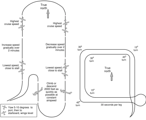
airflow around the aircraft when flying in a straight line, and must be carried out in the air, in conditions of uniform and low wind speed. Two pilot-induced manoeuvres are carried out, shown schematically in Fig. 4a. Firstly the aircraft is “yawed” 10◦_{, initially to}

(12)

ACPD

7, 3519–3555, 2007

Title Page

Tables Figures

◭ ◮

Back Close

Full Screen / Esc

the port side and then to the starboard side. This entails changing the aircraft heading whilst keeping the wings level, a procedure known as a flat turn. This is repeated at two di_fferent speeds (close to stall speed, and highest cruising speed) and in two reciprocal directions. This allows the probe’s response to sideslip angle to be calculated, whilst

removing the effect of the prevailing wind conditions. In the second manoeuvre, the

5

aircraft is made to climb 2000 feet rapidly at constant speed before making a 180◦_turn

and descending rapidly by 2000 feet. This allows the response to angle of attack to be quantified, again removing the effect of the prevailing wind.

The cross-axis calibration is again carried out in flight during calm and consistent conditions, and quantifies the response of the probe when the aircraft makes turns.

10

A square box is flown in clockwise and anti-clockwise directions, with banked turns of di_fferent roll angle at each corner, as shown schematically in Fig. 4b.

5.3 Quality control

At the time of the CSIP campaign for which these results are reported, the cross-axis calibration had not been completed for the AIMMS20, and the aerodynamic calibration

15

was not completed until after Flight 5. As a result, only data recorded during straight and level runs have been used. All data for flights 1 to 5 were made using the raw data mode but, for operational reasons, it was decided to use the on-line mode at 5Hz for subsequent flights, although full spectral analysis of the turbulence data would not be possible.

20

(13)

ACPD

7, 3519–3555, 2007

Title Page

Tables Figures

◭ ◮

Back Close

Full Screen / Esc

5.4 Data processing

In terms of importance for the CSIP campaign, the most useful output was for temper-ature, humidity and wind vector as a function of position along a given flight track. For the purposes of this paper, only the wind field data will be discussed in detail, where the data from the main loggers were averaged to 30 seconds. Additionally, in order to

5

characterise the abilities of the probe, the original on-line processed 5 Hz data were used for the AIMMS probe.

The AIMMS was logged to one of the on-board PCs, with the ASCII data processed through the proprietary programmes Microsoft Excel and Wavemetrics Igor Pro. The second PC was used to log all other data: the Javad AT4 was logged at 10 Hz via one of

10

the standard serial ports; the remaining signals were logged via a 32 channel A/D card. The A/D was logged at 20 Hz in binary format, although a separate 1 Hz ASCII text file was also written. This text file incorporated data processed to 1 Hz from the AT4 output, and allowed the data to be looked at with a minimal amount of processing at the end of a flight. Once again, Excel and Igor Pro were used for data processing and analysis.

15

Since the AIMMS data was logged independently, the datasets are synchronised by reference to the GPS satellite times recorded by the AIMMS and AT4, which should be consistent for the two instruments.

When analysing data as a function of position, an averaging period of 30 s was used (equivalent to a spatial resolution of around 1.7 km at a typical cruise speed of

20

55 m s−1_{), enabling large-scale features to be readily identified. This data was overlaid}

on terrain relief information taken from the US Geological Survey global 30 arc-second digital elevation model (GTOPO30), giving a spatial resolution of 1 km. The horizontal wind vector from the AIMMS was displayed along with data from ground-based instru-ments, including the UFAM wind profiler, and the University of Leeds AWS mesonet.

25

In terms of comparing air turbulence between different flights and flight legs, the variances of the horizontal and vertical wind components,σ2_w and σ2_{f f}, were of most

use, along with the turbulent kinetic energy (TKE). Here, _ff is the magnitude of the

(14)

ACPD

7, 3519–3555, 2007

Title Page

Tables Figures

◭ ◮

Back Close

Full Screen / Esc

horizontal wind calculated from the east (u) and north (v) components.

In order to determine whether the AIMMS was sampling all the scales of air motion, power spectral densities were computed for the wind components. When the power

spectrum is plotted on log-log axes, a gradient of –5/₃ should be expected across a

broad range of frequencies known as the inertial sub-range (Leslie, 1973), indicating

5

that all scales of turbulence are being sampled adequately.

5.5 Performance and characterisation

It is always necessary when using a new instrument to determine the quality of the data, to ensure that the installation optimises the performance of the probe. A test flight from Liverpool airport and CSIP Flight 8 on 19 August (see Table 1) have been used

10

to compare the position and attitude data with that obtained from the high precision Javad AT4. The ability to correctly map out a wind field was also examined, with Flight 8 being chosen as a day with a consistent wind flow across the CSIP area, allowing a comparison with ground-based instruments.

5.5.1 Comparison with the Javad AT4

15

A test flight was carried out from Liverpool airport in January 2006 which contained a number of tight manoeuvres under the direction of air tra_ffic control. This o_ffered an ideal opportunity to use the data to compare the performance of the AIMMS DGPS with the AT4.

It was assumed that the two systems reported position instantaneously since these

20

measurements require minimal processing. On this basis, the AIMMS reports heading, pitch and roll up to 2 s after the AT4, as expected due to the use of the Kalman filter processing method in the AIMMS data (see Sect. 5.1). Taking these time lags into account, the signals for position (i.e. latitude and longitude), heading, pitch and roll were then compared. The regressions for these comparisons are shown in Table 3.

25

(15)

ACPD

7, 3519–3555, 2007

Title Page

Tables Figures

◭ ◮

Back Close

Full Screen / Esc

is not as good, mainly due to discrepancies in magnitude. Further 5 Hz data from Flight 8 show that, unlike in straight and level flight, the time lag between the AIMMS and AT4 reduces in tight manoeuvres. This may reflect the capability of the AIMMS to measure attitude at 40 Hz, with the phase di_fference decreasing at higher rates of change of pitch: in effect the AT4 reacts less quickly to rapid changes in attitude than

5

the AIMMS. The relatively large o_ffsets in the pitch and roll regressions are due to the

AT4 calibration using a di_fferent baseline to the AIMMS, having been calibrated with

the aircraft stationary on the ground.

5.5.2 CSIP Flight 8 – uniform wind field

Flight 8, during IOP17 on 19 August, used the northern box route, flying the circuit

10

twice (see Table 1). This flight was chosen because the conditions on the day showed a moderate and consistent wind speed across the CSIP flying area. Developing cloud heads led to prolonged rain over the eastern half of the CSIP area and flash floods near the south coast in the morning, delaying the start of the IOP. During the early afternoon scattered showers broke out in Wales and the north-west midlands, followed

15

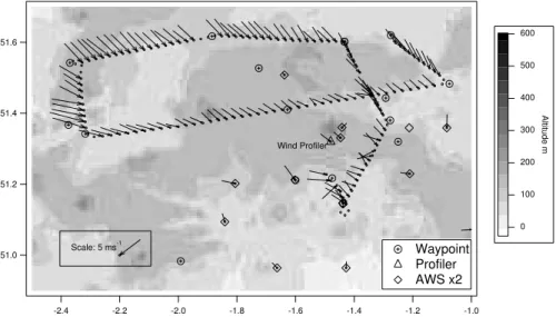
by the formation of a line of showers just west of Bath from 13:45 UTC. These showers reached peak intensity at 15:00 UTC with tops at 6 km, weakening between 16:00– 17:00 UTC, by which time the showers extended from east of Bath to the Isle of Wight. Figure 5 shows the wind speed and direction from the AIMMS as a function of posi-tion along the flight track. Wind direcposi-tion was consistently NW-NNW across the whole

20

of the flight area, whilst wind speed showed a gradient from 10 ms−1 _{in the NW to}

5 ms−1 _{in the SE. Also shown in Fig. 5 is the output from the UFAM wind profiler}

lo-cated at Linkenholt. This instrument gives wind speed and direction up to a height of 3.5 km above ground. The data shown in Fig. 5 is averaged over the period of the southern leg of the flight at a height of 690 m a.m.s.l., this being the closest level to the

25

Cessna flight, and shows good agreement with the AIMMS data.

Additionally, Fig. 5 includes data from the AWS mesonet, with each measurement being time-matched to the closest approach by the Cessna. Although this data is taken

(16)

ACPD

7, 3519–3555, 2007

Title Page

Tables Figures

◭ ◮

Back Close

Full Screen / Esc

at 1 m above ground, it is clear there is good agreement with the airborne data from the Cessna with slight changes in the AIMMS wind direction across the measurement area being reflected well in the AWS data.

5.5.3 Power Spectral Density

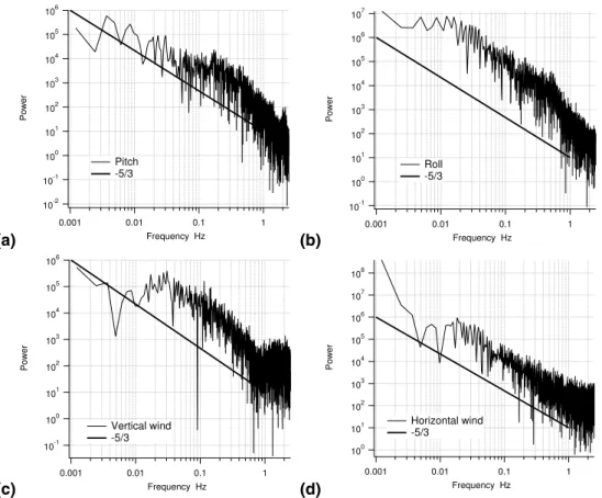
For this flight, only 5 Hz data were available so power spectral density (PSD)

informa-5

tion is only available up to 2.5 Hz. The ideal form for the PSDs is a uniform slope in the inertial sub-range of gradient –5/3 on a log-log plot, indicating that the probe is sampling all relevant frequencies correctly. Figure 6 shows the PSDs for pitch, roll, vertical wind speed and horizontal wind speed. Whilst not completely uniform in slope, the PSDs for pitch and roll and horizontal wind speed do not deviate significantly from

10

the ideal case. However, for the vertical wind component there is a significant devia-tion between 0.6–1.0 Hz. The reason for this is not understood at present, and would require data at higher frequencies to allow a more complete analysis.

6 Assessment and errors

Comparison with the AT4 during tight aerial manoeuvres, and with ground-based

in-15

struments during CSIP Flight 8 show the AIMMS to be working satisfactorily. Of par-ticular significance, the ability to map a wind field accurately is demonstrated. Given the good agreement with other instruments, the figure of±0.5 ms−1for the accuracy of

the horizontal wind speed given by Aventech is realistic. Power spectral densities con-forming well to the ideal also give confidence in the horizontal wind speed data. Since

20

the wind direction is computed from the two horizontal wind components, the accuracy of the wind direction will clearly be a function of the magnitude of those components, although at low wind speed this parameter is naturally highly variable.

Accuracy for position is not in doubt: both the AIMMS and the AT4 use the differential method for calculating position which is accurate to within 0.01 m. Similarly, data for

(17)

ACPD

7, 3519–3555, 2007

Title Page

Tables Figures

◭ ◮

Back Close

Full Screen / Esc

roll and heading agree extremely well between the two GPS systems. Data for pitch do not agree as closely, however it is thought the data from the AT4 su_ffers from variable lag compared to the AIMMS due to the manner in which it is calculated.

No estimate is made for errors in data computed in turns – for the purposes of this paper, the AIMMS was not calibrated to give reliable data under such conditions. There

5

was also no means of determining the absolute accuracy of the vertical wind speed, since there was no comparable independent dataset, although the power spectra sug-gest that some of the variance in the vertical wind speed is being lost.

7 Case studies: Flights 6 and 7 during IOP16

7.1 Synoptic situation

10

In contrast to the case study of Flight 8 discussed in Sect. 5.5, wind conditions indicated by the AIMMS during Flights 6 and 7 showed considerable variation across the CSIP area, indicating a convergence zone in the centre of the Northern box. The CSIP area was covered by a weak, mostly southerly flow ahead of cold-frontal cloud belt advancing slowly from the west. This resulted in a warm sunny day over much of

15

the region, with only shallow convection to start with. The first cumulus, at around 1000UTC were closely associated with topography in SE England and the Midlands. These soon developed over the whole area, but were restricted to a height of 3 km by a strong lid. By late afternoon the lid had weakened, and by 16:00 UTC cloud top had reached 6 km.

20

It is the presence of the convergence zone which makes this a critical test of the AIMMS, in that it requires the probe to be able to determine subtle variations in the wind field as well as more significant changes, often along a single flight leg. The ability to successfully map such a wind field would confirm the viability of this probe for atmospheric research.

25

(18)

ACPD

7, 3519–3555, 2007

Title Page

Tables Figures

◭ ◮

Back Close

Full Screen / Esc

7.2 Flight 6, IOP16, 18 August, 12:18–13:08

The wind speed and direction from the AIMMS as a function of position is shown in Fig. 7, which also shows data from the AWS mesonet and the UFAM wind profiler, with the Cessna flying the northern box route. As before, the AWS and profiler data are time-matched for the closest approach by the Cessna. Comparison with the wind

5

profiler is discussed in Sect. 7.4.

The wind speed was light and variable along the northern legs, becoming more

steady further south at 5–6 ms−1_{. The most remarkable feature of this flight is the}

dramatic change in wind direction from SW in the west to SE in the east which results in an apparent convergence on the centre of the northern box. As with the data for

10

Flight 8, the AWS mesonet agrees well with the AIMMS in terms of the broad pattern of wind circulation, although the AWS data appears to show that the convergence occurs more towards the southern edge of the box. Whilst it must be remembered that the AWS is representative of conditions at the surface, it is extremely encouraging in terms of assessing the quality of the AIMMS data that the AWS mesonet confirms the

15

existence of a convergence zone.

As expected, there were no significant trends in vertical wind speed, although there were some larger updrafts towards the eastern end of the southern leg of the box, where the standard deviation in the vertical wind speed was also high. Vertical wind speed was also highly variable on the eastern leg, although the average value was

20

close to zero.

Power spectral densities computed for this flight were found to be very similar to those shown for Flight 8 (see Fig. 6). Given the nature of the converging wind field, PSDs were calculated for all legs, but were found to be consistent. In general, levels of turbulence, indicated by the variances of the horizontal and vertical wind components,

25

(19)

ACPD

7, 3519–3555, 2007

Title Page

Tables Figures

◭ ◮

Back Close

Full Screen / Esc

of comparison as a function of position on the flight track.

7.3 Flight 7, IOP16, 18 August, 14:09–15:51

This flight took place on the same day as Flight 6, but occurred further on into the convective development phase. In general the wind field was similar to Flight 6, but with slightly higher wind speeds. The northern box was flown twice, with consistent

5

patterns in the wind field on the two passes.

Figure 9 shows wind speed and direction from the AIMMS as function of position for Flight 7, along with time-matched AWS and profiler data. Horizontal wind speed reached 7–8 ms−1 _{in the west, but dropped o}_ff_{almost to zero in the NE corner of the}

box. Once again, the marked feature of this flight was the dramatic change in wind

10

direction across the box, from westerly in the west to easterly in the east, and again an apparent convergence towards the centre of the northern box. The area with the lowest wind speeds appeared to have moved eastwards along the northern edge of the box by approximately 30 km over 21_/₂_{h between Flight 6 and the second pass of Flight}

7. Once again, the broad pattern of circulation is confirmed by the ground-based AWS

15

mesonet data and also by the point measurement provided by the wind profiler. Vertical wind speed remained highly variable on the eastern leg of the box for both passes (Fig. 8). In general standard deviations ofw,u,T and RH were relatively high for much of the northern and eastern legs of the flight. Combined with the variability in the wind direction in these areas, for both this and Flight 6, this strongly suggests

20

that a broad-scale meteorological feature was moving from west to east across the upper part of the box during the course of Flights 6 and 7. This feature is likely to have been a convergence line or zone, particularly given the striking pattern of wind direction observed by the AIMMS.

(20)

ACPD

7, 3519–3555, 2007

Title Page

Tables Figures

◭ ◮

Back Close

Full Screen / Esc

7.4 Comparison with the wind profiler for Flights 6, 7 and 8

The UFAM wind profiler operated by the University of Manchester was the only ground-based instrument to measure the wind vector close to the flight path of the Cessna during these flights. The profiler is a three antenna Doppler radar (UHF PCL1300) manufactured by Degreave Horizon. It is designed to measure the three components

5

of the wind vector twenty four hours a day to an accuracy of less than 1 ms−1for speed

and less than 10◦ _{for direction. The frequency of operation was 1290 MHz (L-band)}

with a peak power of 3.5 kW and a beam width of 8◦_{. The vertical range was between}

approximately 70 m and 3940 m with a resolution of 72 m. It must, however, be remem-bered that the profiler did not lie exactly on the flight path at any point, and that any

10

comparison with the AIMMS data is therefore complicated by this lateral displacement. A full description of the profiler is given by Norton et al. (2006).

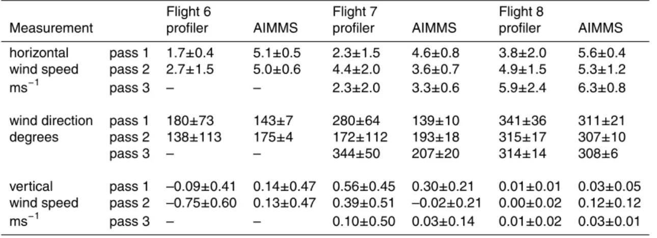
Table 4 shows a comparison of wind direction and horizontal and vertical wind speed from the AIMMS and the wind profiler, with the errors reflecting the spread of 1-min averaged values used to calculate the figures. Data is only shown for those legs of

15

the flights which pass closest to the profiler. Qualitative comparison between the two datasets is generally good for horizontal wind speed. Agreement is not quite so good for wind direction, although for both speed and direction agreement is quantitatively very good for Flight 8. This reflects the general stability of conditions experienced across the whole of the CSIP area for Flight 8. For Flights 6 and 7 the wind profiler

20

in particular shows how variable conditions were on even a short timescale, with wind direction changing markedly with height as well as time. The effect of this variability

is exacerbated by the lateral separation of the measurements, making it di_fficult to

compare vertical wind speeds, although di_fferences between the two instruments are

not significant.

(21)

ACPD

7, 3519–3555, 2007

Title Page

Tables Figures

◭ ◮

Back Close

Full Screen / Esc

8 Conclusions

A low-cost turbulence probe has been installed and used on the UFAM Cessna 182J, with encouraging results. The data has shown good comparison with other measure-ment methods, including ground-based observations and ground-based remote sens-ing. In particular, the probe has proved to be capable of reliably mapping out a

hori-5

zontal wind field over a large area.

The full capabilities of the probe in respect of assessing the absolute frequency re-sponse have not been tested for technical reasons, but all the available data shows the probe to be functioning in a manner consistent with being used for scientific research. Whilst the frequency response for horizontal wind speed and attitude is good, further

10

investigation is required with higher frequency data to test the full response of the probe for vertical wind speed.

Good quality data from this probe is entirely reliant on successful calibrations, but the procedures for these ensure the probe is easily installed and operated on most types of aircraft. The recent addition of a second CPM to the system has made the AIMMS

15

more useful as an on-line tool, as well as still being able to record full high frequency data: this is a significant deficiency in the standard system.

Further work will be carried out with 20 Hz data from the AIMMS. It is anticipated, from the data presented above, that the probe will in future be used to measure fluxes of atmospheric constituents such as trace gases and particulates.

20

Acknowledgements. The authors acknowledge funding from the UK NERC, and thank A. Blyth and K. Browning for their efforts in coordinating CSIP. We thank I. Stromberg for compiling and submitting the relevant paperwork to the UK CAA and EASA, B. Woodcock and S. Foster at Aventech for their support in setting up AIMMS, and B. Brooks at the University of Leeds for running the AWS network. At the University of Manchester we would like to thank M. Gray

25

for acting as reserve pilot for CSIP, M. Flynn for his work on the Cessna logging system and P. Kelly for fabrication of parts to enable the AIMMS to be certified.

(22)

ACPD

7, 3519–3555, 2007

Title Page

Tables Figures

◭ ◮

Back Close

Full Screen / Esc

References

Bange, J., Beyrich, F., and Engelbart, D. A. M.: Airborne measurements of turbulent fluxes during LITFASS-98: Comparison with ground measurements and remote sensing in a case study, Theor. Appl. Climatol., 73, 35–51, 2002

Bower, K. N., Beswick, K. M., Burgess, R. A., Stromberg, I. M., and Gallagher, M. W.: Aerosol

5

and Trace Gas Measurements over the Birmingham Conurbation during PUMA, Nucleation and Atmospheric Aerosols 2000: 15th Int. 7 Conf., edited by: Hale, B. N. and Kulmala, M., 2000

Brown, E. N., Friehe, C. A., and Lenschow, D. H.: The use of pressure fluctuations on the nose of an aircraft for measuring air motion, J. Climate Appl. Meteorol., 22, 171–180, 1983

10

Browning, K., Blyth, A., Clark, P., Corsmeier, U., Morcrette, C., Agnew, J., Bamber, D., Barthlott, C., Bennett, L., Beswick, K., Bitter, M., Bozier, K., Brooks, B., Collier, C., Cook, C., Davies, F., Deny, B., Engelhardt, M., Feuerle, T., Forbes, R., Gaffard, C., Gray, M., Hankers, R., T Hewison, Huckle, R., Kalthoff, N., Khodayar, S., Kohler, M., Kraut, S., Kunz, M., Ladd, D., Lenfant, J., Marsham, J., McGregor, J., Nicol, J., Norton, E., Parker, D., Perry, F., Ramatschi,

15

M., Ricketts, H., Roberts, N., Russell, A., Schulz, H., Slack, E., Vaughan, G., Waight, J., Watson, R., Webb, A., Wieser, A., and Zink, K.: The Convective Storm Initiation Project, Bulletin of the AMS, in press, 2007

DePriest, D.: NMEA Data,http://www.gpsinformation.org/dale/nmea.htm.

Gallagher, M. W., Choularton, T. W., Bower, K. N., Stromberg, I. M., Beswick, K. M., Fowler,

20

D., and Hargreaves, K. J.: Measurements of methane fluxes on the landscape scale from a wetland area in North Scotland, Atmos. Environ., 28(15), 2421–2430, 1994.

Gallagher M. W., Downer, R. M., Choularton, T. W., Gay, M. J., Stromberg, I. M., Mill, C. S., Radojevic, M., Tyler, B. J., Bandy, B. J., Penkett, S. A., Davies, T. J., Dollard, G. J., and Jones, B. M. R.: Case studies of of the oxidation of sulphur dioxide in a hill cap cloud using

25

ground and aircraft based measurements, J Geophys. Res., 95(D11), 18 517–18 537, 1990. Goddard, J. W. F., Eastment, J. D., and Thurai, M.: The Chilbolton Advanced Meteorological

Radar – A tool for multi-disciplinary atmospheric research, Electronics Communication Eng. J., 6(2), 77–86, 1994.

Hacker, J. M. and Crawford, T.: The Bat-Probe: The ultimate tool to measure turbulence from

30

any kind of aircraft (or sailplane), J. Technical Soaring, 13(2), 43–46, 1999.

(23)

ACPD

7, 3519–3555, 2007

Title Page

Tables Figures

◭ ◮

Back Close

Full Screen / Esc

D. J., Noguer, M., van der Linden, P. J., Dai, X., Maskell, K., and Johnson, C. A., Cambridge University Press, Cambridge, 881 pp, 2001

Johnson, H. D., Lenschow, D. H., and Danninger, K.: A new fixed vane for air motion sensing, Proceedings of the Fourth Symposium on Meteorological Observations and Instrumentation, 487–491, Denver, Colorado, April 1978.

5

Kalman, R. E.: A new approach to linear filtering and prediction problems, Transaction of the ASME-Journal of Basic Engineering, 35–45, March 1960.

Lenschow, D. H.: Vanes for sensing incidence angles of the air from an aircraft, J. Appl. Mete-orol., 10, 1339–1343, 1971.

Leslie, D. C.: Developments in the Theory of Turbulence, (First paperback edition 1983), Oxford

10

University Press, printed by Edward Bros Inc, Michigan, 1973.

McBean, G.: Climate change and extreme weather: a basis for action, Natural Hazards, 31, 177–190, 2004.

Naud, C. M., Muller, J. P., Slack, E. C., Wrench, C. L., and Clothiaux, E. E.: Assessment of the performance of the Chilbolton 3-GHz advanced meteorological radar for cloud-top-height

15

retrieval, J. Appl. Meteorol., 44(6), 876–887, 2005.

Norton, E. G., Vaughan, G., Methven, J., Coe, H., Brooks, B., Gallagher, M. W., and Longley, O.: Boundary layer structure and decoupling from synoptic scale flow during NAMBLEX, Atmos. Chem. Phys., 6, 433–445, 2006,

http://www.atmos-chem-phys.net/6/433/2006/.

20

Notess, C. B.: Flight-test investigation of turbulence spectra at low altitude using a direct method for measuring gust velocities, Wright Air Development Technical Report, 54–309, 1954. Senior, C. A., Jones, R. G., Lowe, J. A., Durman, C. F., and Hudson, D.: Predictions of extreme

precipitation and sea-level rise under climate – Mathematical Physical and Engineering Sci-ences, 360(1796), 1301–1311, 2002.

25

Smith, M. H., Consterdine, I. E., and Park, P. M.: Atmospheric loadings of maritime aerosol during a Hebridean cyclone, Q. J. Royal Meteorol. Soc., 115, 383–395, 1989.

Stromberg, I. M., Mill, C. S., Choularton, T. W., and Gallagher, M. W.: A case study of stably stratified airflow over the Pennines using an instrumented glider, Boundary-Layer Meteorol., 46, 153–168, 1989.

30

Telford, J. W. and Warner, J.: On the measurement from an aircraft of buoyancy and vertical air velocity in cloud, J Atmos Sci, 19(5), 415–423, 1962.

Whiteway, J. A., Pavelin, E. G., Busen, R., Hacker, J., and Vosper, S.: Airborne

(24)

ACPD

7, 3519–3555, 2007

Title Page

Tables Figures

◭ ◮

Back Close

Full Screen / Esc

ments of gravity wave breaking at the tropopause, Geophys. Res. Lett., 30(20), 2070, doi:10.1029/2003GL018207, 2003.

Webb, A. R., Kylling, A., Wendisch, M., and J ¨akel, E.: Airborne measurements of ground and cloud spectral albedos under low aerosol loads, J. Geophys. Res., 109D, D20205, doi:10.1029/2004JD004768, 2004.

5

Welch, G. and Bishop, G.: An introduction to the Kalmann Filter, In University of North Carolina at Chapel Hill, Department of Computer Science. Tech. Rep. 95-041, available at http://

russell-davidson.arts.mcgill.ca/e761/kalman-intro.pdf, 2004.

Wood, R.: PhD Thesis, University of Manchester Institute of Science and Technology, 1997. Wood, R., Stromberg, I. M., Jonas, P. R., and Mill, C. S.: Analysis of an air motion system on a

10

light aircraft for boundary layer research, J. Atmos. Oceanic Tech., 14(4), 960–968, 1997. Wood, R., Stromberg, I. M., and Jonas, P. R.: Aircraft observations of sea-breeze frontal

(25)

ACPD

7, 3519–3555, 2007

Title Page

Tables Figures

◭ ◮

Back Close

Full Screen / Esc

Table 1.Cessna flights during the main CSIP campaign in 2005.

Date Time Flight# IOP Flight Plan and way-points

29 June 10:43–11:40 1 5 East-West, 1 circuit, ABB’JKJA 4 July 10:48–11:35 2 6 East-West, 1 circuit, AJKI’A

13 July 10:23–13:12 3 8 East-West, partial Northern Box, 2 circuits, ABB’CIAJKABB’CIAJKI’A 13 July 14:38–16:23 4 8 East-West, partial Northern Box, 1 circuit, AJCIAJKAJCIA

11 August 15:46–16:57 5 14R Southern Box, 1 circuit, ABLMNOPBA 18 August 12:18–13:08 6 16 Northern Box, 1 circuit, AB’CDEFI’A

18 August 14:10–15:51 7 16 Northern Box, 2 circuits, AB’CDEFJCDEFB’A 19 August 14:11–16:14 8 17 Northern Box, 2 circuits, ABJCDEFGHDEFJA 25 August 08:05–10:11 9 18 Northern Box, 1 circuit, ABB’CDEFGHIA 25 August 13:24–14:44 10 18 North-South, 3 repeats, ABIBIBIA

(26)

ACPD

7, 3519–3555, 2007

Title Page

Tables Figures

◭ ◮

Back Close

Full Screen / Esc

Table 2.AIMMS specifications.

Module Specification

All modules power: 12.5-37VDC, 800-900mA at 12.5V

digital serial communication via 115kbaud controller area network Measurement frequency up to 20Hz

ADP Overall weight 3.36 kg Operating range –20◦_{C to}

+50◦_C

Static pressure range 0–110 kPa, accuracy 0.1 kPa±0.05%

Pitot pressure range 0–14 kPa, accuracy 0.02 kPa±0.05%

Wind speed horizontal: accuracy 0.5 ms−1 vertical: accuracy 0.75 ms−1 Temperature glass encapsulated bead thermistor

calibrated accuracy 0.05◦_{C (0.3}◦_{C with}

dynamic heating correction)

resolution 0.01◦_{C, time constant}_<_{5 s}

mounted in ventilated reverse-flow chamber Relative Humidity thermoset polymer capacitative

accuracy±2% RH (0–100%)

resolution 0.1%, time constant<5 s at 20◦_C

mounted in ventilated reverse-flow chamber Compass heading 3-axis magnetic field sensors

Communication external RS232 at 115kbaud IMU Overall weight 0.74 kg

Accelerometer 3-axis, range±5 g, accuracy 0.005 g, operated at 40 Hz

Rate gyro 3-axis, operated at 40 Hz GPS Overall weight 0.80 kg

Heading accuracy 0.1◦

Position accuracy 0.01 m

Antennae shares two dual frequency antennae with AT4 DGPS

CPM Overall weight 0.60 kg

Processor Motorola DSP56F807 processor 16Mbit flash memory

(27)

ACPD

7, 3519–3555, 2007

Title Page

Tables Figures

◭ ◮

Back Close

Full Screen / Esc

Table 3.Comparison between AIMMS and Javad AT4 attitude and position data.

Regression Regression

Measurement Slope (_±std. err) Intercept (_±std. err) R2

Latitude 0.999 (_±0.000) +0.030 (_±0.002) 1.00 Longitude 1.000 (_±0.001) +0.000(_±0.0003) 1.00 Heading 1.000 (_±0.000) +0.300(_±0.006) 0.99 Pitch 0.874 (_±0.004) –3.078 (_±0.003) 0.62 Roll 0.999 (±0.001) +1.912(±0.003) 0.99

(28)

ACPD

7, 3519–3555, 2007

Title Page

Tables Figures

◭ ◮

Back Close

Full Screen / Esc

Table 4.Comparison between the radar wind profiler and the AIMMS.

Flight 6 Flight 7 Flight 8

Measurement profiler AIMMS profiler AIMMS profiler AIMMS

horizontal pass 1 1.7±0.4 5.1±0.5 2.3±1.5 4.6±0.8 3.8±2.0 5.6±0.4

wind speed pass 2 2.7±1.5 5.0±0.6 4.4±2.0 3.6±0.7 4.9±1.5 5.3±1.2

ms−1 _{pass 3} _– _– _2.3

±2.0 3.3±0.6 5.9±2.4 6.3±0.8

wind direction pass 1 180±73 143±7 280±64 139±10 341±36 311±21

degrees pass 2 138±113 175±4 172±112 193±18 315±17 307±10

pass 3 – – 344±50 207±20 314±14 308±6

vertical pass 1 –0.09±0.41 0.14±0.47 0.56±0.45 0.30±0.21 0.01±0.01 0.03±0.05

wind speed pass 2 –0.75±0.60 0.13±0.47 0.39±0.51 –0.02±0.21 0.00±0.02 0.12±0.12

ms−1 _{pass 3} _– _– _0.10

(29)

ACPD

7, 3519–3555, 2007

Title Page

Tables Figures

◭ ◮

Back Close

Full Screen / Esc

51.8

51.6

51.4

51.2

51.0

50.8

50.6

Latitude

-2.5 -2.0 -1.5 -1.0

Longitude Thruxton

B-Chilbolton B'-Kingsclere

G-Pangbourne H-Didcot C/H'-Grove

I-Swindon D-Blakehill

E-Yate

F-Trowbridge O-Bath

K-Clutton Hill

N-Franklyns Field

M-Tarrant Rushton L-Verwood

P-Bowerchalke

J-Greenham Common I'-Crossover

G'-Crossover

A-Andover

Northern Box Southern Box Eeast/West Transect 600

500 400 300 200 100 0

Terrain Altitude - metres above mean sea level

Fig. 1. Flight paths and way-points for the Cessna, showing the pre-determined northern box,

southern box and east/west transects.

(30)

ACPD

7, 3519–3555, 2007

Title Page

Tables Figures

◭ ◮

Back Close

Full Screen / Esc

East x North

y

x-y plane

turbulence probe

Airflow vector

Vertical z

Fig. 2. The relationship between the Earth and aircraft coordinates. Earth coordinates are

North, East and vertical, or xyz. Aircraft coordinates are longitudinal axis, lateral axis and vertical axis, orx′_y′_z′_.

Ψ =heading inxyz;θ=pitch inxyz;φ=roll inxyz;α=angle of attack inx′_y′_z′_;_β

(31)

ACPD

7, 3519–3555, 2007

Title Page

Tables Figures

◭ ◮

Back Close

Full Screen / Esc

RS232 CAN 28V

RS232 CAN CAN RS232 CAN CAN RS232 CAN CAN RS232 CAN 28V AIMMS GPS Module

AIMMS Inertial Module

AIMMS Central Processing Module Antenna

Antenna

Javad AT4 Antenna

Antenna Antenna

Antenna 12V Signal

Splitters

AIMMS Central Processing Module

RS232

Not used COM2PC#1

PC#2 COM1 COM2PC#2 Tail

Cabin Port Wing Starboard

Wing

PC#1 COM1 AIMMS

Probe

Fig. 3. Schematic of the Javad AT4 differential GPS and AIMMS modules. The figure shows

the optional second CPM unit which allows on-line data to be displayed whilst the first CPM records high frequency data.

(32)

ACPD

7, 3519–3555, 2007

Title Page

Tables Figures

◭ ◮

Back Close

Full Screen / Esc

Interactive Discussion Yaw 5-10 degrees to

port, then to starboard, wings level Lowest speed,

close to stall Lowest speed,

close to stall Highest

cruise speed Highest

cruise speed

Increase speed gradually over 2 minutes

Decrease speed gradually over 2 minutes

Climb or descend 2000 feet as

quickly as possible at constant airspeed

True north

45 turn

15 turn

15 turn 30

turn 30 turn

30 seconds per leg

Fig. 4. Schematic diagram of the two airborne calibration procedures for the AIMMS sensor:

(33)

ACPD

7, 3519–3555, 2007

Title Page

Tables Figures

◭ ◮

Back Close

Full Screen / Esc

51.6

51.4

51.2

51.0

-2.4 -2.2 -2.0 -1.8 -1.6 -1.4 -1.2 -1.0

Waypoint Profiler AWS x2

600

500

400

300

200

100

0

Altitude m

Wind Profiler

Scale: 5 ms-1

Fig. 5. Horizontal wind vector for Flight 8, including data from the wind profiler and the AWS

mesonet. For clarity, only the first pass round the northern box is shown, and the AWS data is scaled by a factor of 2.

(34)

ACPD

7, 3519–3555, 2007

Title Page Abstract Introduction Conclusions References Tables Figures ◭ ◮ ◭ ◮ Back Close

Full Screen / Esc

Printer-friendly Version Interactive Discussion (a) 10-2 10-1 100 101 102 103 104 105 106 Power

0.001 0.01 0.1 1 Frequency Hz

Pitch -5/3 (b) 10-1 100 101 102 103 104 105 106 107 Power

0.001 0.01 0.1 1 Frequency Hz

Roll -5/3 (c) 10-1 100 101 102 103 104 105 106 Power

0.001 0.01 0.1 1 Frequency Hz

Vertical wind -5/3 (d) 100 101 102 103 104 105 106 107 108 Power

0.001 0.01 0.1 1 Frequency Hz

Horizontal wind -5/3

Fig. 6. Power spectral densities for AIMMS data from Flight 8 for(a)pitch,(b)roll,(c)vertical

(35)

ACPD

7, 3519–3555, 2007

Title Page

Tables Figures

◭ ◮

Back Close

Full Screen / Esc

51.6

51.4

51.2

51.0

-2.4 -2.2 -2.0 -1.8 -1.6 -1.4 -1.2 -1.0

Waypoint Wind Profiler AWS x2

600

500

400

300

200

100

0

Altitude m

Wind Profiler

Scale: 5 ms-1

mesonet. The AWS data is scaled by a factor of 2.

(36)

ACPD

7, 3519–3555, 2007

Title Page

Tables Figures

◭ ◮

Back Close

Full Screen / Esc

✁✂

✄

☎

✆

✝

✞

Fig. 8. Summary of standard deviations and means for Flights 6 and 7, to show relative

varia-tions as a function of flight path.σ_w,σ_{f f} and u are in ms−1

,σ_T is given in◦_C,_σ

RHis given in %,

and TKE is given in m2s−2

(37)

ACPD

7, 3519–3555, 2007

Title Page

Tables Figures

◭ ◮

Back Close

Full Screen / Esc

51.6

51.4

51.2

51.0

-2.4 -2.2 -2.0 -1.8 -1.6 -1.4 -1.2 -1.0

Waypoint Profiler AWS x2

600

500

400

300

200

100

0

Altitude m

Wind Profiler

Scale: 5 ms-1

mesonet. For clarity, only the first pass round the northern box is shown, and the AWS data is scaled by a factor of 2.