Nat. Hazards Earth Syst. Sci., 13, 2805–2813, 2013 www.nat-hazards-earth-syst-sci.net/13/2805/2013/ doi:10.5194/nhess-13-2805-2013
© Author(s) 2013. CC Attribution 3.0 License.
Natural Hazards
and Earth System
Sciences
Wind-wave amplification mechanisms: possible models for steep
wave events in finite depth
P. Montalvo1,2, R. Kraenkel3, M. A. Manna1,2, and C. Kharif4,5
1Université Montpellier 2, Laboratoire Charles Coulomb, UMR5221, 34095, Montpellier, France 2CNRS, Laboratoire Charles Coulomb, UMR5221, 34095, Montpellier, France
3Instituto de Física Téorica, UNESP – Universidade Estadual Paulista, Rua Dr. Bento Teobaldo Ferraz 27, Bloco II, 01140-070, São Paulo, Brazil
4Ecole Centrale Marseille, 38 rue Frédéric Joliot-Curie, 13451 Marseille cedex 20, France
5Institut de Recherche sur les Phénomènes Hors Équilibre, CNRS, AMU, UMR7342, 49 rue Frédéric Joliot-Curie, BP 146, 13384 Marseille cedex 13, France
Correspondence to:M. A. Manna ([email protected])
Received: 10 June 2013 – Published in Nat. Hazards Earth Syst. Sci. Discuss.: 8 July 2013 Revised: 1 October 2013 – Accepted: 10 October 2013 – Published: 8 November 2013
Abstract. We extend the Miles mechanism of wind-wave
generation to finite depth. Aβ-Miles linear growth rate
de-pending on the depth and wind velocity is derived and al-lows the study of linear growth rates of surface waves from weak to moderate winds in finite depthh. The evolution of β is plotted, for several values of the dispersion parameter khwithkthe wave number. For constant depths we find that
no matter what the values of wind velocities are, at small enough wave age theβ-Miles linear growth rates are in the
known deep-water limit. However winds of moderate inten-sities prevent the waves from growing beyond a critical wave age, which is also constrained by the water depth and is less than the wave age limit of deep water. Depending on wave age and wind velocity, the Jeffreys and Miles mecha-nisms are compared to determine which of them dominates. A wind-forced nonlinear Schrödinger equation is derived and the Akhmediev, Peregrine and Kuznetsov–Ma breather solu-tions for weak wind inputs in finite depthhare obtained.
1 Introduction
The pioneer theories to describe surface wind-wave growth in deep water began with the works of Jeffreys (1925), Phillips (1957) and Miles (1957, 1997), and the modern in-vestigations take nonlinearity and turbulence effects into ac-count. Janssen (2004) has provided a thorough review of the topic.
1.1 Miles’ and Jeffreys’ mechanisms of wind-wave growth
Miles’ and Jeffreys’ theories consider both air and water to be incompressible and disregard viscosity effects. Both the-ories are linear and Miles’ mechanism is limited to the deep-water domain. They give the linear wave growthγMiles and γJeffreys (respectively noted γM and γJ) of wind-generated
normal Fourier modes of wave numberk. In Miles’ theory
the basic state is a shear current in air and still water. The air turbulence is disregarded (Janssen, 2004) aside from estab-lishing the logarithmic profile of the wind flow. The Miles mechanism of wave generation by wind states that waves are produced and amplified through a resonance phenomenon. Resonance appears between the wave-induced pressure gra-dient on the inviscid airflow and the surface waves. The reso-nant mechanism happens at a critical height where the airflow speed matches the phase velocity of the surface wave.
Jeffreys computedγJfor deep water (Jeffreys, 1925) and for
finite depth as well (Jeffreys, 1926). Airflow separation oc-curing only over steep waves (Banner and Melville, 1976; Kawai, 1982), the Jeffreys sheltering mechanism must be ap-plied locally in time and space rather than constantly and ev-erywhere on the wave field. Note that the sheltering mech-anism is working even without proper airflow separation. In fact, there is a thickening of the boundary layer (Reul et al., 2008) on the leeward side that generates a pressure asymme-try and consequently a sheltering effect.
1.2 The Miles and Jeffreys mechanisms in finite depth: basis to model freak wave events in coastal regions
Generally extreme wave events occur in the presence of wind. Kharif et al. (2008) and Touboul and Kharif (2006) investigated the influence of wind on extreme wave events using the Jeffreys sheltering theory. They have shown that extreme events may be sustained longer by the airflow sep-aration. This mechanism can only be invoked if the wave is steep enough to effectively separate the airflow. Otherwise, for a too-low steepness parameter ka the Jeffreys sheltering mechanism due to flow separation becomes irrelevant.
Miles’ and Jeffreys’ mechanism of wind-generated sur-face waves in deep water was used in Touboul et al. (2008) to describe (theoretically and numerically) the evolution of a chirped wave packet under wind forcing. A comparison of theγMand theγJvalues corresponding to a modified Jeffreys mechanism was developed.
However, all this work is limited to deep water and hence unable to fully describe winds generating nearshore waves where the wave field is influenced by bottom bathymetry. Consequently they are not adequate to correctly describe the wind influence on extreme wave events in the coastal zone.
Therefore an extension of Miles’ theory of wind-generated monochromatic waves to the case of finite depth under weak or moderate winds is needed, as well as a theoretical formu-lation of Jeffreys’ theory in terms of adequate finite depth parameters.
1.3 Nearshore extreme wave events
Extreme wave events are anomalous large-amplitude surface waves. They are calledfreakorrogue waves.It is crucial to understand the physical mechanisms producing freak waves, as well as to obtain an accurate prediction of their dynam-ics in extreme sea states. A number of mechanisms gener-ating freak waves have been identified. Such mechanisms are, for instance, linear space–time focusing, variable cur-rents, interaction waves/curcur-rents, modulational or Benjamin– Feir (BF) instability. A classical way to model the BF insta-bility is to use the nonlinear Schrödinger equation (NLS), as in references Touboul and Kharif (2006), Touboul et al. (2008), Kharif et al. (2008) and Onorato and Proment (2012).
However, in these papers, the NLS equation was used in deep water. In a recent paper Didenkulova, Nikolkina and Peli-novsky (2013) have described and compared properties of rogue waves in intermediate depth with those in deep water. The focused regime of the BF instability was studied using a NLS equation in arbitrary depth.
In this work we are able to produce an adequate model for nearshore extreme wave events.This is done using our finite depth extensions of Miles’ theory and the NLS equation in finite depth under the wind action. The case of a Jeffreys type wind input is straightforward.
NLS is exactly solvable, and some of its deterministic so-lutions are good candidates to be weakly nonlinear proto-types of rogue waves in finite depth under wind input. This is the case of the Akhmedian, Peregrine and Kusnetsov–Ma solutions.
The aims of this paper are: (i) to extend the Miles mech-anism to a finite depth setup, (ii) to express the Jeffreys mechanism in terms of adequate dimensionless parameters, (iii) to determine, in terms of wave age and wind velocity, which among the Miles and Jeffreys mechanisms prevails and (iv) to derive a wind-forced nonlinear Schrödinger equa-tion (NLS) in finite depth to study the effects of wind and depth on extreme wave events due to the modulational insta-bility.
The paper is organized as follows. In Sects. 2, 2.1 and 2.2 the linear stability problem of the air–water interface is pre-sented and the derivation of the system of equations coupling the waves to the airflow with the corresponding dispersion re-lation is done. In Sects. 3, 3.1 and 3.2, we write the growth rates of Miles’ and Jeffreys’ theories, with appropriate scal-ings and variables. In Sect. 4.1 the Miles coefficient β is
plotted as a function of wave age withkhconstant. Next in
Sect. 4.2, we present our results about the evolution of the growth rate as a function of the wave age with h constant
for several wind velocities. A comparison between Miles’ and Jeffreys’ theory is shown and discussed in Sect. 4.3. In Sect. 5 we derive a wind-forced NLS equation in finite depth
h. The Akhmediev, Peregrine and Kuznetsov–Ma breather
solutions for weak wind inputs in finite depthhare exhibited.
Finally in Sect. 6, conclusion and perspectives are drawn.
2 Coupling of the air and water dynamics at the interface
The fluid particle coordinates are expressed in a fixed 3-dimensional Cartesian frameOxyz,Ozbeing the upwards
axis. We assume the problem to be invariant on they axis,
reducing the problem to an area parallel toOxz. We define
the surfacez=0 as the rest state of the interface. The
inter-face perturbation itself is denoted byηand depends on(x, t ).
The water depth is set at−h, and the air extends from the
2.1 Water dynamics
The horizontal and vertical components of the fluid velocity areuandw, both depending on(x, z, t ). They obey the linear
Euler equations of motion in finite depth (Lighthill, 1978):
ux+wz=0, ρwut = −Px, ρwwt = −Pz, (1)
w(−h)=0 at z= −h, (2)
ηt=w(0) at z=η(x, t ), (3)
P (η)=Pa(η)+ρwgη−P0 at z=η(x, t ). (4)
HereP =p+ρwgz−P0is a reduced pressure withpthe
pressure,P0 the total atmospheric pressure, g the
gravita-tional acceleration and ρw the water density.p and P
de-pend on(x, z, t )as well, and subscripts in u,w andP
de-note partial derivatives. We solve the linear equations system Eqs. (1)–(3) with
P =P(z)eiθ, u=U(z)eiθ,
w=W(z)eiθ, η=η0eiθ, (5)
whereP,U andWare to be found.We have the phaseθ= k(x−ct )withkthe wave number andcthe phase speed.η0 is an unknown constant. Using Eqs. (1)–(3) we obtainu,w
andP for all(x, z, t ). Then, using Eq. (4) we derive
ρwη0eiθ{c2kcothkh−g} +P0=Pa(η). (6)
In the Archimedean case,Pa(η)=P0and Eq. (6) returns the classical phase speed expression,
c2=c20=g
ktanh(kh). (7)
We need an expression forPaatz=ηto obtain the
modi-fiedc.
2.2 Air dynamics
We examine the steady state of a prescribed horizontal air-flow, with a mean velocityU depending only onz. We
de-note physical quantities in the air domain by a subscript a. The air density isρa; the perturbations to this steady state are
assumed to beua,wafor the velocities andpa for the non-reduced pressure, all quantities depending on(x, z, t ). Now,
using a reduced pressurePa=pa+ρagz−P0, we have
ua,x+wa,z=0, (8)
ρaua,t+U (z)ua,x+U′(z)wa
= −Pa,x, (9)
ρawa,t+U (z)wa,x
= −Pa,z, (10)
with primes indicating differentiation with respect toz. Next
we assume Pa=Pa(z)eiθ, ua=Ua(z)eiθ, wa=Wa(z)eiθ
and we add the boundary conditions onWaandPa,
lim
z→+∞(
Wa′+kWa)=0, (11)
lim
z→z0
Wa=W0, (12)
lim
z→+∞Pa=0, (13)
whereW0is a wind forcing at the surface level. It ensures
that there is always an interaction between the wind and the free surface. The pressure and the wind perturbations vanish at high altitudes. For the air, there is a kinematic condition as well at the aerodynamic sea surface roughness z0, over
the free surfaceη. In this work,z0will be determined by the Charnock relation (Charnock, 1955):
z0=αcu 2
∗
g, (14)
where u∗ is the friction velocity, and assuming that αc= 0.018 remains constant. The kinematic boundary condition
reads
ηt+U (z0)ηx=wa(z0). (15)
Our steady airflowU (z)is set as the logarithmic wind
pro-file
U (z)=U1ln(z/z0), U1=u∗
κ , κ≈0.41, (16)
whereκis the Von Kármán constant. Such a profile is a
com-mon ground to describe wind phenomena close to the marine boundary layer (Garratt et al., 1996). Hence, we can reduce Eq. (15) to
ηt=wa(z0). (17)
Then, using Eqs. (8)–(10) and (13) we obtain
wa=Waeiθ, (18)
ua= i
kWa,ze
iθ, (19)
Pa=ikρaeiθ
∞
Z
z
U (z′)−cW
a(z′)dz′. (20)
The Rayleigh equation (Rayleigh, 1880) is then found by eliminating Pa from Eqs. (9)–(10), and is valid as long as
z > z0
(U−c)(Wa′′−k2Wa)−U′′Wa=0. (21)
This equation contains a singularity at a so-called critical heightzc, whereU (zc)=c. All turbulence phenomena being
disregarded, any possible eddies are assumed to be set below
z0, and their influence is not taken into account. We note that Wa(z)andcare unknown in Eqs. (18)–(21). So, we have to
evaluatePa(η)to getc. We then have
pa(η)=P0−ρagη+ikρaeiθ
∞
Z
z0
[U (z)−c]Wa(z)dz, (22)
where z=z0 replaces z=η as the lower integral bound,
since we are studying the linear problem. Finally, eliminating the termikρaeiθ using Eq. (17), we derive
g(1−s)+csk
2
W0I1−c 2sk2
W0I2+kcoth(kh)
wheres=ρa/ρwandI1=R∞
z0 UWadz,I2=
R∞
z0 Wadz. As
the ratio densitys is of order of magnitude 10−3, we can
develop the wave speed in Eq. (23) asc=c0+sc1+o(s2).
Next, we findc1as a function ofWa, which is obtained by
solving Eq. (21) withc≈c0.
3 TheγMandγJwind inputs
3.1 γMwind input
The imaginary part of c gives directly the growth rate of η(x, t ):
γM=kℑ(c). (24)
All the physical quantities derived from the growth rate
γM can be expressed with three parameters: δ,θdwandθfd (Young, 1997a, b):
δ= gh
U12, θdw=
1
U1
r
g k,
θfd=θdwtanh1/2 δ θdw2
!
. (25)
The dimensionless parameterδ1/2, for constanth,
mea-sures the relative value of the shallow-water speed with re-spect toU1. The parameterθdw, equivalent of the wave age in
deep water, measures the phase speed relatively to the char-acteristic wind parameterU1in deep water, andθfd(a finite
depth wave age) measures the influence of the finite depth on
θdw.
In experiments, wether in wave tank or in field, the param-eterCpis used.Cp is the observed phase speed at the peak frequencyp. In this paper we used in Eq. (25) the phase
velocityc=ω/ kof one mode instead ofCporp. Next we
choose dimensionless variables (topped by hats)
U=U1U,ˆ Wa=W0Wˆa, z=zˆ k,
c=U1c,ˆ t=U1
g t.ˆ (26)
Using Eqs. (25) and (26) in Eq. (23) and discarding terms of order two inswe obtainc,
ˆ
c(δ, θdw)=θdwT1/21−s
2
+s2nTIˆ1−θdwT3/2Iˆ2
o
, (27)
whereT =tanh δ
θdw2 . Withe
γMt, we obtain the dimensionless
growth rateγˆM=U1 g γMas
ˆ γM= s
2
(
Tℑ(I1)
θdw2 −
T3/2ℑ(I2) θdw
)
. (28)
We have the following transformation rule betweenβ and
the dimensionlessγˆM(Montalvo et al., 2013):
β=2γˆM
s θ
3
dwT1/2. (29)
The dimensional mean energy growth rate,
ŴM= 1
hEi
∂E
∂t
, (30)
can then be written as a function ofβ:
ŴM=sβU12
k3
g
1/2
coth1/2(kh). (31)
3.2 γJwind input
Jeffreys (1926) established that the pressure component act-ing on a surface wave can be written as
Pa,Jeffreys=Pa,J=Sρa(U10−c)2ηx, (32)
whereηis the free surface elevation;S is the sheltering
co-efficient, always lower than unity; andU10 is the 10 m wind velocity. This is only valid when the wave slope is larger than a certain critical value. Such a pressure gradient can also be obtained when the boundary layer thickness varies from one side of the wave crest to another, thickening on the leeward slope and resulting in a non-separated sheltering (Belcher and Hunt, 1993). We do not consider variations of the bound-ary layer here. Then Jeffreys assumed that the rate of work transfer from the wind to the wave is (average with respect to time)
∂E
∂t
=
Pa,J·
−∂η ∂t
. (33)
Our study being perturbative, we do not have any informa-tion on the possible value ofηwhatsoever. We assume a
si-nusoidal wave of the formη=η0cosk(x−ct ),η0being the
wave amplitude. With this, and recalling that the mean wave energy is hEi =ρwgη
2 0
2, we can deduce the energy growth rate expression
ŴJ=k 2
gcsS(U10−c)
2. (34)
Now, in order to transformU10intoU1, the relevant wind
scale, we use the wind-stress coefficientC10, as defined by Wu (1982) and the Charnock relation (Charnock, 1955):
C10=(0.8+0.065U10)×10−3= u
2
∗
U102 , (35)
U1=U10
κ
p
C10. (36)
Fig. 1.The drag coefficient versus theU10 wind velocity. As we
can see, it follows a linear progression until its maximum around 30 m s−1, then decreases. So, a linear parametrization ofC
10 is a reasonable approximation.
conditions. However, above a 30 m s−1limit, the drag coef-ficient drops off theU10 linear progression in Eq. (35), as
we can see in Fig. 1. This phenomenon reported in Powell et al. (2003) is due to the droplet saturation in a suspension layer above the sea surface. Even though it is possible to use the model developed in Makin (2004) to calculate the correct drag coefficient and friction velocity, flow separation is likely to occur at wind speeds that high, preventing Miles’ mecha-nism from acting. Hence, we keep the range of wind speeds below this limit for computation and we can use Eqs. (35) and (36).
4 Results
In the following Sects. 4.1, 4.2, 4.3 and 5 we present (i) the evolution of the finite depth wind-wave inputβwithθdwfor
khconstant; (ii) its evolution, as a function of wind
veloc-ity and wave age, with h constant; (iii) a comparison
be-tween the Miles and Jeffreys mechanism for finite depth; and (iv) a wind-forced NLS equation in finite depth.
After recalling several approximations, we are going to work with the finite depthβ-Miles wind input instead ofγˆM. 4.1 The finite depthβ-Miles with constantkh
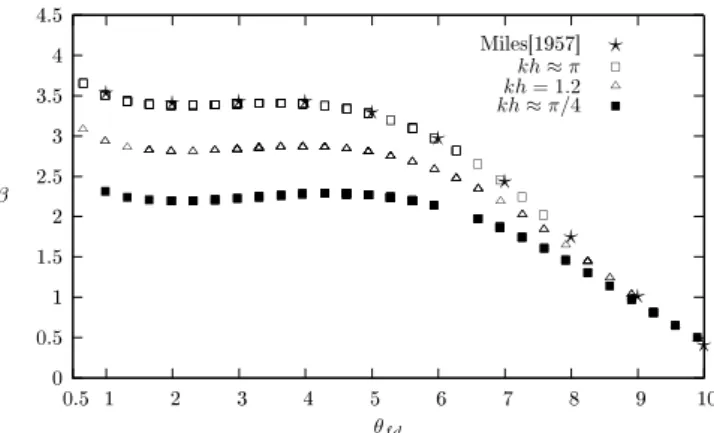
First, we plot in Fig. 2 the evolution of the growth rate with
θfdfor several constant values of thekhparameter. Neitherk
norhare constants,
– for large values of the theoretical wave ageθfd, the
val-ues ofβare in the deep-water limit,
– from small to intermediate values ofθfd the values of
βare lower than in the deep-water limit and
dβ
dθfd ∼0.
✵ ✵✳✺ ✶ ✶✳✺ ✷ ✷✳✺ ✸ ✸✳✺ ✹ ✹✳✺ ✵✳✺ ✶ ✷ ✸ ✹ ✺ ✻ ✼ ✽ ✾ ✶✵ β
θf d
▼✐❧❡s❬✶✾✺✼❪ ⋆ ⋆ ⋆ ⋆ ⋆ ⋆ ⋆ ⋆ ⋆ ⋆ ⋆
kh≈π
kh= 1.2
△ △ △ △ △ △ △△ △ △△ △ △ △ △ △ △ △ △△ △ △ △ △ △ △ △ △ △ △ △ △ △ △ △ △ △ △ △ △ △ △ △ △ △ △ △ △ △ △ △ △ △ △ △ △ △ △ △ △ △ △ △ △ △ △ △ △ △ △ △ △ △ △ △ △ △ △ △ △ △ △ △ △ △ △ △ △ △ △ △ △ △ △△ △△ △△△△△ △ △△ △△ △ △ △ △ △ △ △ △ △ △
kh≈π/4
Fig. 2.Miles’βvsθfd. For the deep-water limitkh≈π our results
fit the Miles curve.kh < π/4 corresponds to shallow water that is beyond the range of validity of our model. An intermediate value ofkhis included, and we see thatβis less than in the deep-water limit.
The small values of θfd seem constrained. In fact, be-cause all the curves are calculated with the same parame-ter spaceh∈ [0.1 m,18 m], different bounds onkhgive
dif-ferent bounds onk, and subsequently on θfd. For the
deep-water limitkh≈π we rediscover Miles’ result, and below
the shallow-water limitkh≈π/4 we are beyond the validity
of the model.
4.2 The finite depth β-Miles from weak to moderate winds withhconstant
In deep water, we have the classical Miles curve β(θdw).
Herein, the introduction of the parameter δ transforms the
unique curve of wave growth rate infamilies of curvesβ(θfd)
indexed byδ=gh/U12, i.e. a curve for each value ofδ. Two
types of families are possible:
– a family ofβcurves againstθfdindexed byhwithU1 constant;
– a family ofβ curves againstθfdindexed byU1, withh
constant.
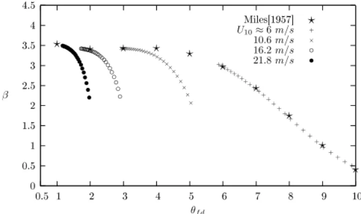
The first one was studied in Montalvo et al. (2013). In this work, and for the first time, we presented curves of wave growth evolution as a function ofU1with constant depthh.
Figures 3, 4 and 5 showβcurves for constanthas a function
ofθfd, for friction velocitiesU1from 0.5 to 2.5 m s−1. More
specifically, this denomination refers to a 10 m wind velocity, namelyU10, such that
5< U10<22 m s−1.
One can switch fromU1 to U10 using simply Eq. (36). From now on, we will refer to U10 only. The curves show
✵ ✵✳✺ ✶ ✶✳✺ ✷ ✷✳✺ ✸ ✸✳✺ ✹ ✹✳✺ ✵✳✺ ✶ ✷ ✸ ✹ ✺ ✻ ✼ ✽ ✾ ✶✵ β
θf d
▼✐❧❡s❬✶✾✺✼❪ ⋆ ⋆ ⋆ ⋆ ⋆ ⋆ ⋆ ⋆ ⋆ ⋆ ⋆ U10≈6m/s
+ + + + + + + + + + + + + + + + + + + + + + + + + + + +
10.6m/s
× × × × × × × × × × × × × × × × × × × × × × × × × × × × ×
16.2m/s
◦ ◦ ◦ ◦ ◦ ◦ ◦ ◦ ◦ ◦ ◦ ◦ ◦ ◦ ◦ ◦ ◦ ◦ ◦ ◦ ◦ ◦ ◦ ◦ ◦ ◦ ◦ ◦
21.8m/s
• • • • • • • • • • • • • • • • • • • • • • • • • • • •
Fig. 3.βvs.θfd, the wave-age-like parameter. The water depth is h=3 m for all curves above. For this depth, all 10 m wind speeds account for early drops in the growth rate. The deep-water limit
kh→ ∞, originally computed by Miles, is plotted for comparison. For the lower wind speed, the growth drop occurs closer to deep water. AlthoughU10=6 m s−1gives a deep-water-like behaviour, we see that stronger winds imply early (wavelength-wise) drops in the growth rate.
✵ ✵✳✺ ✶ ✶✳✺ ✷ ✷✳✺ ✸ ✸✳✺ ✹ ✹✳✺ ✵✳✺ ✶ ✷ ✸ ✹ ✺ ✻ ✼ ✽ ✾ ✶✵ β
θf d
▼✐❧❡s❬✶✾✺✼❪ ⋆ ⋆ ⋆ ⋆ ⋆ ⋆ ⋆ ⋆ ⋆ ⋆ ⋆ U10≈10.6m/s
× × × × × × × × × × × × × × × × × × × × × × × × × × × × ×
16.2m/s
◦ ◦ ◦ ◦ ◦ ◦ ◦ ◦ ◦ ◦ ◦ ◦ ◦ ◦ ◦ ◦ ◦ ◦ ◦ ◦ ◦ ◦ ◦ ◦ ◦ ◦
◦ 21.8m/s ◦
• • • • • • • • • • • • • • • • • • • • • • • • • • • •
Fig. 4.Same as Fig. 3 withh=9 m. The lowest wind speedU10≈
6.0 m s−1 is not shown, as the next one already gives us a
deep-water limit. ✵ ✵✳✺ ✶ ✶✳✺ ✷ ✷✳✺ ✸ ✸✳✺ ✹ ✹✳✺ ✵✳✺ ✶ ✷ ✸ ✹ ✺ ✻ ✼ ✽ ✾ ✶✵ β
θf d
▼✐❧❡s❬✶✾✺✼❪ ⋆ ⋆ ⋆ ⋆ ⋆ ⋆ ⋆ ⋆ ⋆ ⋆ ⋆ U10≈10.6m/s
× × × × × × × × × × × × × × × × × × ×
16.2m/s
◦ ◦ ◦ ◦ ◦ ◦ ◦ ◦ ◦ ◦ ◦ ◦ ◦ ◦ ◦ ◦ ◦ ◦ ◦ ◦ ◦ ◦ ◦ ◦ ◦ ◦
◦ 21.8m/s ◦
• • • • • • • • • • • • • • • • • • • • • • • • • • • •
Fig. 5.Same as Fig. 4 withh=18 m.
– no matter what the values of wind velocities are, at
small enough wave ageθfdthe growth rateβ satisfies
the known deep-water limit;
– the consequences of finite h are visible as θfd
aug-ments. The coefficient β is lesser than in the
deep-water limit. Furthermore, if the finite depth wave age
θfdis kept constant, the growth rateβ decreases as the
wind speedU10augments.
EachU10curve approaches its owntheoreticalθfd-limited growthasβgoes to zero (no energy transfer). Then, the wave
propagates steadily without changing its amplitude. Theθfd at which this happens is lower as the wind speed augments. Consequently, developed seas are reached faster under mod-erate winds than under weak winds. The evolution ofβunder
wind intensity and wave age shown in Figs. 3, 4, and 5 is not a dynamical one, but rather a collection of wave snapshots taken at every step of the growth in height and age.
4.3 ComparisonγMversusγJ
Very recently, Tian and Choi (2013) investigated experimen-tally and numerically the evolution of deep-water waves in-teracting with wind, with breaking effects. They discussed the relative importance of Miles’ and Jeffreys’ models and showed that Miles’ model may be used for waves of mod-erate wave steepness under weak to modmod-erate wind forc-ing, whereas for steep waves under strong wind forcing both mechanisms may have to be considered. In this section we desire to measure the relative importance of Miles’ mecha-nism versus Jeffreys’ mechamecha-nism in finite depth. To do that, we follow the idea in Touboul and Kharif (2006). Taking the derived growth rates from Sects. 3.1 and 3.2, one can establish the ratio between them. It reads, with only non-dimensional parameters,
R= ŴJ
ŴM =
tM
tJ =
ST
β
κ
√
C10 −θfd
, (37)
where tM=Ŵ−M1 and tJ=Ŵ−J1 are the characteristic
timescales of growth for the Miles and Jeffreys mechanism. Hence, we can calculateR(U10, θfd)to study the evolution of
this ratio with the theoretical wave age, for different values of the wind speed. Each point in the(θfd, U10)plane
corre-sponds to a water depthhbetween 3 m and 18 m and a
dis-persive parameterkh∈π4;π. These boundaries onkh
Fig. 6.(U10, θfd)parameter space for continuously varying values
ofR=ŴJ/ ŴM. In the domain defined byR <1, the Miles
mech-anism is dominant, whereas forR >1 the Jeffreys mechanism is
dominant.
5 Wind-forced nonlinear Schrödinger equation in finite depth
Let us consider the air/water system from a quasi-linear point of view; i.e. the water dynamics is considered nonlin-ear and irrotational and, as in Miles’ theory, the airflow is kept linear. So with this assumption the complete irrotational Euler equations and boundary conditions in terms of the ve-locity potentialφ (x, z, t )are
φxx+φzz=0 for −h≤z≤η(x, t ), (38)
φz=0 for z= −h, (39)
ηt+φxηx−φz=0 for z=η(x, t ), (40)
φt+
1 2φ
2
x+
1 2φ
2
z+gη= −
1
ρwPa for z=η(x, t ). (41) In Miless’ theory of wave generation (Miles, 1957, 1997), the complex air pressurePacan be separated into two
com-ponents, one in phase and one in quadrature with the free surfaceη. A phase shift between those two quantities is
nec-essary to transfer energy from the airflow to the wave field. The transfer is only due to the part ofPain quadrature with
η. Hence, we will deal only with the acting pressure
compo-nent, that is,
Pa(x, t )=ρaβU12ηx(x, t ), (42)
so that the modified Bernoulli equation reads
φt+
1 2φ2x+
1
2φz2+gη= −sβU12ηx for z=η(x, t ). (43)
From Eqs. (38), (39), (40), and (43) we find a wind-forced finite depth NLS equation forηas a function of the standard
slow space and time variables ξ=ε(x−cgt ) andν=ε2t,
withε≪1 andcg the group velocity. The perturbed NLS equation reads
iην+aηξ ξ+b|η|2η=idη, (44)
withcg,a,banddgiven by Eqs. (45), (46), (47), and (48):
cg=c
2[1+2kh/sinh(2kh)], (45)
a= −c
2
g−gh[1−khT (1−T2)]
2ω , (46)
b= k
4c2
4ωT2
9
T2−12+13T
2
−2T4−2[2c+cg(1−T
2)]2
gh−c2g
#
, (47)
d=sβ
2
U12
c2T ω. (48)
For more information about the derivation of the coeffi-cients a and b see Thomas et al. (2012). To derive a
di-mensionless wind-forced NLS equation we use Eq. (26) and we obtain in the original laboratory variablesx andt (after
a Galilean transformation in order to eliminate the linear term
cgηxand dropping the hats)
iηt+Aηxx+B|η|2η=iDη, (49)
withcg,A,B, andDnow given by Eqs. (50), (51), (52) and
(53):
cg= 1 2θfd
"
1+ δ θdw2
1−T2 T
#
, (50)
A= −
cg2−δh1−δθdw−2(1−T2)i
2θfdθdw2 , (51)
B= 1
4T2θfd3θdw2
9
T2−12+13T
2
−2T4−
2h2θfd−1+cg(1−T2)i2 δ−cg2
, (52)
D=sβ
2
T1/2
θdw3 . (53)
Equation (49) is a wind-forced finite depth NLS equation in dimensionless variables.
5.1 The Akhmediev, Peregrine and Ma solutions for weak wind inputs in finite depth
Didenkulova, Nikolkina and Pelinovsky (2013) studied the Peregrine breather in water of finite depth without the wind influence. The present work allows, for the first time, similar studies in finite depth with the right Miles growth rates.
In the following we are going only to consider the so-called focusing NLS equation, i.e. positivesAandB.
Intro-ducingη′andx′as η′=√Bη, x′=√x
A,
Eq (49) transforms, dropping the primes, into
iηt+ηxx+ |η|2η=iDη. (54)
Introducing a functionM(x, t )as
M(x, t )=η(x, t )exp(−Dt ), (55)
we obtain from Eq. (54)
iMt+Mxx+exp(2Dt )|M|2M=0. (56)
In order to reduce Eq. (54) into the standard form of the NLS with constant coefficients we proceed in the follow-ing way. First of all we consider the wind forcfollow-ing 2Dt to
be weak, such that the exponential can be approximated so we have
iMt+Mxx+n|M|2M=0, n=n(t )=
1
1−2Dt. (57)
Now with a change of coordinates from(x, t )to(z, τ )
de-fined by
z(x, t )=xn(t ), τ (t )=t n(t ), (58)
and scaling the wave envelope as (Onorato and Proment, 2012)
M(z, τ )=9(z, τ )pn(τ )exp
−iDz2 n(τ )
, (59)
we reduce Eq. (57) to the standard focusing equation for
9(z, τ ):
i9τ+9zz+ |9|29=0. (60)
Equation (60) admits well-known breather solutions that are simple analytical prototypes for rogue wave events. They are the Akhmediev (9A) (Akhmediev et al., 1987), the
Pere-grine (9P) (Peregrine, 1983) and the Kuznetsov–Ma (9M)
(Ma, 1979) breather solutions.
Dysthe and Trulsen (1999) investigated whether freak waves in deep water could be modelled by 9A, 9P or by
9M. Onorato and Proment (2012) considered the influence
of weak wind forcing and dissipation on these 9A,9P or
9Msolutions in deep water.
The present work allows us to go ahead and to exhibit ex-pressions for9A,9P and9M under the influence of weak wind forcing in finite depthh given by the extended Miles mechanism.These solutions read (Dysthe and Trulsen, 1999)
ηA=P (τ )
cosh(τ
−2iω)−cos(ω)cos(pz)
cosh(τ )−cos(ω)cos(pz)
, (61)
withp=2 sin(ω),=2 sin(2ω),ωreal andprelated to the
spatial period 2π/p,
ηP =P (τ )
1− 4(1+4iτ ) 1+4z2+16τ2
, (62)
ηM=P (τ )
cos(τ
−2iω)−cosh(ω)cosh(pz)
cosh(τ )−cos(ω)cos(pz)
, (63)
withp=2 sinh(ω),=2 sinh(2ω)andreal and related to
the time period 2π/ and
P (τ )=n(τ )exp
−iDz2 n(τ )
exp[2iτ].
A more detailed analytical and numerical analysis in terms ofxandtof Eq. (49) will be developed in a future work.
6 Conclusions
We have extended the well-known Miles theory to the finite depth case under breeze to moderate wind conditions. We have linearized the equations of motion governing the dy-namics of the air/water interface problem in finite depth, and we have investigated the linear instability in time of a nor-mal Fourier mode of wave numberkin Miles’ and Jeffreys’
mechanisms in finite depth. For the Miles mechanism we have shown that normal modes are unstable and grow ex-ponentially in time as
exp
"
sβ
2θfd3T1/2
#
t,
withβ the finite depth Miles coefficient. The curves of β
againstθfdwithkhconstant showed essentially that the
val-ues of β remain smaller than those corresponding to the
deep-water limit∀θfd. Wind effects on the temporal growth
have been discussed. From a comparison between the growth ratesγMandγJa diagram in the (θfd,U10) plane displays the
domains where the Miles mechanism (R <1) or the Jeffreys
mechanism (R >1) is dominant.
In this paper we have used the conventional finite depth NLS second-order envelope equation under the wind action. The third-order finite depth NLS equations introduced by Slunyaev (2005) could improve the results.
Other factors influence the mechanisms of wave growth under wind action, in finite depth: for instance, time varia-tions of wind speed and wind direction, the bathymetry ef-fects in the field, loss of energy by bottom friction, airflow-induced surface drifts, turbulence, nonlinear interactions be-tween waves, flow separation, dissipation due to white cap-ping and so on.
The scope of this paper is not to address all of these phe-nomena, and they will be treated in a future work. Never-theless, we believe that this work could be useful for the understanding of wave generation in finite-depth situations, namely in the coastal zone. The present theory is the first step towards more accurate freak wave models in finite depth.
Acknowledgements. P. Montalvo thanks Labex NUMEV (Digital
and Hardware Solutions, Modeling for the Environment and Life Sciences) for partial financial support.
M. A. Manna thanks the PVE program (Pesquisador Visitante Especial, CAPES/BRASIL).
Edited by: E. Pelinovsky
Reviewed by: two anonymous referees
References
Akhmediev, N. N., Eleonskii, V. M., and Kulagin, N. E.: Exact first-order solution on the nonlinear Schrödinger equation, Theor. Math. Phys., 72, 809–818, 1987.
Banner, M. and Melville, W.: On the separation of air flow over water waves, J. Fluid Mech., 77, 825–842, 1976.
Belcher, S. E. and Hunt, J. C. R.: Turbulent shear flow over slowly moving waves, J. Fluid Mech., 251, 109–148., 1993.
Charnock, H.: Wind stress on a water surface, Q. J. Roy. Meteor. Soc., 81, 639–640, 1955.
Didenkulova, I. I., Nikolkina, I. F., and Pelinovsky, E. N.: Rogue Waves in the Basin of Intermediate Depth and the Possibility of Their Formation Due to the Modulational Instability, JETP Let-ters, 97, 194–198, 2013.
Dysthe, K. B. and Trulsen, K.: Note on Breather Type Solutions of the NLS as Models for Freak-Waves, Phys. Scripta, T82, 48–52, 1999.
Garratt, J., Hess, G., Physick, W., and Bougeault, P.: The atmo-spheric boundary layer advances in knowledge and application, Bound.-Lay. Meteorol., 78, 9–37, 1996.
Janssen, P.: The Interaction of Ocean Waves and Wind, Cambridge University Press, UK, 2004.
Jeffreys, H.: On the formation of water waves by wind, P. R. Soc. Lond. A-Conta., 107, 189–206, 1925.
Jeffreys, H.: On the formation of water waves by wind (Second pa-per), P. R. Soc. Lond. A-Conta., 110, 241–247, 1926.
Kawai, S.: Structure of air flow separation over wind wave crests, Bound.-Lay. Meteorol., 23, 503–521, 1982.
Kharif, C., Giovanangeli, J.-P., Touboul., C., Grade, L., and Peli-novsky, E.: Influence of wind on extreme wave events: experi-mental and numerical approaches, J. Fluid Mech., 594, 209–247, 2008.
Lighthill, J.: Waves in Fluids, Cambridge University Press, UK, 1978.
Ma, Y.: The perturbed plane-wave solutions of the cubic Schrödinger equation, Stud. Appl. Math, 60, 43–58, 1979. Makin, V.: A note on the drag of the sea surface at hurricane winds,
Bound.-Lay. Meteorol., 115, 169–176, 2004.
Miles, J.: On the generation of surface waves by shear flows, J. Fluid Mech., 3, 185–204, 1957.
Miles, J.: Generation of surface waves by winds, Appl. Mech. Rev, 50-7, R5–R9, 1997.
Montalvo, P., Dorignac, J., Manna, M., Kharif, C., and Branger, H.: Growth of surface wind-waves in water of fi-nite depth, a theoretical approach, Coast. Eng., 77, 49–56, doi:10.1016/j.coastaleng.2013.02.008, 2013.
Onorato, M. and Proment, D.: Approximate rogue wave solutions of the forced and damped Nonlinear Schrödinger Equation for water waves, Phys. Lett. A, 376, 3057–3059, 2012.
Peregrine, D.: Water waves, nonlinear Schrödinger equation and their solutions, J. Austral. Math. Soc. Ser. B, 25, 16–43, 1983. Phillips, O.: On the generation of waves by turbulent wind, J. Fluid
Mech., 2, 417–445, 1957.
Powell, M., Vickery, P., and Reinhold, T.: Reduced drag coefficient for high speeds in tropical cyclones, Nature, 422, 279–283, 2003. Rayleigh, L.: On the stability or instability of certain fluid motions,
P. Lond. Math. Soc., 11, 57–70, 1880.
Reul, N., Branger, H., and Giovanangeli, J.-P.: Air flow structure over short-gravity breaking water waves, Bound.-Lay. Meteorol., 126, 477–505, 2008.
Slunyaev, A. V.: A High–Order Nonlinear Envelope Equation For Gravity Waves in Finite–Depth Water, J. Exp. Theor; Phys., 101, 926–941, 2005.
Thomas, R., Kharif, C., and Manna, M. A.: A nonlinear Schrödinger equation for waves on finite depth with constant vorticity, Phys. Fluids, 24, 138–149, doi:10.1063/1.4768530, 2012.
Tian, Z. and Choi, W.: Evolution of deep-water waves under wind forcing and wave breaking effects: numerical simulations and experimental assessment, Eur. J. Mech. B-Fluid., 41, 11–22, doi:10.1016/j.euromechflu.2013.04.001, 2013.
Touboul, J. and Kharif, C.: On the interaction of wind and extreme gravity waves due to modulational instability, Phys. Fluids, 18, 108103-1–108103-4, doi:10.063/1.2374845, 2006.
Touboul, J., Kharif, C., Pelinovsky, E., and Giovanangeli, J.-P.: On the interaction of wind and steep gravity wave groups using Miles’ and Jeffreys’ mechanisms, Nonlin. Processes Geophys., 15, 1023–1031, doi:10.5194/npg-15-1023-2008, 2008.
Wu, J.: Wind-stress coefficients over sea surface from breeze to hur-ricane, J. Geophys. Res., 87, 9704–9706, 1982.
Young, I.: The growth rate of finite depth wind-generated waves, Coastal Eng., 32, 181–195, 1997a.