www.atmos-meas-tech.net/9/5239/2016/ doi:10.5194/amt-9-5239-2016
© Author(s) 2016. CC Attribution 3.0 License.
Lidar observations of atmospheric internal waves in the boundary
layer of the atmosphere on the coast of Lake Baikal
Viktor A. Banakh and Igor N. Smalikho
V.E. Zuev Institute of Atmospheric Optics SB RAS, Tomsk, Russia Correspondence to:Viktor A. Banakh ([email protected])
Received: 18 May 2016 – Published in Atmos. Meas. Tech. Discuss.: 22 June 2016 Revised: 11 October 2016 – Accepted: 12 October 2016 – Published: 27 October 2016
Abstract.Atmospheric internal waves (AIWs) in the bound-ary layer of atmosphere have been studied experimentally with the use of Halo Photonics pulsed coherent Doppler wind lidar Stream Line. The measurements were carried out over 14–28 August 2015 on the western coast of Lake Baikal (51◦50′47.17′′N, 104◦53′31.21′′E), Russia. The lidar was placed at a distance of 340 m from Lake Baikal at a height of 180 m above the lake level.
A total of six AIW occurrences have been revealed. This always happened in the presence of one or two (in five out of six cases) narrow jet streams at heights of approximately 200 and 700 m above ground level at the lidar location. The pe-riod of oscillations of the wave addend of the wind velocity components in four AIW events was 9 min, and in the other two it was approximately 18 and 6.5 min. The amplitude of oscillations of the horizontal wind velocity component was about 1 m s−1, while the amplitude of oscillations of the ver-tical velocity was 3 times smaller. In most cases, internal waves were observed for 45 min (5 wave oscillations with a period of 9 min). Only once the AIW lifetime was about 4 h.
1 Introduction
Atmospheric gravity waves (AGWs) are an important fea-ture of motions present in the atmosphere. They are respon-sible for the transfer of additional mechanic and thermal en-ergy, which leads to the spatial inhomogeneity and tempo-ral variability of the wind and temperature fields. As AGWs are destroyed, the released energy causes turbulence of the wind and temperature fields. A detailed review of work on
this subject was carried out recently by Plougonven and Zhang (2014) and by Sun et al. (2015).
Studies of the gravity waves are carried out with the help of space images of the cloud fields in the visible and mi-crowave regions (for example, German, 1985; Li et al., 2001) and radar images of the sea surface (for example, Spiridonov et al., 1987; Chunchuzov et al., 2000). Experimental investi-gations of AGWs in the ionosphere from the scattering of ra-dio waves are carried out using different methods (for exam-ple, Benediktov et al., 1997). The first results of lidar obser-vations of the internal gravity waves in the stratosphere and mesosphere with the use of the Doppler Rayleigh lidar are reported in Baumgarten et al. (2015). An airborne 2 µm co-herent Doppler wind lidar was used by Chouza et al. (2016) to research island-induced gravity waves.
AGW observations in the lower atmosphere, in particular in the atmospheric boundary layer (ABL), are based mostly on fixed-point or mobile platform pressure measurements (Román-Cascón et al., 2015; Sun et al., 2015). For study-ing AGW, coherent Doppler wind lidars (CDWLs) and so-dars are used as well. Newsom and Banta (2003) and Wang et al. (2013) applied 2 µm CDWL to investigate of low-level jet and gravity waves in the stable ABL over flat and urban terrains, respectively. Lyulyukin et al. (2015) observed AGW in the lower atmospheric layer (300–400 m) based on sodar data. However, the data of lidar and sodar observations of AGW in the ABL are few and far between.
Table 1.Main parameters of the HALO Photonics Stream Line li-dar.
Wavelength 1.5 µm
Pulse energy 14 µJ
Pulse duration 170 ns
Pulse repetition frequency 15 kHz Initial beam diameter (e−2) 5.6 cm
Focus length ≥300 m
Telescope diameter 8 cm
Sampling frequency (length) 50 MHz (3 m) Nyquist velocity ±19.5 m s−1
Minimum range 90 m
Maximum range 9600 m
2011). Experimental investigations of AIWs in the atmo-spheric boundary layer of Lake Baikal were carried out with the use of the 1.5 µm Halo Photonics CDWL Stream Line (Pearson et al., 2009). These lidars find expanding applica-tions in studies of ABL (O’Connor et al., 2010; Sathe and Mann, 2012; van Dinther et al., 2015; Päschke et al., 2015; Smalikho and Banakh, 2015a, b; Smalikho et al., 2015a, b, c; Vakkari et al., 2015).
The processing of all data measured by the lidar and the analysis of the processed data have revealed several cases of formation of atmospheric internal waves for the period of measurements. Formation of one, and often simultaneously two, narrow jet streams at heights of the atmospheric bound-ary layer were observed as well. In all cases, AIWs were formed in the presence of low-level jet streams.
2 Lidar, measurement strategy and data processing
The main parameters of lidar Stream Line used in the ex-periment on the shore of Lake Baikal are given in Table 1. Despite the low energy of the probing pulse, relatively high pulse repetition frequencyfPallows one to use a large num-ber of laser shotsNafor the accumulation of raw lidar data and obtain estimations of radial velocity with required accu-racy and time resolution.
Measurement strategy of this lidar was as follows. Dur-ing the experiment we used the conical scannDur-ing (see Fig. 1). At a fixed elevation angleϕ the probing laser beam was ro-tated continuously around the vertical axisZwith the angular speedωs=2π/Tscan, whereTscanis the duration of one full scan, starting from the azimuth angle θ=0◦ to θ=360◦. Then, the laser beam was stopped and after 0.3 s it began a continuous rotation in the opposite direction to the angle θ=0◦. After 0.3 s the cycle was repeated. The above proce-dure was executed continuously during the experiment.
For lidar observation of the atmospheric gravity waves in the atmospheric boundary layer, the scan timeTscan and the diameter of the scan cone base should be set as small as pos-sible. The scan cone base diameterd=2Rcosϕ at the
dis-Figure 1.Geometry of measurement by a pulsed coherent Doppler lidar with the conical scanning by the laser beam.
tanceRfrom the lidar depends on the beam elevation angle ϕ. Withϕ→90◦(for decreasing the scan cone base) the er-ror of estimation of horizontal components of the wind vec-torV= {Vz, Vx, Vy}, whereVzis the vertical component, creases indefinitely due to wind turbulence and random in-strumental errors of estimation of the radial velocityVr. The lower the signal-to-noise ratio SNR (ratio of the mean sig-nal power to the mean noise power for fixed rangeR), the greater the increase in error. In our experiment, we set the el-evation angle toϕ=60◦at which the height above the lidar wash=d.
Taking into account that the typical period of the at-mospheric gravity wave is at least several minutes, we set Tscan=36 s. At Na=3000 (measurement duration Tray= Na/fP=0.2 s), after data preprocessing by the lidar in-ternal PC, for one full scan we have arrays of estimates of the radial velocity Vr(Rˆ k, θm) and the signal-to-noise ratio SNR(Rˆ k, θm) for M=Tscan/Tray=180 rays, where Rk=R0+k1R is the current range, R0=105 m, k= 0,1,2,3, . . ., K−1,K=63,1R=30 m,θmis the azimuth angle,m=1,2,3, . . ., M(ideally, for increasing angleθm= m1θand1θ=2◦). The rangeRkcorresponds to the height above ground level (a.g.l.)hk=Rksinϕ. All measurement parameters are given in Table 2.
From the arrayVˆr(Rk, θm)measured at ϕ=60◦ and rel-atively high SNR (when probability of a “bad” or unre-liable estimate of the radial velocity is very small), one can obtain an acceptable estimate of the wind vector Vˆ = { ˆVz,Vˆx,Vˆy}, using the fitting ofS(θm)·V, whereS(θm)= {sinϕ,cosϕcosθm,cosϕsinθm}, to the arrayVˆr(Rk, θm)by the least-squares method (LSM). To judge the acceptability of this estimate, it is necessary to know the threshold SNRt that depends, in particular, onNa.
Table 2.Measurement parameters.
Range gate length 30 m
Number of points per range gate 10
Elevation angle 60◦
Height resolution 26 m
Number of pulses for accumulation 3000 Integration time per ray 0.2 s
Focus length 800 m
Velocity resolution 0.0382 m s−1
Scanning speed 10◦s−1
Azimuth angle resolution 2◦ Number of rays per scan 180
Duration of one scan 36 s
et al., 2010, 2015; Banakh and Smalikho, 2013). This method is based on finding the maximum of the function
Q(V)= M X
m=1
exp{− [ ˆVr(Rk, θm)−S(θm)·V]2/(2σ2)}, (1)
whereσis the filtration parameter (we setσ=2 m s−1), that is, max{Q(V)} =Q(Vˆ) at each height hk sequentially. In contrast to the LSM, the FSWF filters “good” (reliable) esti-matesVr(Rˆ k, θm), whenVˆ is true, at very low SNR. At high SNR and correctly chosenσ≥2 m s−1, the LSM and FSWF give similar results even in the case of strong wind turbu-lence. From the estimate of wind velocity vectorVˆ the hor-izontal wind velocityU and the wind direction angleθV are calculated.
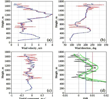
Figure 2 shows an example of wind profiles U (hk), θV(hk) and Vˆz(hk) retrieved from data measured by the Stream Line lidar on the shore of Lake Baikal, 25 Au-gust 2015 at 23:15:30 LT (local time) (here and in other fig-ures the height is above the lidar position level). For the retrieval of wind profiles in Fig. 2 we used both LSM and FSWF methods. The figure also shows the profile of the es-timate of the signal-to-noise ratio obtained from the same measurement and averaged over all the rays: SNR(hk)= M−1
M P m=1
SNR(Rˆ k, θm). It is seen from the figure that both these methods give similar results, except for a layer of 600– 900 m and a layer over 1400 m. Due to the filtration of data, the FSWF provides more smooth profiles of the wind in the layers 600–900 and 1400–1500 m than the LSM. This proves a greater effectiveness of the FSWF compared to the LSM.
The mean noise power is a function of the rangeR (Man-ninen et al., 2016). Therefore, at very low signal-to-noise ra-tios, the estimate SNR(hk)has a systematic error (in partic-ular, SNR can take negative values). This does not allow us to find an adequate threshold SNRt without the special pro-cedure of data correction (Manninen et al., 2016). To cor-rect the measured profile SNR(hk), first we use a smoothing cubic spline fit to all SNR(hk)≤0.015 and obtain the func-tion SNRs(hk)(see green squares in Fig. 2d). Then, assuming
Figure 2.Height profiles of wind velocity(a), wind direction an-gle(b)and vertical component the wind vector(c)retrieved from data measured by the Stream Line lidar, using LSM (red curves) and FSWF (blue curves);(d): height profiles of signal-to-noise ra-tio estimates SNR (black curve), SNRs (green squares) and SNRc
(green solid curve).
that at some heightshk, the true SNR is very close to zero, we find the minimum of the function SNRs(hk)and obtain a corrected profile of the signal-to-noise ratio in the form: SNRc(hk)=SNRs(hk)−min{SNRs(hk)} +SNRmin, (2) where SNRminis the unknown true minimal SNR. We note that in practice the heights of min{SNRs(hk)}and SNRmin can be different.
To avoid needing to determine SNRmin, we proceeded as follows. From our measurements from the Stream Line li-dar in Tomsk in September 2015 (focus length was 300 m; the measurements were carried out in clear weather with-out clouds) using the raw data (in binary files for correlation functions of the complex lidar signal), we obtained the fol-lowing function:
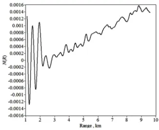
N (R)= [PN(R)−PN]/PN, (3) wherePN(R)is the mean noise power as a function of range RandPNis the noise power averaged over an interval from 1 to 3 km. An example of the functionN (R)is shown in Fig. 3. According to the figure, in the interval 1–2 km the func-tionN (R)has regular oscillations with amplitudeA∼0.001 and range periodL∼450 m (at elevation angleϕ=60◦the height periodLsinϕ–400 m).
Figure 3.FunctionN (R).
is correct, then the threshold signal-to-noise ratios can be set as SNRt=0.005 (−23 dB) in the case of FSWF and SNRt=0.01 (−20 dB) in the case of LSM. These thresh-olds are found from the profiles shown in Fig. 2a–c and de-picted in Fig. 2d as blue and red lines, respectively. In the paper of Päschke at al. (2015) the authors assert that the de-crease of the threshold SNR from 0.015 down to 0.01 would increase the data availability by almost 40 %. It corresponds to the LSM profiles presented in Fig. 2a–c. Since in the ex-periments on Lake Baikal we used the FSWF for processing the data, we could use the value SNRt=0.005−SNRmin= 0.005−0.001=0.004 as the SNR threshold. Taking into ac-count that regular oscillations of SNR of our lidar have max-imal amplitudeA∼0.001 (Fig. 3), upon obtaining the results presented below, we rejected the wind estimates that do not satisfy the following condition:
SNRs(hk)−min{SNRs(hk)} ≥0.005, (4) where information about SNRminis not required. In colour figures of this paper, the rejected estimates are shown in black.
3 Observations and analysis
The measurements were conducted over 14–28 August 2015 on the western coast of Lake Baikal (51◦50′47.17′′N, 104◦53′31.21′′E) in the area of the Baikal Astrophysical Observatory of the Institute of Solar-Terrestrial Physics SB RAS, near the Baikal Solar Vacuum Telescope (BSVT). The lidar was set at a minimum distance of 340 m from Baikal at a height of 180 m above the lake level (see Fig. 4). Accord-ing to Google Maps, the profile of the relief surface of the earth, starting from the position of the lidar and going in a northward direction up to 30 km, has 10 local maxima with heights of 180–420 m and the same number of minimums with heights of 60–250 m above the level of Lake Baikal.
Due to forest fires, the atmosphere often contained greater amounts of aerosol and, correspondingly, the lidar signal-to-noise ratio was rather high.
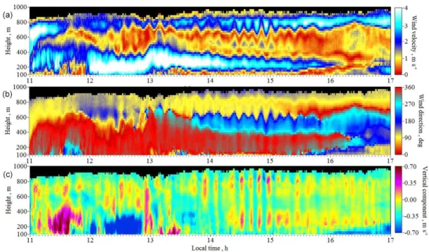
Figure 5 shows the results of lidar visualisation of the wind field during the longest observations of a gravity wave for about 4 h starting from 12:00 LT 23 August 2015. Two jet streams were observed simultaneously at heights of about 250 and 750 m a.g.l. The direction of the first jet stream (at height of 250 m) was from north to south and the direction of the other one was from east to west.
Figures 6 and 7 show the vertical profiles at 14:31 LT and temporal profiles at a height of 636.5 m a.g.l. of wind taken from data in Fig. 5. From these figures, we can clearly see oscillations of the wind speed, direction and vertical compo-nent in both height and time. They are especially evident dur-ing the period from 13:30 to 15:30 LT, when the amplitude of oscillations of the wind direction is maximal and equal to ap-proximately 45◦.
Neglecting the wind turbulence, we use the model of a plane wave for the component of the wind velocity vector Vα(subscriptα=zfor the vertical component,α=xfor the longitudinal component andα=yfor the transverse compo-nent) in the form (Vinnichenko et al., 1973):
Vα(r, t )=< Vα>+Veα(r, t ). (5) In Eq. (5)r= {z, x, y}is the radius vector in the Cartesian system with the coordinates of the centre at the lidar position, t is time,< Vα>andVeα are the regular and wave addends of theα-th component of the wind velocity, respectively. e
Vα(r, t )=Aα(z)sin
ψα(r)−2π t /Tv
(6) Aαis the wave amplitude,ψα is the wave phase andTvis the wave period. If the wind direction coincides with the direc-tion of propagadirec-tion of the internal gravity wave, thenAy=0, ψx=2π x/λvandψz=2π x/λv+π/2 (Vinnichenko et al., 1973). Here,λv is the wavelength of the wave propagating with the speedcv=λv/Tv.
Models (5) and (6) were applied to the analysis of data in Fig. 5 for a height of 766.4 m a.g.l. (inside the upper jet stream) and 47 min time interval starting from 14:20 LT, when the amplitude of wind velocity oscillations was max-imal. From these data, with allowance made for the linear trend, we found the wave addendsVeα(r, t )for the three com-ponents of the wind velocity vector. In Fig. 8, the solid curve shows the dependence ofVex on t. To determine the wave frequencyfv=1/Tv, we have used experimental function e
Vx(t )and calculated the spectral density, which is depicted in Fig. 9.
Figure 4.Map of lidar wind measurements over 14–28 August 2015.
Figure 6.Vertical profiles of the wind speed(a), the wind direction angle(b)and the vertical component of the wind vector(c)taken from the data of Fig. 4 (these profiles were measured at 14:31 LT).
Figure 7. Temporal profiles of the wind speed(a), the wind di-rection angle (b) and the vertical component of the wind veloc-ity (c) taken from the data of Fig. 5 (measurement height of 636.5 m).
Figure 8.Time dependence of the wave addend of the longitudi-nal wind velocity: (solid curve) measurements by the Stream Line lidar starting from 14:20 LT on 23 August 2015 at a height of 766.4 m a.g.l. (the data of Fig.5a were used); (dashed curve) result of least-squares fitting of sine-wave dependence (6) for the wave addendVex(t )to the measured data shown by the solid curve.
Figure 9.Normalised spectrum of the wave addend of wind velocity calculated from the data shown by the solid curve in Fig. 8.
amplitudeAx. The amplitude of wave addend for the longi-tudinal component of the wind velocity vector turned out to be 0.96 m s−1. The model temporal profileVex(t )calculated by Eq. (6) with the use of experimental values ofAx,ψxand Tvis shown as a dashed curve in Fig. 8.
Parameters of the wave addend of the vertical wind veloc-ityVez(t )were found in the same way. The estimates of pe-riods of the internal wave for the longitudinal and vertical components coincided fully (Tv=9 min), amplitude Az= 0.3 m s−1 is approximately 3 times smaller than the ampli-tude of wave addend of the longitudinal component of the wind velocity vector andψz−ψx=π/2. Since the amplitude Ay6=0 (see Figs. 5b and 7b), the direction of propagation of the internal wave did not coincide with the wind direction.
Figure 10.Spatio-temporal distribution of the wind velocity(a)and the time profile of the wind velocity at a height of 532.6 m a.g.l.(b) ob-tained from measurements by the Stream Line lidar on 20 August 2015.
Figure 11. Spatio-temporal distributions of the wind speed(a), wind direction angle(b), vertical component of the wind vector(c)and signal-to-noise ratio(d)obtained from measurements of the Stream Line lidar on 14 August 2015 starting from 19:24 LT.
filtration (see Sect. 2) the instrumental error of the wind ve-locity estimate, obtained atM=180 and with a SNR thresh-old 0.005 (Eq. 4), does not exceed 0.1 m s−1. In our exper-iment for heights h< 500 m a.g.l., it did not usually exceed 0.05 m s−1. For the vertical wind component the instrumen-tal error is approximately 3 times smaller.
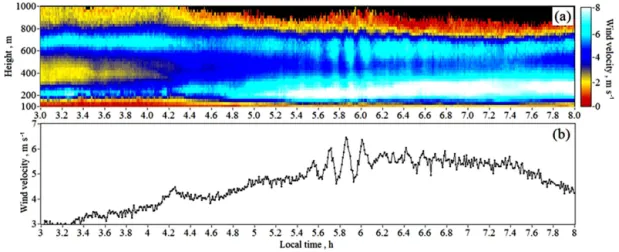
Figures 5–7 illustrate the long time AIW in the case of weak wind, when wind velocity averaged over the periodTv is 1–2.5 m s−1. Figure 10a shows an example of the spatio-temporal distribution of wind velocity, where the atmo-spheric internal wave was observed since 05:30 LT for about 40 min and the averaged wind velocity was about 5.5 m s−1. According to the data in Fig. 10b, the period and amplitude
of the wave were, respectively, 9 min and 0.9 m s−1. Two jet streams were also observed for 5 h; one at a height of approx-imately 200 m a.g.l. and another at a height of 500 m a.g.l. and higher.
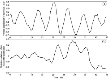
Figure 11 depicts the spatio-temporal distributions of wind and the signal-to-noise ratio in the evening of 14 August for about 45 min. Here we see one jet stream at a height ∼730 m a.g.l. and an atmospheric internal wave. In the layer of 100–500 m a.g.l., the oscillations of the wind speed, di-rection and vertical component are accompanied by periodic variations of the signal-to-noise ratio SNR. It is known that SNR is proportional to the attenuated backscatter coefficient e
coefficient at rangeRandβtis the radiation extinction coef-ficient due to absorption and scattering by air molecules and aerosol particles. For rangeR≤250 m, the effect of turbulent pulsations of the refractive index of air on the intensity of the laser beam focused at a distance of 800 m (see Table 2) can be neglected. Therefore, for such ranges, the SNR also does not depend on turbulent pulsations of the refractive index. We used the data of Fig. 11d for a height of 220.8 m ag.l. and calculated the relative variations of the attenuated backscatter coefficientη(t )= [βeπ(t )−<βeπ>T]/ <βeπ>T as
η(t )= [SNR(t )−<SNR>T]/ <SNR>T, (7) where the operator < . . .>T denotes the time averaging for the period of 45 min.
Since the SNR oscillates within the height (a.g.l.) range 100–500 m in Fig. 11d, it is evident, that the backscatter coefficient eβπ should vary with time too. These attenuated backscatter coefficient (SNR) variations can be caused by os-cillations of the vertical component of the wind velocity vec-tor, with a relatively high amplitude. To test it, we compared Vz(t )withη(t ).
Figure 12 shows the temporal profilesVz(t )andη(t ) ob-tained from the data depicted in Fig. 11 for a height of 220.8 m a.g.l. From the analysis of the curve in Fig. 12a, it follows that the period of oscillationsTvof the vertical com-ponent of wind velocity is 6.5 min. The same period of os-cillations is also observed for other components of the wind vector, with a phase that is shifted by 90◦about the phase of
e
Vz(t ). According to Fig. 12b,η(t )is characterised not only by periodic variations with time, but also by non-stationarity within the considered time interval. It follows from the rough estimates that the period of oscillations of the backscatter co-efficient is close toTv=6.5 min, while the phase is shifted by 90 degrees about the phase ofVez(t ).
In addition to these three cases of AIW occurrence, we succeeded in observing this phenomena 3 times more for the period of measurements. Thus, on 25 August before dawn (04:30–05:06 LT), two jet streams and AIW with the period Tv≈9 min and the amplitude Ax≈1 m s−1 at a height of 402.7 m a.g.l. were observed in the atmospheric boundary layer. The next day (26 August 2015), the internal wave with the period Tv≈18 min and the amplitude Ax≈0.7 m s−1 at the same height 402.7 m a.g.l., passed from 16:22 to 19:00 LT. On the same day, the AIW with the halved pe-riod (Tv≈9 min) and the amplitude Ax≈0.4 m s−1 at the height 402.7 m a.g.l. was observed 50 min later from 19:50 to 20:35 LT.
4 Summary
Thus, the results of the experimental campaign in the coastal zone of Lake Baikal on August 2015 show that the raw data from measurements by the Stream Line lidar allow us to vi-sualise the spatio-temporal structure of the wind field in the
Figure 12.Time dependence of the vertical component of the wind vector(a)and relative variations of the attenuated backscatter coef-ficient(b)obtained from the data depicted in Fig. 11c, d at a height of 220.8 m a.g.l.
atmospheric boundary layer and reveal the presence of low-level jet streams and atmospheric internal waves. The distin-guishing feature of the atmospheric conditions of the Lake Baikal is the occurrence of the stable thermal stratification in the ABL during the daytime. The low-level jet streams were observed during day and night while none of the AIWs events were observed at night-time.
A total of six cases of AIW formation have been revealed, which always occurred in the presence of one or two (in five out of six cases) narrow jet streams at heights of about 200 and 700 m a.g.l. When two jet streams were formed, the period of oscillations of the wave addend of the wind vec-tor components was 9 min. In only one case it was about 18 min. In the presence of a single jet stream (at a height of 730 m a.g.l.), the period of oscillations of the wind vector components during AIW was about 6.5 min. The amplitude of oscillations of the horizontal wind components was most often about 1 m s−1, while the amplitude of oscillations of the vertical velocity was 3 times smaller. In most cases, the internal waves were observed for 45 min (5 oscillations with the periodTv=9 min). Only once the lifetime of the atmo-spheric internal wave was about 4 h.
5 Data availability
All the data presented in this study are available from the authors upon request.
This study was supported by the Russian Science Foundation, Project No. 14-17-00386.
Edited by: M. Kulie
Reviewed by: two anonymous referees
References
Banakh, V. A., Brewer, V. A., Pichugina, E. L., and Sma-likho, I. N.: Measurements of wind velocity and di-rection with coherent Doppler lidar in conditions of a weak echo signal, Atmos. Oceanic Optics, 23, 381–388, doi:10.1134/S1024856010050076, 2010.
Banakh, V. and Smalikho, I.: Coherent Doppler Wind Lidars in a Turbulent Atmosphere, Artech House Publishers, ISBN-13: 978-1-60807-667-3, 2013.
Banakh, V. A., Smalikho, I. N., Falits, A. V., Belan, B. D., Arshinov, M. Y., and Antokhin, P. N.: Joint radiosonde and Doppler lidar measurements of wind in the boundary layer of the atmosphere, Atmos. Oceanic Optics, 28, 185–191, doi:10.1134/S1024856015020025, 2015.
Baumgarten, G., Fiedler, J., Hildebrand, J., and Lübken, F.-J.: In-ertia gravity wave in the stratosphere and mesosphere observed by Doppler wind and temperature lidar, Geophys. Res. Lett., 42, 10929–10936, doi:10.1002/2015GL066991, 2015.
Benediktov, E. A., Belikovich, V. V., Bakhmet’eva, N. V., and Tol-macheva, A. V.: Seasonal and daily variations of the velocity of vertical motions at altitudes of the mesosphere and lower ther-mosphere near Nizhny Novgorod, Geomagn. Aeron., 37, 88–94, 1997.
Chouza, F., Reitebuch, O., Jähn, M., Rahm, S., and Weinzierl, B.: Vertical wind retrieved by airborne lidar and analysis of island in-duced gravity waves in combination with numerical models and in situ particle measurements, Atmos. Chem. Phys., 16, 4675– 4692, doi:10.5194/acp-16-4675-2016, 2016.
Chunchuzov, I., Vachon, P., and Li, X.: Analysis and modeling of atmospheric gravity waves observed in Radarsat SAR images, Remote Sens. Environ., 74, 343–361, 2000.
German, M. A.: Space Methods of Investigation in Meteorology, Gidrometeoizdat Publishers, 1985 (in Russian).
Kozhevnikov, N. N.: Perturbations of the atmosphere at a flow around mountains, Nauchnyi Mir Publishers, ISBN-13: 5-89176-059-2, 1999 (in Russian).
Li, X., Zheng, Q., Pichel, W. G., Yan, X.-H., Liu, W. T., and Clemente-Colon, P.: Analysis of coastal lee waves along the coast of Texas observed in advanced very high resolu-tion radiometer images, J. Geophys. Res., 106, 7017–7025, doi:10.1029/1999JC000019, 2001.
Lyulyukin, V. S., Kallistratova, M. A., Kouznetsov, R. D., Kuznetsov, D. D., Chunchuzov, I. P., and Chirokova, G. Y.: Inter-nal gravity-shear waves in the atmospheric boundary layer from acoustic remote sensing data, Izv. Atmos. Ocean. Phys., 51, 193– 202, 2015.
Makarenko, N. I. and Maltseva, J. L.: Interference of lee waves over mountain ranges, Nat. Hazards Earth Syst. Sci., 11, 27–32, doi:10.5194/nhess-11-27-2011, 2011.
Manninen, A. J., O’Connor, E. J., Vakkari, V., and Petäjä, T.: A gen-eralised background correction algorithm for a Halo Doppler
li-dar and its application to data from Finland, Atmos. Meas. Tech., 9, 817–827, doi:10.5194/amt-9-817-2016, 2016.
Newsom, R. K. and Banta, R. M.: Shear-flow instability in the stable nocturnal boundary layer as observed by Doppler lidar during CASES-99, J. Atmos. Sci., 60, 16–33, 2003.
O’Connor, E. J., Illingworth, A. J., Brooks, I. M., Westbrook, C. D., Hogan, R. J., Davies, F., and Brooks, B. J.: A Method for esti-mating the turbulent kinetic energy dissipation rate from a ver-tically pointing Doppler lidar, and independent evaluation from balloon-borne in situ measurements, J. Atmos. Ocean. Tech., 27, 1652–1664, doi:10.1175/2010JTECHA1455.1, 2010.
Päschke, E., Leinweber, R., and Lehmann, V.: An assessment of the performance of a 1.5 µm Doppler lidar for operational vertical wind profiling based on a 1-year trial, Atmos. Meas. Tech., 8, 2251–2266, doi:10.5194/amt-8-2251-2015, 2015.
Pearson, G., Davies, F., and Collier, C.: An Analysis of the Per-formance of the UFAM Pulsed Doppler Lidar for Observing the Boundary Layer, J. Atmos. Ocean. Tech., 26, 240–250, doi:10.1175/2008JTECHA1128.1, 2009.
Plougonven, R. and Zhang, F.: Internal gravity waves from atmospheric jets and fronts, Rev. Geophys., 52, 33–76, doi:10.1002/2012RG000419, 2014.
Román-Cascón, C., Yagüe, C., Mahrt, L., Sastre, M., Steeneveld, G.-J., Pardyjak, E., van de Boer, A., and Hartogensis, O.: In-teractions among drainage flows, gravity waves and turbulence: a BLLAST case study, Atmos. Chem. Phys., 15, 9031–9047, doi:10.5194/acp-15-9031-2015, 2015.
Sathe, A. and Mann, J.: Measurement of turbulence spectra using scanning pulsed wind lidars, J. Geophys. Res., 117, D01201, doi:10.1029/2011JD016786, 10329–10330, 2012.
Smalikho, I.: Techniques of wind vector estimation from data mea-sured with a scanning coherent Doppler lidar, J. Atmos. Ocean. Tech., 20, 276–291, 2003.
Smalikho, I. N. and Banakh, V. A.: Estimation of air-craft wake vortex parameters from data measured with a 1.5 µm coherent Doppler lidar, Opt. Lett., 40, 3408–3411, doi:10.1364/OL.40.003408, 2015a.
Smalikho, I. N. and Banakh, V. A.: Estimation of aircraft wake vortex parameters from data measured by a Stream Line lidar, in: Proceedings of SPIE 21st International Symposium “Atmo-spheric and Ocean Optics: Atmo“Atmo-spheric Physics”, 9680, 968037-1–968037-7, doi:10.1117/12.2205281, 2015b.
Smalikho, I. N., Banakh, V. A., Falits, A. V., and Rudi, Y. A.: Determination of turbulence energy dissipation rate from data measured by the Stream Line lidar in the atmo-spheric surface layer, Atmos. Oceanic Optics, 28, 980–987, doi:10.15372/AOO20151006, 2015a (in Russian).
Smalikho, I. N., Banakh, V. A., Holzäpfel, F., and Rahm, S.: Estima-tion of aircraft wake vortex parameters from the array of radial velocities measured by a coherent Doppler lidar, Atmos. Oceanic Optics, 28, 742–750, doi:10.15372/AOO20150801, 2015b (in Russian).
Smalikho, I. N., Banakh, V. A., Holzäpfel, F., and Rahm, S.: Method of radial velocities for the estimation of aircraft wake vortex pa-rameters from data measured by coherent Doppler lidar, Opt. Ex-press, 23, A1194–A1207, doi:10.1364/OE.23.0A1194, 2015c. Spiridonov, Y. G., Pichugin, A. P., and Shestopalov, V. P.: Space
Sun, J., Nappo, C. J., Mahrt, L., Beluši´c, D., Grisogono, B., Stauf-fer, D. R., Pulido, M., Staquet, C., Jiang, Q., Pouquet, A., Yagüe, C., Galperin, B., Smith, R. B., Finnigan, J. J., Mayor, S. D., Svensson, G., Grachev, A. A., and Neff, W. D.: Review of wave-turbulence interactions in the stable atmospheric boundary layer, Rev. Geophys., 53, 956–993, doi:10.1002/2015RG000487, 2015. Vakkari, V., O’Connor, E. J., Nisantzi, A., Mamouri, R. E., and Had-jimitsis, D. G.: Low-level mixing height detection in coastal lo-cations with a scanning Doppler lidar, Atmos. Meas. Tech., 8, 1875–1885, doi:10.5194/amt-8-1875-2015, 2015.
van Dinther, D., Wood, C. R., Hartogensis, O. K., Nordbo, A., and O’Connor, E. J.: Observing crosswind over urban terrain using scintillometer and Doppler lidar, Atmos. Meas. Tech., 8, 1901– 1911, doi:10.5194/amt-8-1901-2015, 2015.
Vel’tishchev, N. F. and Stepanenko, V. M.: Mesometeorological Processes, Moscow State University Publishers, ISBN-13: 978-5-89575-118-3, 2006 (in Russian).
Vinnichenko, N. K., Pinus, N. Z., Shmeter, S. M., and Shur G. N.: Turbulence in the Rree Atmosphere, edited by: Dutton, J. A., Consultants Bureau, 262 pp., ISBN-13: 978-1-4757-0100-5, 1973.