KamLAND Data and the Solution to the Solar Neutrino Problem
P. C. de Holanda
1and A. Yu. Smirnov
2 ,31
Instituto de F´ısica Gleb Wataghin - UNICAMP, 13083-970 Campinas SP, Brazil
2
The Abdus Salam International Centre for Theoretical Physics, I-34100 Trieste, Italy
3
Institute for Nuclear Research of Russian Academy of Sciences, Moscow 117312, Russia
Received on 17 November, 2003
The first KamLAND results are in a very good agreement with the predictions made on the basis of the solar neutrino data and the LMA realization of the MSW mechanism. We perform a combined analysis of the KamLAND (rate, spectrum) and the solar neutrino data with a free boron neutrino fluxfB. The best fit values of neutrino parameters are∆m2
= 7.1·10−5 eV2,tan2θ = 0.40andfB = 1.04with the1σintervals:
∆m2 = (6
.4−8.4)·10−5eV2,tan2θ = 0.33−0.48. We find the3σupper bounds:∆m2
<1.7·10−4
eV2
andtan2
θ < 0.64, and the lower bound∆m2
> 4.8·10−5 eV2. In the best fit point we predict for
SNO: CC/NC= 0.32+0.08
−0.07andA
SN O
DN = 3.0±0.8%(68% C.L.), andA SN O
DN <6%at the3σlevel. Further
improvements in the determination of the oscillation parameters are discussed and implications of the solar neutrino and KamLAND results are considered.
1
Introduction
The first KamLAND results [1] are the last (or almost last) step in resolution of the long-standing solar neutrino problem [2]. In fact, KamLAND excludes also all non-oscillationsolutions based on neutrino spin-flip in the mag-netic fields of the Sun, on the non-standard neutrino interac-tions, etc.. More precisely, KamLAND excludes them as the dominant mechanisms of the solar neutrino conversion.
By the time of the KamLAND announcement, the so-lar neutrino data [3-10] have definitely selected LMA as the most favorable solution based on neutrino mass and mi-xing [11-13]. After the publication of KamLAND results, SNO experiment published their results on the salt phase detection [14], confirming LMA predictions and restricting even more the allowed region for neutrino parameters. The best fit point from the free boron neutrino flux fit [15] is
∆m2 = 6.31·10−5eV2 tan2θ = 0.39
fB = 1.06, (1)
wherefB ≡ FB/FBSSM is the boron neutrino flux in the
units of the Standard Solar Model predicted flux [16]. On basis of the solar neutrino results (and the assump-tion of the CPT invariance) predicassump-tions for the KamLAND experiment have been calculated. A significant suppression of the signal was expected in the case of the LMA solution. The predicted ratio of the numbers of events with the visi-ble (prompt) energies,Ep, above 2.6 MeV with and without
oscillations equals [13]: RLM A
KL = 0.65
+0.08
−0.38 (3σ). (2) For other solutions of the solar neutrino problem one expec-tedRKL= 0.9−1, where the deviation from 1 can be due
to the effect of nonzero 1-3 mixing.
In the best fit point (1) the predicted spectrum has (i) a peak atEp ≈ (3.0−3.6) MeV, (ii) a suppression of the
number of events near the threshold energyEp ≈2.6MeV
and (iii) a significant suppression of the signal (with respect to the no-oscillation case) at the high energies:Ep>(4−5)
MeV [13]. No distortion of the spectrum is expected for the other solutions.
The first KamLAND results, both the total number of events and spectrum shape [1], are in a very good agreement with predictions:
RexpKL= 0.611±0.094. (3) The spectral data (although not yet precise) reproduce well the features described above. As a result, the allowed “is-land” in the ∆m2 −sin2
2θ plane with the best fit Kam-LAND point covers the best fit point from the solar neutrino analysis [1].
This work is based in our recent paper [17, 15] where the KamLAND data were analysed, as well as the combination of this analysis with solar neutrinos data.
2
KamLAND
The KamLAND (Kamioka Liquid scintillator Anti-Neutrino Detector) experiment detects anti-neutrinos created in∼26 nuclear reactors situated around the detector site, tipically at distances between 80 and 200 Km. It consists of a very large volume scintilator detector, that can detect the anti-neutrinos from the inverse beta-decay reaction:
¯
In a given energy bina(a= 1, ....13)the signal at Kam-LAND is determined by
Na=A X
i
Z Ea+∆E
Ea
dEp Z
dE′
pPiFiσf(Ep, Ep′), (4)
where∆E= 0.425MeV, Pi=
µ
1−sin22θ12sin2∆m 2 12Li
4E
(5) is the vacuum oscillation survival probability for ireactor situated at the distanceLi from KamLAND,Fiis the flux
fromireactor,σis the cross-section ofνp¯ →e+n
reaction, Ep is the observed prompt energy, Ep′ is the true prompt
energy,f(Ep, Ep′)is the energy resolution function,Ais the
factor which takes into account the fiducial volume, the time of observation, etc.. We sum over all reactors contributing appreciable to the flux at KamLAND.
The suppression factor of the total number of (reactor neutrino) events above certain threshold is defined as:
RKL(∆m2,tan2θ)≡
N(∆m2,tan2θ)
N0 , (6)
whereN =P
aNa,Na is given in (4) andN0is the total
number of events in the absence of oscillations (following KamLAND we will callN andN0the rates).
1). KamLAND spectrum.The KamLAND data are analyzed through a Poisson statistics, using the followingχ2:
χ2= X
i=1,13
2
·
Nth
i −Niobs+Niobsln
µ
Nobs i Nth
i ¶¸
where the lnterm is absent in bins with no events (5 last bins).
We find that forEp ≥2.6MeV the minimum ofχ2spec
is achieved for
∆m2= 7.2·10−5
eV2, tan2θ= 0.52, (7) and in this pointχ2/d.o.f. = 5.91/11. Notice that in con-trast with the KamLAND result [1] our best fit mixing devi-ates from the maximal mixing.
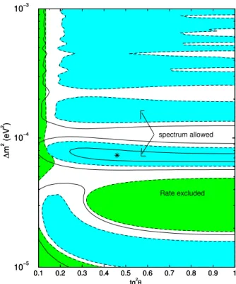
We present in Fig. 1 the contours of constant confi-dence level with respect to the best fit point (7) in the (∆m2−tan2θ)
plane using relation: χ2 =χ2
min+ ∆χ
2 , where∆χ2 = 1,3.84
and6.63for1σ,95%and99%C.L. correspondingly.
The contours manifest an oscillatory pattern in∆m2in spite of a strong averaging effect which originates from large spread in distances from different reactors. The pattern can be described in terms of oscillations with certain effective distance,Lef f, and effective oscillation phaseφef f:
φef f =
∆m2 12Lef f
4E , Lef f ≈165 km. (8) Lef f corresponds to the distance between KamLAND and
the closest set of reactors which provides the large fraction of the antineutrino flux.
0.1 0.2 0.3 0.4 0.5 0.6 0.7 0.8 0.9 1 0.1 0.2 0.3 0.4 0.5 0.6 0.7 0.8 0.9 1
tg2θ 10−5
10−4 10−3
∆
m
2 (eV 2 )
0.1 0.2 0.3 0.4 0.5 0.6 0.7 0.8 0.9 1 tg2θ
10−5 10−4 10−3
∆
m
2 (eV 2 )
Rate excluded spectrum allowed
Figure 1. The KamLAND spectrum analysis forEp >2.6MeV. Shown are the allowed regions of oscillation parameters at 68% (inner solid lines), 95% (grey) and 99% C.L. (outer solid lines). The best fit point is indicated by star. Also shown are the regions excluded by the rate analysis at95%C.L. (dark).
Let us consider the 95% allowed regions.
(i) The lowest “island” allowed by KamLAND with ∆m2 <2·10−5eV2 corresponds to the oscillation phase φef f < π/2. This region is excluded by the absence of
significant day-night asymmetry of the Super-Kamiokande signal. In this domain, the predicted asymmetry at SNO, ASN O
DN >17%, is still consistent with data.
(ii) The second allowed region,∆m2= (5−10)·10−5 eV2, corresponds to the first oscillation maximum,φef f ∼ π(maximum of the survival probability). It contains the best fit point.
(iii) The third island is at∆m2= (13−23)·10−5eV2: it corresponds to the oscillation maximum (second maximum of the survival probability) withφef f ∼2π.
There is a continuum of the allowed regions above ∆m2 ∼ 3·10−4 eV2. The third region merges with the continuum at 99% CL.
At the1σlevel the second island is the only allowed re-gion.
2) KamLAND rate.In Fig. 1 we show the regions excluded by the KamLAND rate at95%C.L.. The borders of these regions coincide with contours of constantRmax
KL = 0.80
andRmin
KL = 0.42obtained in [13]). The exclusion region
signal is too strong. Another region of significant suppres-sion (second oscillation minimum withφef f = 3π/2) is at
∆m2∼(9−12)·10−5eV2.
3). KamLAND spectrum and rate. Following procedure in [1] we have performed also combined analysis of spectrum and rate introducing the free normalization parameter of the spectrum,RKL, and defining theχ2as
χ2
spec,R=χ2spec+χ2R, (9)
where
χ2
R=
µR
KL−0.611
0.094
¶2
. (10)
We find results which are very close to those from our spec-trum analysis. In particular, the best fit value of mixing is tan2θ= 0.48
and∆m2= 7.31·10−5 eV2.
As it follows from our consideration here, the values of oscillation parameters extracted from the KamLAND data, (∆m2, tan2θ)
KL, are in a very good agreement
with the values from independent solar neutrino analysis (∆m2, tan2θ)
sun. For the best fit points (1), (7) we
con-clude that within1σ(see Fig. 1) (∆m2, tan2θ)
KL= (∆m2, tan2θ)sun. (11)
At the same time, the data do not exclude that the solar and KamLAND parameters are different, and moreover, the dif-ference still can be large. For instance,(∆m2, tan2θ)
KL
can coincide with the present best fit point or be in the high ∆m2island, whereas(∆m2, tan2θ)
sun can be at lower
∆m2.
3
Solar Neutrinos
We use the same data set and the same procedure of analysis as in our previous publication [15]. Here the main ingredi-ents of the analysis are summarized.
The data sample consists of
- 3 total rates: (i) theAr-production rate,QAr, from
Homes-take [3], (ii) theGe−production rate,QGefrom SAGE [5]
and (iii) the combinedGe−production rate from GALLEX and GNO [6];
- 44 data points from the zenith-spectra measured by Super-Kamiokande during 1496 days of operation [7];
- 34 day-night spectral points from SNO [9, 10]. - CC, NC and ES rates from SNO salt-phase [14]
Altogether the solar neutrino experiments provide us with 84 data points. The SNO salt phase data were issued after the publication of the first KamLAND data analyzed here. Nevertheless we included it in our solar scenario since they have an important role in discriminating the∆m2
de-generacy that arises from KamLAND analysis.
All the solar neutrino fluxes, but the boron neutrino flux, are taken according to SSM BP2000 [16]. The bo-ron neutrino flux is treated as a free parameter. For the hep−neutrino flux we take fixed valueFhep = 9.3×10³
cm−2 s−1
[16, 18].
Thus, in our analysis of the solar neutrino data as well as in the combined analysis of the solar and KamLAND results we have three fit parameters:∆m2,tan2θandf
B.
We define the contribution of the solar neutrino data to χ2
as
χ2sun=χ 2
rate+χ
2
SK+χ
2
SN O+χ
2
SN O−II, (12)
whereχ2
rate,χ2SK,χ2SN Oandχ2SN O−II are the
contributi-ons from the total rates, the Super-Kamiokande zenith spec-tra, the SNO day and night spectra and the SNO salt phase correspondingly. The main result of analysis performed in [15] is given here in Eq. (1).
4
Solar neutrinos and KamLAND
We have performed two different combined fits of the data from the solar neutrino experiments and KamLAND.
1) KamLAND rate and solar neutrino data. There are 84 (solar) + 1 (KamLAND) data points - 3 free parameters = 82 d.o.f.. We define the globalχ2
for this case as
χ2sun,R=χ
2
sun+χ
2
R, (13)
whereχ2
sun and χ
2
R are given in (12) and (10). The
mi-nimumχ2
sun,R(min)/d.o.f. = 67.2/82corresponds to the
C.L. = 88% . It appears at
∆m2 = 5.58
·10−5eV2 tan2θ = 0.39
fB = 1.08. (14)
This point practically coincides with what we have obtained from the solar neutrino analysis only.
We construct the contours of constant confidence le-vel in the (∆m2 −tan2θ) plot using the following pro-cedure. We perform minimization of χ2
sun,R with respect
tofB for each point of the oscillation plane, thus getting χ2
sun,R(∆m2,tan
2θ). Then the contours are defined by the
condition χ2
sun,R(∆m
2,tan2θ) = χ2
sun,R(min) + ∆χ
2 , where∆χ2= 2.3,4.61,5.99, 9.21
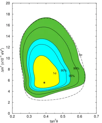
0.2 0.3 0.4 0.5 0.6 0.7 tan2θ
0 2 4 6 8 10 12 14 16 18 20
∆
m
2 (x10
−5
eV
2 )
1σ 90% 95%
99% 3σ
Figure 2. The allowed regions intan2
θ−∆m2plane from a com-bined analysis of the solar neutrino data and the KamLAND rate, at 1σ, 90%, 95%, 99% and 3σC.L.. The best fit point is marked by star. Also shown in dashed lines the allowed region at 99% C.L. with only solar data.
According to the figure, the main impact of the Kam-LAND rate is strengthening of bound on the allowed region from below due to strong suppression of the KamLAND rate at∆m2 = (2−5)·10−5eV2(see Fig. 1) - region of the first oscillation minimum in KamLAND. The lines of cons-tant confidence level are shifted to larger∆m2. The Kam-LAND rate leads to a distortion (shift to smaller mixings) of contours at∆m2∼10−4eV2where the second oscillation minimum at KamLAND is situated. The upper part of the allowed region is modified rather weakly.
2). KamLAND spectrum and solar neutrino data.We calcu-late
χ2
global=χ
2
sun+χ
2
spec, (15)
where χ2
spechas been defined in (2). In this case we have
84 (solar) + 13 (KamLAND) data points - 3 free parameters = 94 d.o.f.. The absolute minimum, χ2
global(min) = 73.4
(which corresponds to a very high confidence level: 94%), is at
∆m2 = 7.13·10−5eV2 tan2θ = 0.40
fB = 1.038. (16)
The best fit value of∆m2is slightly higher than that from the solar data analysis. The solar neutrino data have higher sensitivity to mixing, whereas the KamLAND is more sen-sitive to∆m2, as a result, in (16) the value of∆m2is close to the one determined from the KamLAND data only (7),
0.2 0.3 0.4 0.5 0.6 0.7
tan2θ
0 2 4 6 8 10 12 14 16 18 20
∆
m
2 (x10 −5 eV 2 )
1σ 90% 95%99% 3σ
Figure 3. The allowed regions intan2
θ−∆m2
plane, from a combined analysis of the solar neutrino data and the KamLAND spectrum at 1σ, 90%, 95%, 99% and 3σC.L.. The best fit point is marked by star.
whereas tan2θ almost coincides with mixing determined from the solar neutrino results (1).
We construct the contours of constant confidence levels in the oscillation plane, similarly to what we did for the fit of the solar data and the KamLAND rate (Fig. 3).
As compared with the solar data analysis, KamLAND practically has not changed the upper bound on mixing or ∆m2. At the3σlevel we get:
∆m2>4.8·10−5eV2
, tan2θ <0.64, 99.73% C.L. . (17) The spectral data disintegrate the LMA region. At the3σ level only a small spot is left in the range∆m2>1.2·10−4 eV2.
The region “splits” into two regions, above and below ∆m2>1.2·10−4eV2, which we will refer to as the lower (l-) and higher (h-) LMA regions. (Existence of these two regions can be seen already from an overlap of the solar and KamLAND allowed regions in [1]).
The shrink in allowed region around ∆m2 ∼ 1.2 · 10−4eV2 corresponds to the second oscillation minimum (φef f ∼3π/2) atEp∼(3−4)M eV which contradicts the
spectral data.
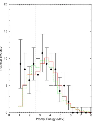
0 1 2 3 4 5 6 7 8 Prompt Energy (MeV)
0 5 10 15 20
Events/0.425 MeV
Figure 4. The expected prompt energy spectra for the best fit points from the l-region (solid histogram) and h-region (dashed histo-gram). Also shown are the KamLAND experimental points.
well understood in terms of the effective oscillation phase
φef f:
N(Ep)∼N0(Ep)£1 +D(Ep) sin2φef f¤, (18) whereD(Ep)is the averaging factor.
In the best fit point of l-region (16), the peak atEp≈3.6 MeV corresponds to the oscillation maximum φef f = π (exact position of maximum of the survival probability is at
Ep = 4.3MeV). The closest oscillation minimum (phase
φef f = 3π/2) is atEp ≈2.4MeV and the next maximum (φef f = 2π) is atEp ≈1.8MeV. Due to strong averaging effect the structures below (inEp) the main maximum are not profound and look more like a shoulder below the peak. The first oscillation minimum is atEp= 7.2MeV.
The measured spectrum, indeed, gives a hint of existence of the low energy shoulder. Evidently with the present data it is impossible to disentangle the l- and h- spectra. Substantial decrease of errors is needed. Also decrease of the energy th-reshold will help. According to Fig. 4,Nl(Ep)> Nh(Ep) atEp > 3.5MeV, andNl(Ep) < Nh(Ep)at lower ener-gies, especially in the intervalEp= (2.0−2.5)MeV. The-refore for the low threshold the difference betweenNl(Ep) andNh(Ep)can not be eliminated by normalization (mixing angle).
For convenience, the results of different fits are summa-rized in the Table 1. It shows high stability of the extracted parameters with respect to a type of analysis.
5
Next step
The key problems left after the first KamLAND results are • more precise determination of the neutrino
parame-ters: in particular, (i) precise determination of the deviation of 12-mixing from maximal mixing, (ii) strengthening of the upper bound on∆m2
(iii) dis-crimination between the two existing regions; • searches for effects beyond the single∆m2
and single mixing approximation;
• searches for differences of the neutrino oscillation pa-rameters determined from KamLAND and from the solar neutrino experiments.
Notice that precise knowledge of the parameters is cru-cial not only for the neutrinoless double beta decay sear-ches, long baseline experiments, studies of the atmospheric and supernova neutrinos, etc., but also for understanding of physics of the solar neutrino conversion. In the region of the best fit point a dominating process (at least forE >(0.5−1)
MeV) is the adiabatic neutrino conversion (MSW), whereas in the high∆m2region allowed by KamLAND at the2σ le-vel, the effect is reduced to the averaged vacuum oscillations (a la Gribov-Pontecorvo) [19] with small matter corrections.
In this connection, we will discuss two questions. How small∆m2
can be?This is especially important ques-tion,e.g., for measurements of the earth regeneration effect. In the l-region we get
∆m2>4.8
·10−5 eV2, (3σ)
(19) and it is difficult to expect that lower values will be allowed. The bound (19) appears as an interplay of both the KamLAND rate and the shape. As it follows from the Fig. 2, the KamLAND rate strengthens the lower bounds:
∆m2 ≥ (2.7, 3.7, 4.5)×10−5
eV2, at the 1σ, 2σ, 3σ
correspondingly which should be compared with ∆m2 ≥
(2.2, 2.9, 3.8)×10−5
eV2 from the solar analysis only. Adding the spectral data results in the bounds ∆m2 ≥
4.8, 5.6, 6.2 ×10⁻⁵eV2
With decrease of ∆m2 the oscillatory pattern of the spectrum shifts to lower energies. For∆m2= 5·10−5eV2 the maximum of spectrum is atEp= 2.7MeV and the oscil-lation suppression increases with energy [13]. The oscilla-tion minimum is atEp≈5MeV. IfRKL(2.7 MeV) = 0.81, then RKL(4.0 MeV) = 0.47. The KamLAND spectrum does not show such a fast decrease.
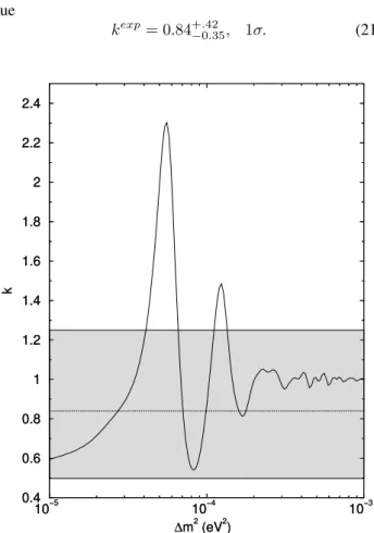
One can characterize the spectrum distortion by a rela-tive suppression of signal at the high (say, above 4.3 MeV) and at the low (below 4.3 MeV) energies The energy in-terval (2.6 - 4.3) MeV contains KamLAND energy 4 bins. Introducing the suppression factorsRKL(<4.3 MeV)and
RKL(>4.3 MeV)we can define the ratio
k=1−RKL(>4.3 MeV) 1−RKL(<4.3 MeV)
kwhich we will call theshape parameterdoes not depend on the mixing angle and normalization of spectrum. It in-creases with increase of the oscillation suppression at high energies.
Using the KamLAND data we get the experimental va-lue
kexp= 0.84+.42
−0.35, 1σ. (21)
10−5 10−4 10−3
∆m2 (eV2) 0.4
0.6 0.8 1 1.2 1.4 1.6 1.8 2 2.2 2.4
k
10−5 10−4 10−3
∆m2 (eV2) 0.4
0.6 0.8 1 1.2 1.4 1.6 1.8 2 2.2 2.4
k
Figure 5. The dependence of the shape parameter k on ∆m2 . Shown are the central experimental value (dotted line) and the1σ
experimental band (shadowed).
In Fig. 5 we present the dependence of the shape pa-rameter k on∆m2. For the spectrum which corresponds to the best combined fit we find k = 0.70, whereas for ∆m2 = 5·10−5 eV2 the ratio equals k = 2.0. For the h-region best point:k= 1.2.
Notice that in the l-region below∆m2= 8·10−5eV2, kincreases quickly with decrease of∆m2, reaching a ma-ximal value at ∆m2 = 5.5 ·10−5 eV2. Below that, the parameterkdecreases with∆m2. In this region, however, the total event rate decreases fast giving the bound on∆m2. This explains a shift of the allowed (at3σ) region to smaller mixings with decrease of∆m2.
Notice also that the central experimental value ofkcan be reproduced in the both allowed regions (l- and h-). The-refore future precise measurement of spectrum will further sharpen determination of∆m2
within a given island. To dis-criminate among the islands one needs to use more elabora-ted criteria (not justk) or a complete spectral information.
How large is the large mixing? In contrast to [1] our best fit point is at non-maximal mixing(sin22θ = 0.86)
being rather close to the best fit point from the solar neutrino
analysis. Similar deviation from maximal mixing has been obtained in our rate+spectrum analysis. Notice that the KamLAND data have weak sensitivity to the mixing (wea-ker than the solar neutrino data). The allowed regions cover the interval
tan2θ= 0.12−1.00 (θ < π/2), 95%C.L.. (22)
Even at1σthe intervaltan2θ = 0.23−1.00 (θ < π/2) is allowed. The reason is that KamLAND is essentially the vacuum oscillation experiment (see evaluation of matter ef-fects in KamLAND in [20]), and efef-fects of the vacuum os-cillations depend on deviation from maximal mixing which can be characterized byǫ = (1/2−sin2θ)
quadratically: P ∝1−4ǫ2. The matter conversion depends onǫlinearly: P ∝1−2ǫ[21].
Notice that maximal mixing is rather strongly disfavored by all measured solar neutrino rates. In the point indicated by KamLAND we predict the charged current to neutral cur-rent measurement at SNO, the Argon production rate and the Germanium production rate:
CC
NC = 0.51 (+3.3σ) QAr = 3.2 SNU (+2.5σ)
QGe = 63 SNU (−1.6σ). (23)
In brackets we show the pulls of the predictions from the best fit experimental values. The new measurements of CC/NC ratio at SNO have consideraly strenghened the up-per bounds on both mixing and∆m2
. We expect that new KamLAND results could strenghen the bounds on∆m2
. It is important to “overdetermine” the neutrino parame-ters measuring all possible observables. This will allow us to make cross-checks of selected solution and to search for inconsistencies which will require extensions of the theore-tical context. In this connection let us consider predictions for the forthcoming measurements.
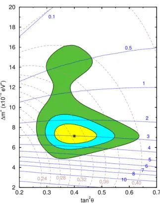
1). Precise measurements of the CC/NC ratio at SNO. In Fig. 6 we show the contours of constant CC/NC ratio. We find predictions for the best fit point and the3σinterval:
CC
NC = 0.33±0.08, 3σ. (24)
0.2 0.3 0.4 0.5 0.6 0.7 tan2θ
2 4 6 8 10 12 14 16 18 20
∆
m
2 (x10 −5 eV 2 )
0.1
1
2
3
4
5 6 7 8 10
0.24 0.28 0.32
0.36 0.40
0.5
Figure 6. Predictions for the CC/NC ratio and the Day-Night asym-metry at SNO. The dashed lines are the lines of constant CC/NC ratio (numbers at the curves) and the dotted lines show the lines of constantASN ODN (numbers at the curves in %). We show also the
(1σand3σ) allowed regions of the oscillation parameters from the combined fit of the solar neutrino data and the KamLAND spec-trum. The best fit point is indicated by a star.
Precise measurements of the ratio CC/NC will also strengthen the upper bounds on mixing and∆m2
.
2). The day-night asymmetry at SNO.The KamLAND pro-vides a strong lower bound on∆m2, and shifts the best fit point to larger∆m2. This further diminishes the expected value of day-night asymmetry. In Fig. 6 we show the con-tours of constant ASN O
DN . The best fit point prediction and
the3σbound equal
ASN ON D = 3.0±0.8%, (1σ), ASN ON D <6% (3σ). (25)
The present best fit value of the SNO asymmetry, 7%, is accepted at about 99% C.L.. The expected asymmetry at Super-Kamiokande is even smaller: In the best fit point we expectASK
N D ≈(1.7−2.0)%.
3). The turn up of the spectrum at SNO and Super-Kamiokande at low energies. Using results of [22] we pre-dict for the best fit point (16) an increase of ratio of the ob-served to expected (without oscillation) number of the CC events, RCC
SN O, from 0.31 at 8 MeV to 0.345 at 5 MeV, so
that RCC
SN O(5MeV)−RCCSN O(8MeV) RCC
SN O(8MeV)
= 0.10−0.12. (26)
In Super-Kamiokande the turn up is about(5−7)%in the same interval (5 - 8) MeV.
4). Further KamLAND measurements. Possible impact can be estimated using Figs. 1, 4. A decrease of the error by fac-tor of 2 (which will require both significant increase of sta-tistics and decrease of the systematic error) will allow Kam-LANDaloneto exclude all the regions but the l-region at 95 % C.L., if the best fit is at the same point as it is determined now.
5). BOREXINO.At3σwe predict the following suppressi-ons of signals with respect to the SSM predictisuppressi-ons to BO-REXINO experiment [23], in the two allowed regions:
RB(l−region) = 0.61−0.73,
RB(h−region) = 0.62−0.73. (27)
So, BOREXINO will perform consistency check but it will not distinguish the l- and h- regions.
6). Gallium production rate. In the best fit point one pre-dicts the germanium production rate QGe = 71 SNU. In
the h-region best fit pointQGe = 72SNU. So, the Gallium
experiments do not discriminate among the l - and h - regi-ons. However, precise measurements ofQGeare important
for improvements of the bound on the 1-2 mixing and its deviation from maximal value.
6
Conclusions
1. The first KamLAND results (rate and spectrum) are in a very good agreement with the predictions based on the LMA MSW solution of the solar neutrino problem.
2. Our analysis of the KamLAND data reproduces well the results of the collaboration. The oscillation parameters ex-tracted from the KamLAND data and from the solar neutrino data agree within1σ.
3. We have performed a combined analysis of the solar and KamLAND results. The main impact of the KamLAND re-sults on the LMA solution can be summarized in the fol-lowing way. KamLAND
• shifts the∆m2 to slightly higher values 6.3·10−5
→7.1·10−5eV2; (the mixing is practically unchan-ged: tan2θ = 0.40, and this number is rather stable with respect to variations of the analysis;
• establishes rather solid lower bound on the ∆m2 : ∆m2>4.8·10−5
eV2(3σ);
4. The KamLAND results strengthen the upper bound on the expected value of the day-night asymmetry at SNO: ASN O
DN <6%. We predict about 10% turn up of the energy
spectrum at SNO in the interval of energies (5 - 8) MeV. The CC/NC ratio is expected to be CC/NC≈0.33, that is, above the new SNO salt phase experimental result.
Future SNO measurements of the CC/NC ratio and ASN O
DN will have further strong impact on the LMA
para-meter space.
Aknowledgments
References
[1] K. Eguchiet al., KamLAND collaboration, Phys. Rev. Lett. 90, 021802 (2003).
[2] J. N. Bahcall, “Neutrino astrophysics”, Cambridge U. Press, Cambridge, England, 1989.
[3] B. T. Clevelandet al., Astroph. J.496(1998) 505; K. Lande
et al., inNeutrino 2000Sudbury, Canada 2000, Nucl. Phys. B (Proc. Suppl.)50(2001) 21. (Here and in ref. [5], [6], [7] we cite the latest publications of the collaboration in which the references to earlier works can be found.)
[4] K. S. Hirataet al., Phys. Rev. Lett.651297 (1990).
[5] J. N. Abdurashitov et al. (SAGE collaboration), J. Exp. Theor. Phys.95, 181 (2002); Zh. Eksp. Teor. Fiz.122, 211 (2002).
[6] T. Kirstenet al., Talk given at the 20th Int. Conf on Neutrino Physics and Astriphysics, Neutrino 2002, Munich, Germany, May 25 - 30, 2002.
[7] S. Fukuda et al. (Super-Kamiokande collaboration) Phys. Rev. Lett.86, 5651 (2001); Phys. Rev. Lett.86, 5656 (2001).
[8] Q. R. Ahmadet al., SNO collaboration, Phys. Rev. Lett.87, 071301 (2001).
[9] Q. R. Ahmadet al., SNO collaboration, Phys. Rev. Lett.89, 011301 (2002).
[10] Q. R. Ahmadet al., SNO collaboration, Phys. Rev. Lett.89, 011302 (2002).
[11] L. Wolfenstein, Phys. Rev. D17, 2369 (1978); S. P. Mikheyev and A. Yu. Smirnov, Yad. Fiz. 42, 1441 (1985) [ Sov. J. Nucl. Phys.42, 913 (1985)], Nuovo Cim. C9, 17 (1986); S. P. Mikheyev and A. Yu. Smirnov, ZHETF,91, (1986), [Sov. Phys. JETP,64, 4 (1986)].
[12] V. Barger, D. Marfatia, K. Whisnant, and B.P. Wood, Phys. Lett. B537, 179 (2002); A. Bandyopadhyay, S. Choubey, S. Goswami, and D. P. Roy, Phys. Lett. B540, 14 (2002); J. N. Bahcall, M.C. Gonzalez-Garcia, and C. Pe ˜na-Garay, JHEP 0207, 054 (2002); A. Strumia, C. Cattadori, N. Ferrari, and F. Vissani, Phys. Lett. B541, 327 (2002); P. Aliani, V. Anto-nelli, R. Ferrari, M. Picariello, and E. Torrente-Lujan, Phys. Rev. D67, 013006 (2003); G.L. Fogli, E. Lisi, A. Marrone, D. Montanino, and A. Palazzo, Phys. Rev. D66, 053010 (2002); M. Maltoni, T. Schwetz, M.A. Tortola, and J.W.F. Valle, Phys. Rev. D67, 013011 (2003). M. Smy, hep-ex/0208004.
[13] P. C. de Holanda, A. Yu. Smirnov, Phys. Rev. D66, 113005 (2002).
[14] Q. R. Ahmadet al., SNO collaboration, Phys. Rev. Lett.92, 181301 (2004).
[15] P. C. de Holanda, A. Yu. Smirnov, Astropart. Phys.21, 287 (2004).
[16] J. N. Bahcall, M.H. Pinsonneault, and S. Basu, Astrophys. J. 555, 990 (2001).
[17] P. C. de Holanda, A. Yu. Smirnov, JCAP0302, 001 (2003).
[18] L. E. Marcucciet al., Phys. Rev. C63, 015801 (2001); T.-S. Park et al., Phys. Rev. C67, 055206 (2003), and references therein.
[19] V. N. Gribov and B. Pontecorvo, Phys. Lett. B28, 493 (1969).
[20] J. N. Bahcall, M.C. Gonzalez-Garcia, C. Pe ˜na-Garay, hep-ph/0212147.
[21] M. C. Gonzalez-Garcia, C. Pe˜na-Garay, Y. Nir, and A. Yu. Smirnov, Phys. Rev. D63, 013007 (2001).
[22] P.I. Krastev, A.Yu. Smirnov, Phys. Rev. D65, 073022 (2002).