A Work Project presented as part of the requirements for the Award of a Master Degree in Finance from the NOVA – School of Business and Economics.
SAVINGS AND INFLATION
–
A PANEL THRESHOLD MODEL
APPROACH
Mariana Miguel dos Reis Ferreira #2482
A project carried out on the Master in Finance Program, under the supervision of: Professor Paulo M. M. Rodrigues
This research investigates the impact of inflation on savings through a panel of 42 countries observed annually between 1995 and 2014. A panel threshold model approach is followed, being one-year lagged inflation the threshold variable and gross savings the dependent one. Findings suggest that inflation has a positive impact on gross savings, particularly at lower levels of inflation. The robustness tests conducted led to conclude that the model does not hold for less developed economies where savings are not so correlated with the inflation level as it is among developed economies.
Keywords: savings, inflation, panel threshold mode
3 1. Introduction
Nine years have passed since the peak of the financial crisis that has impacted economies throughout the world. Indeed, the crisis has boosted inequalities, contributing to the shrinking of the middle class, while increasing poverty and consequently intensifying the accumulation of wealth in a smaller share of the society. Also, in the latest years, economic growth and social development have stand still as a consequence of a slow recovery process. Nevertheless, some emergent economies have arisen in recent decades, being however in early stages of development when compared to world’s major economies. Undoubtedly, the world is as heterogenous as diverse. Though progress has been generally witnessed everywhere, its growth rate is completely different, increasing disparities and boosting inequalities among countries. These differences are indeed very clear in terms of economic growth, investment, savings and debt.
As a mean for resource accumulation and to somehow finance economic growth, national savings are of extreme importance for national governments. If an increase in national savings allows for economic growth which allows for progress and development at a social level, this may be the key for progress – or is it a virtuous cycle and it is the economic growth that boosts savings, intensifying poverty traps of under-saving and sluggishness? The supposed stagnation or even decreasing trend of savings has become a central concern for economies. Inflation enters in the equation, considering the twisted effects that it intendedly has on economic growth when above a certain level. Thus, what should be the expected impact of inflation on savings? Which is the response of gross savings in scenarios of high and low inflation? For this matter, what is, objectively, high and low inflation?
4 Summing up, the findings led to one main conclusion: inflation has a positive impact on gross savings, particularly when it is at lower levels. This relation is, nonetheless, different across countries. The model does not hold for less developed economies, leading to the conclusion that there are other circumstances driving the level of savings in developing economies, rather than inflation.
This methodology adds to the literature providing that it allows to estimate the dynamic impact of inflation on savings, considering different correlations when the inflation is at its lower levels compared to higher levels. Furthermore, the use of an heterogenous sample of countries and the validation of the model for countries according to their development level avoids blind statements and strengthens the research conclusions. This study is organized as follows. Section two covers related literature on savings and inflation theories. Section three presents a conceptual framework and some statistical data. Section four describes the methodology followed and the model’s estimation. In section 5 results are discussed and finally section six sums up the work done, presenting concluding remarks.
2. Theoretical Framework
2.1. Origin of Savings
At a micro level, savings are perceived as future consumption, meaning that households delay present consumption to the future. At a macro level, e.g. a country scale, savings can be seen as a resource for long-term economic stability and prosperity. This last category, includes households’ personal savings and also government and corporate sector’s savings. In fact, according to the World Bank, gross savings correspond to the difference between disposable income and consumption.
5 utility levels – permanent-income hypothesis (Friedman, 1957). In this way, consumption in a certain moment is not determined by income in that exact moment but by aggregate income over the individual’s entire lifetime. Therefore, by saving, individuals are splitting their current income between current and probable future needs, letting themselves the possibility of satisfying consumption needs later. The second main reason for saving relies on Carroll & Summers (1991) and Carroll’s (1996) research and is related with precautionary motives, i.e., people save to have a provision against eventual unexpected needs. Finally, savings may be generated due to the perception that households have of investment opportunities, as in, high interest rate and high income return.
More recently, the intention to leave a bequest has also been pointed out has a motivation to save, particularly in older ages, though the excess savings as a consequence of this fact seems narrow (Carroll, 2000). Indeed, (Beckmann, Hake, & Urvova, 2013) have empirically1 found that the dissaving behaviour at older ages predicted by the life-cycle
hypothesis is not that significant, relating that with an eventual bequest motive or even with the memory of past economic turbulence.
Ideally the abovementioned reasons to save could apply to everyone, and consequently every country. However, considering the disparities in savings’ distribution across countries, it seems that there is more on the root of savings rather than a smoothing of the consumption path. More than assessing why some agents save and why others do not, it is also the object of this study to perceive the consequences of both of these behaviours, i.e., why do savings matter.
2.2. Savings as a mean to boost economic growth
Solow (1956) introduces the saving rate as part of output that is left from consumption and is allocated to investment. Accordingly, the Solow Growth Model, states that from the income received, the portion that is not consumed is the source of investment. Thus, an increase in investment leads to economic growth, since growing environments boost investment opportunities. In this sense, the Solow model supports a positive relation between savings and economic growth. However, it matters to highlight that this relation does not hold indefinitely in the long-run, i.e., there is no continuous growth. The boost in economic growth caused by the increase in capital stock is temporary, holding only
1 Analysis on households’ saving behavior in Central, Eastern and Southeastern European countries
6 until the moment in which the economy reaches the new steady-state level of output – as in, the long-run equilibrium of the economy.
Among others, also Harrod (1939) and Domar (1946) found evidence of a positive link between savings and economic growth reached through investment. Deaton (1977) reached a similar conclusion, stressing, however, the question of knowing if it is savings that are in the root of economic growth, or if it is economic growth behind the higher savings rate or even if it is both hypotheses, simultaneously.
Several long-run growth theories, such as the “AK” theory (Romer, 1986), raise however a different approach, according to which savings lead to permanent rather temporary economic growth. This theory is supported by the fact that savings, as accumulation of capital, may be transferred to intellectual capital that allows for technological progress implying a faster growth for these economies than investing in human and physical capital.
Following the same line of thought, Aghion, Comin, Howitt, & Tecu (2009) have empirically concluded that savings are indeed central for the adoption of technology particularly in developing economies. Accordingly, developed economies have at its disposal the latest technological equipments to boost their businesses, production and economic growth. However, developing countries face higher costs to employ technology, relying on either foreign investors or their own capital previously accumulated.
Contrarily to the above mentioned positive links, the paradox of thrift of John Maynard Keynes predicts that households’ saving may impact negatively on the economy at a country level by the simple idea that while saving, households are not consuming as much as they could, therefore harming corporates’ earnings. Ultimately, this effect would mean a rise in unemployment rates, leading to a decrease in savings after all. The counter-argument to this theory relies on the increased liquidity that personal savings allow banks to have, i.e., with an increase in households’ savings, banks have a higher buffer of money to concede loans to finance companies’ investments.
2.3. Savings’ distribution across developed and less developed economies
7 a virtuous cycle of savings-growth. This would imply that developed economies are in a favourable situation where prosperity boosts savings and vice-versa. Yet, for less developed economies the scenario is much more adverse: proving to be true, how is it possible for these countries to leave the poverty trap in which they are stuck?
Loayza, Schmidt-Hebbel, & Servén (2000a) investigated savings in developing economies, pointing market imperfections and policy distortions as a cause for a low level of national savings. Also Deaton (1989) supported that research on savings’ topics should make a clear distinction between the development state of the countries considered. Accordingly, from a micro perspective, Deaton considers that households in less developed economies tend to be larger (highly populated countries) and poorer, with uncertain income and rural jobs, not being reasonable to assume a model of income allocation over time. Indeed, Deaton finds that the tendency for several generations to live together and ultimately the stationarity demographic structure, under which the oldest dies and is replaced by a new-born, eliminates the typical lifecycle under which there is a retirement period and there is a need to save for that period – to smooth consumption. In this case, it is considered that resources are shared among the generations between dependents and workers. From a macro point of view, few developing economies have a fiscal system that allows for “manipulation of personal disposable income to help stabilize output and employment”(Deaton, 1989: 62). Additionally, Deaton (1989) points the lack of government policies and the low reliability of accurate data on savings as additional constraints in the analysis of savings in developing countries.
8 for individuals’ current well-being and survival. Therefore, especially in developing countries, where income is typically lower and with a high uncertainty, these expenditures cannot be postponed to smooth consumption. Obviously, this approach is not applicable in developed economies where this type of consumption is so basic that it is not questioned.
Despite the above mentioned ideas seemed to prevent the motivations to save in less developed economies, Gersovitz (1988) has also stated that savings are an intertemporal process due to its ability to produce additional output for future consumption, hence being vital for the development of poorer economies. Together with the fact that foreign capital investments in developing economies may increase “threats of expropriation, repudiation and other hostile acts against foreign suppliers of capital” (Gersovitz, 1988: 382), the author still considers national savings the main source of capital accumulation even in developing economies.
Though savings and investments are not exclusive conditions for the development and growth, literature shows that they surely work as a vital engine, enhancing and strengthening the country’s macroeconomic environment in the long-term. Indeed, the differences between developed and less developed countries at an economic and social level are so deep that different approaches are required, since the determinants of savings in highly developed countries – which are nowadays generally known and measurable – are different from those in developing ones. Therefore, the question for further research is: what determines savings in developing economies and how can it increase?
2.4.How does inflation impact savings?
“Inflationis always and everywhere a monetary phenomenon in the sense that it is and can be produced only by a more rapid increase in the quantity of money than in output”
(Friedman, 1970) Understanding inflation implies understanding what are its causes, i.e., which factors are behind the increase in the general level of prices. Due to its importance in economies through the impact that it has on economic growth, by distorting or fostering it – no consensus has been reached yet among the economic community – inflation has been a matter of study for decades.
9 of them providing a unique and conclusive answer. Furthermore, a few authors are in support of a no-impact theory, in the long run, provided that money is super-neutral2 in
the steady state, therefore considering an elastic labour supply, the savings rate may increase or decrease with inflation (Heer & Sussmuth, 2009; Sidrauski, 1967). Haque, Pesaran, & Sharma (1999) have equally concluded about no empirical long term influence of inflation on private savings in a panel of OECD countries.
Also, some authors make a distinct analysis between anticipated inflation and unanticipated inflation, stating that the impacts might be different considering that, in the former the increase in prices is known in advance, thus economic agents can handle it properly, leading to a null impact on economic behaviour (Thomas Juster & Wacthel, 1972); while the consequences generated by the latter and the uncertainty associated may impact considerably more on the economy.
There are two main theories in favour of a positive correlation between savings and inflation. Firstly, according to Deaton (1977) whose aggregate demand model considers that in the presence of unanticipated inflation, economic agents may not perceive the increase in prices as inflation, considering that consumers do not hold enough information to make that distinction i.e., instead of recognizing an increase in general price levels, households may perceive only an increase in some prices. Consequently, consumption may decrease in the sense that agents will search for substitute commodities later. Therefore, unanticipated inflation impacts positively on the savings rate (Davidson & MacKinnon, 1983). Secondly, the higher the rate of inflation, the higher is the percentage of income that is not actually income but a mere compensation for the generalized decrease in the real value of money. Hence, also interest income is inflated and it is not entirely real income, implying that in order to keep the real value of wealth, the proportion of savings has to increase providing that dividend income cannot be used to finance consumption (Davidson & MacKinnon, 1983).
Thomas Juster & Wacthel (1972) have also conducted an empirical study on the impact of inflation on the ratio of personal savings to personal income and concluded that anticipated inflation has a small positive effect on savings while unanticipated inflation has a larger positive impact. These findings support the theory suggested by the same authors that with inflation, the variance of expected real income induces asymmetrical effects on consumers’ behaviour. Indeed, the consequences of spending in a scenario
10 where future real income3 has not grown as much as expected, are much worse than the consequences of not spending – as in, saving – in a scenario where future real income as increased more than expected.
Empirical studies from Loayza, Schmidt-Hebbel, & Servén (2000b) conclude also in favour of a positive relation between inflation and private savings. In their work, the authors have used inflation as a proxy for uncertainty. Hence, the positive correlation found is justified by the precautionary reason to save that economic agents perceive. Nevertheless, Loayza et al. (2000b) highlight that the contrary effect is not linear, i.e., inflation’s stabilization may not imply a proportionate decrease in savings, considering that with steady inflation levels savings are positively impacted (indirectly, e.g.: via economic growth) which offsets the negative effect.
Contrarily to the ideas presented above, some authors in recent decades, have found a negative link between inflation and savings. Feldstein (1982) approached the relation between these two variables through the tax burden on capital income. Accordingly, the author concluded that once inflation fictionally increases returns on savings, the taxable amount is higher, leading to a higher tax rate on income. In this way, taxation is not proportional to the real income that economic agents receive, which gets particular relevance for small savers, who are penalized instead of rewarded. Heer & Suessmuth (2005) have also corroborated this theory, through an overlapping generations model, concluding in favour of a decrease in savings after an increase in inflation, associated with higher taxation of interest income. However, there is also the contrary effect, i.e., as interest income is typically computed in nominal terms, a higher inflation rate can be perceived as an incentive to save more providing the capital gain will be higher (though not 100% real).
Taking all of this into consideration, the model presented in the following sections attempts to assess to what extent inflation affects savings and which other external factors are weighting in this relation, estimating a threshold value for inflation above which this relation might change.
3 The increase in real income occurs because the growth rate of money income is higher than the growth
11 3. Conceptual Framework
3.1. An overview of savings’ distribution in the world
In the end of 2015, gross financial assets around the world amounted circa (c.) 155 trillion euros within bank deposits, securities and insurance, and pension funds4. Theoretically, this amount would more than pay off all the world’s sovereign debt (c. 52 trillion euros). A blinded overview of these numbers would be perceived as a positive sign of equal economic growth and prosperity. The problem is that throughout the history there has always been inequalities. Enough to say that this numbers result from an analysis of 53 countries (over 192 belonging to the United Nations) that represent 90% of the world’s GDP and 69% of world’s population. From here, one may infer an obvious conclusion: if 90% of global GDP respects to only 69% of global population, the remaining 31% are substantially poorer.
Countries are now in different stages of economic and human development, meaning that economic indicators, in which savings are included, vary widely. Having in mind the consensual positive correlation between savings and economic growth, it is straightforward that more developed regions present higher savings values. Indeed, differences begin at a more micro level, between individuals in a same region or country, evidencing a close relation between income and savings. Nonetheless, the inherent idea that poor people save less is contrary to the lifecycle hypothesis providing that lower-income agents should have low lower-income perspectives for the future too, therefore they would need to save proportionally the same as wealthier do, to smooth consumption. Indeed, according to a World Bank report5, in the late 60s, the rate of savings in low-income economies was around 13% of its low-income while in high-low-income economies it was c. 21%. However, there was a shift in this trend: in 2009, the rate of savings of developing economies rose to 32% of its income, compared to a decrease in developed economies’ savings to 17%. This change was associated mainly with ageing populations, economic growth and deepening of financial markets5. These are also the factors that are projected to continue determining the variations in savings’ rate, however in some regions, the negative impact of ageing may be offset by the positive impact of economic growth leading to a stabilization of savings (as for example, Indonesia)5.
4 Brandmeir, Grimm, Heise, & Holzhausen (2016) considering 53 countries, representing c. 90% of world’s GDP and 69% of world’s population.
12 Though the savings rate in developing economies seems to be concentrated in high-income households, World Bank projects a convergence trend between developed economies and a large group of developing countries in terms of income, consequently projecting an increase in growth rates and thus in savings.
Analysing figure 1, it is possible to conclude that Asia appears in the top regions with higher gross savings in percentage of GDP, corroborating the idea presented above that developing economies are facing an increase in savings rate. In fact, even South Asia has registered a significant increase in its savings with a peak in 2007. Contrarily, Europe & Central Asia, as well as North America – perceived as more homogeneous regions in terms of development – present a stable pattern of savings, averaging 22,5% and 19,13% of GDP,
respectively, between 1980 and 2015. China is commonly accepted as the main contributor to the boost in savings rate in Asia, because of its exponential growth over the past decades.
Additionally, the low savings percentage of Sub-Saharan Africa – the lowest among the regions considered – is justified partially due to its development state that is significantly behind other developing regions, presenting also a slower growth rate.
Figure 2 presents the three countries with higher and lower average gross savings in percentage of GDP, among the countries considered in the model developed in the following section. Indeed, the top 3 countries are in fact less developed economies according to the United Nations’ classification. Among the 3 with lowest rates, only the United Kingdom is considered a developed economy. Concluding, among the developing
5 15 25 35 45 55
1980 1985 1990 1995 2000 2005 2010 2015
Figure 1: Gross Rate of Savings in percentage of GDP between 1980 and 2015.
Source: World Bank Database and authors’
calculation 5 15 25 35 45 55 65
Figure 2: Gross Rate of Savings in percentage of GDP between 1995 and 2013 among some countries of the sample considered in the empirical model. Source: World Bank Database
13 economies the disparity of development levels is very wide leading to completely opposite records in terms of savings too.
3.2. A comparative analysis – savings and inflation behaviour
A comparative analysis on historical data of inflation (annual percentages) and gross savings (in percentage of GDP), presented in figure 3 below, show some similar movements, as for instance a peak in 2007-2008 and a downturn in 2009. However, there are also some disparities in the variations observed, as in the more recent years, in which savings seem to increase or stabilize while inflation seems to be decreasing.
By observing past data, it is not possible to take one straight conclusion of the correlation between the two variables, mainly because several exogenous factors that are not being considered here, can bias the conclusions. Nevertheless, this plot enabled us to assess the evolution that these two variables have been registering over the years, from where we conclude that – despite the fluctuations – the initial and ending period results reveal that savings are quite constant, whereas inflation has whiteness a significant decrease, being on average closer to zero now.
Figure 3: Comparison between the gross rate of savings in percentage of GDP and inflation in annual
percentage. Source: World Bank Database and authors’ calculation
4. Empirical Analysis of the Model
The aim of this study is to apply a dynamic panel threshold model to investigate the impact of inflation on gross savings in developed and less developed economies. To do so, annual data from 42 countries (detailed in Appendix A) between 1995 and 2014 gathered from World Bank Database was used. The range of countries in this study encompasses 20 developed and 22 less developed economies, selected according to the
-5 0 5 10 15 20 25 30 35 40
1980 1985 1990 1995 2000 2005 2010
Savings OECD
Savings World
Inflation OECD
Inflation World
Savings Average (sample 42 countries)
14 United Nations classification available in the World Economic Situation Prospects (United Nations, 2016) and considering mainly the ones with higher GDP and Population. Following Kremer, Bick, & Nautz (2013) this study is conducted by extending Hansen’s approach (Hansen, 1999) to consider endogenous regressors. Indeed, this was the main factor considered in the choice of this methodology, since it is crucial to include the one year lagged gross savings as explanatory variable even though it brings endogeneity, considering the implicit impact that it has on gross savings at t=0. In this sense, this model allows for endogeneity considering the use of generalized methods of moments (GMM) estimation following Caner & Hansen (2004).
In this model, the role of inflation’s thresholds is assessed in the relation between inflation and gross savings, where the threshold variable is the initial inflation (iit-1)and gross
savings is the dependent variable (yit = Sit). The endogenous regressor will be the one year
lag of gross savings (Sit-1). Several control variables are also included to account for
exogenous regime-independent factors that may impact gross savings. Its choice was based on the literature and its expected impacts are further detailed in the section 4.2. The construction of this model proceeded in two phases, as detailed in the following section. In the first phase, a linear equation that assesses the determinants of savings was defined. In the second phase the threshold effect was introduced, where two equations are estimated which consider the behavior of savings for low and high levels of inflation. Finally, a robustness check is conducted, to assess the validity of the estimated model in the two sub-groups of developed and less developed economies, concluding to what extent the results vary according to the country’s development state.
4.1.The model
4.1.1. The linear equation model
According to the literature presented in section 2, the empirical model used in the first step
can be translated in the following linear equation:
𝑆𝑖,𝑡 = 𝜇𝑖+ 𝛽1𝑆𝑖,𝑡−1+ 𝛽2𝐺𝑁𝐼𝑖,𝑡 + 𝛽3𝑅𝑖,𝑡 + 𝛽4𝑈𝑖,𝑡 + 𝛽5𝐿𝑖,𝑡 + 𝛽6𝐸𝑖,𝑡 + 𝜀𝑖𝑡 (1)
where: 𝒊 = 1, 2, … , 42 𝑑𝑒𝑛𝑜𝑡𝑒𝑠 𝑐𝑜𝑢𝑛𝑡𝑟𝑖𝑒𝑠 and 𝒕 = 1, 2, … , 20 𝑑𝑒𝑛𝑜𝑡𝑒𝑠 𝑦𝑒𝑎𝑟𝑠.
15
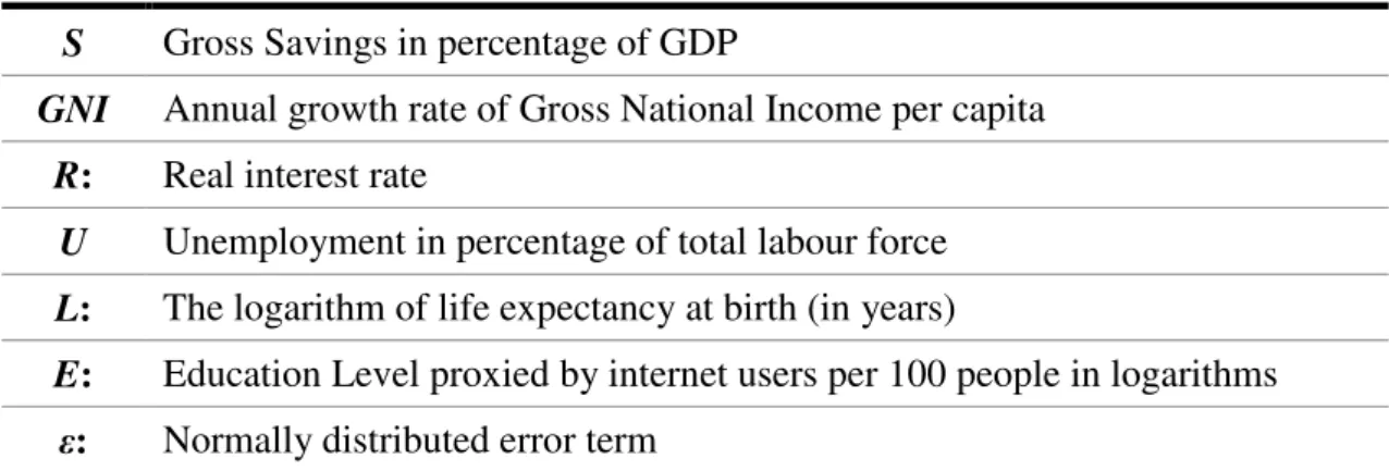
S Gross Savings in percentage of GDP
GNI Annual growth rate of Gross National Income per capita
R: Real interest rate
U Unemployment in percentage of total labour force
L: The logarithm of life expectancy at birth (in years)
E: Education Level proxied by internet users per 100 people in logarithms
ε: Normally distributed error term
Table 1: Variables’ definition
More information on the definition of each variable can be found in appendix B. Model estimations were performed using Stata 13 and Matlab 2017.
In the equation defined above, 𝜇𝑖 stands for country specific fixed effects that despite unobservable, may impact the dependent variable, being determined by country’s cultural or geographical characteristics. According to Hausman (1979), these effects may be either (i) random, i.e., not correlated with explanatory variables or (ii) fixed, if the individual effects are correlated with the explanatory variables and influencing the predicted output. In this way, the Hausman Test is conducted to assess the adequate way to treat country effects in this model. The null hypothesis is that both methods produce consistent estimators (𝐻0: 𝑐𝑜𝑒𝑓(𝑓𝑒) − 𝑐𝑜𝑒𝑓(𝑟𝑒) = 0) against the alternative hypothesis of only fixed effects producing consistent estimators (𝐻1: 𝑐𝑜𝑒𝑓(𝑓𝑒) − 𝑐𝑜𝑒𝑓(𝑟𝑒) ≠ 0). Results obtained (H = 216.49; p-value = 0), point to the rejection of the null hypothesis, implying that fixed effects are most appropriate in this case.
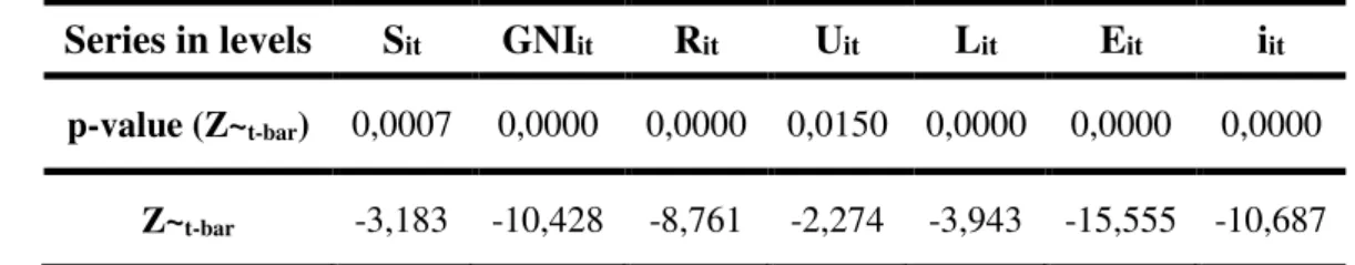
Prior to the introduction of the threshold variable, unit root tests were performed to assess if the data is stationary or non-stationary. Following Neal (2013) and despite the several test statistics that can be used to compute unit root tests, the authors have chosen the Im Pesaran and Shin (IPS) test considering that it is intended to be more powerful according to Monte-Carlo results obtained under the assumption of no cross-sectional correlation in panels (Im, Pesaran, & Shin, 2003).
16 Series in levels Sit GNIit Rit Uit Lit Eit iit
p-value (Z~t-bar) 0,0007 0,0000 0,0000 0,0150 0,0000 0,0000 0,0000
Z~t-bar -3,183 -10,428 -8,761 -2,274 -3,943 -15,555 -10,687
Table 2: Panel unit root test
The results presented confirm that for all variables except unemployment, the null hypothesis is rejected at a 1% significance level, meaning that with the exception of unemployment, all variables are stationary. As for unemployment, the null hypothesis is also rejected but in this case at a 5% significance level.
Although not included in the linear equation (1), inflation (iit) was also tested for unit
roots, as it is going to be introduced in the following phase of the methodology as the threshold variable. The results point also to the rejection of null hypothesis at a 1% significance level, indicating the stationary behavior of this variable.
4.1.2. The threshold model
Considering inflation as a threshold variable, the following panel threshold model is obtained:
𝑆𝑖,𝑡 = 𝜇𝑖+ 𝛼0𝐼(𝑖𝑖,𝑡−1≤ 𝛾) + 𝛼1𝑖𝑖,𝑡−1𝐼(𝑖𝑖,𝑡−1≤ 𝛾) + 𝛼2𝑖𝑖,𝑡−1(1 − 𝐼(𝑖𝑖,𝑡−1≤ 𝛾)) +
𝛽1𝑆𝑖,𝑡−1+ 𝛽2𝐺𝑁𝐼𝑖,𝑡 + 𝛽3𝑅𝑖,𝑡 + 𝛽4𝑈𝑖,𝑡 + 𝛽5𝐿𝑖,𝑡 + 𝛽6𝐸𝑖,𝑡 + 𝜀𝑖𝑡 (2)
As one can see from equation (2), one-year lagged inflation is both the threshold variable and the regime-dependent regressor, similarly to Kremer et al.'s (2013) methodology.
𝐼(𝑖𝑖,𝑡−1 ≤ 𝛾) is an indicator variable that assumes a value of 1 if inflation is below or equal
17 4.1.3. Estimation
Panel threshold models’ estimation starts with accounting for fixed effects (𝜇𝑖), as proposed by Kremer et al. (2013) . Accordingly, a forward orthogonal deviation transformation that “subtracts the average of all future available observations of a variable”Kremer (2013) is applied, avoiding correlation of the transformed error term that occurs in other fixed effects transformation’s methodologies, as referred by the abovementioned authors.
Thereafter, a procedure to treat eventual endogeneity constraints – arising from the possible correlation of the endogenous variables with the error term – is conducted. Following Baum, Checherita-Westphal, & Rother (2012) and Kremer et al. (2013) a two-stage least squares method (2SLS) is performed by estimating the reduced form of 𝑆𝑖,𝑡−1 , as a function of the above-mentioned instruments (𝑆𝑖,𝑡−2, 𝑆𝑖,𝑡−3, 𝑆𝑖,𝑡−4 and 𝑆𝑖,𝑡−5). The predicted values of this endogenous variable, 𝑆̂𝑖,𝑡−1 replace the original values (𝑆𝑖,𝑡−1) in the structural equation (2).
Then, the threshold value – 𝛾 – is estimated following Hansen (1999) by estimating equation (2) via 2SLS for each value of the threshold series, being the sum of squared residuals 𝑆𝑗(𝛾) kept. The threshold is then selected as the one that minimises the sum of squared residuals, i.e.: 𝛾̂ = 𝑎𝑟𝑔𝑚𝑖𝑛 𝑆𝑗(𝛾).
The critical values to determine the confidence interval of the threshold were computed according to Kremer et al. (2013), based on the asymptotic distribution of the likelihood ratio statistic LR (𝛾).
Having estimated the threshold –𝛾̂–, the slope coefficients of equation (2) are estimated by the generalized method of moments (GMM) for 𝛾̂ and the set of instruments previously used, as suggested by Baum et al. (2012).
4.2. Results
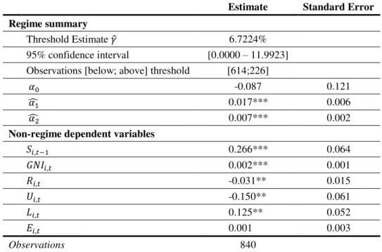
18 the correlation is higher when inflation is lower ( 𝛼̂ = 0.017)1 while for high levels of
inflation – above 6.7224% - the positive impact of inflation in gross savings is much lower ( 𝛼2̂ = 0.007).
Estimate Standard Error
Regime summary
Threshold Estimate 𝛾̂ 6.7224%
95% confidence interval [0.0000 – 11.9923] Observations [below; above] threshold [614;226]
𝛼0 -0.087 0.121
𝛼̂1 0.017*** 0.006
𝛼2̂ 0.007*** 0.002
Non-regime dependent variables
𝑆𝑖,𝑡−1 0.266*** 0.064
𝐺𝑁𝐼𝑖,𝑡 0.002*** 0.001
𝑅𝑖,𝑡 -0.031** 0.015
𝑈𝑖,𝑡 -0.150** 0.061
𝐿𝑖,𝑡 0.125** 0.052
𝐸𝑖,𝑡 0.001 0.003
Observations 840
Table 3: Inflation thresholds and savings.
Notes: ***/**/* indicate significance at 10%, 5% and 1% level, respectively.
According to the experimental run with one instrument only (Appendix C), it is possible to conclude that the model presented above is robust also in the instruments chosen, considering that an experimental run with only one instrument does not produce significant changes in the outputs, not even in the confidence intervals – that remained almost unchanged.
As for the non-regime dependent variables, introduced to control for exogenous impacts on gross savings that are nonetheless considered relevant to explain gross savings’ variations, one can see from table 4 that all, with the exception of education level, are statically significant in the model. The coefficients’ sign of these variables are the expected according to literature, meaning that the level of savings from the previous period, the gross national income and the life expectancy in years are perceived to have a positive impact on the dependent variable. Contrarily, the real interest rate and unemployment seem to have a negative influence on gross savings.
19 increases and the level of consumption remains steady, savings might increase. As for real interest rate, the estimated impact is negative similarly to the results found by Loayza et al. (2000b). Though the rate considered is not exactly a rate that translates the dividend income for any financial asset, having in mind the substitution effect, it is reasonable to assume a negative correlation between savings and interest rates. Accordingly, as savings are future consumption, consumers would be willing to postpone consumption if they are adequately compensated. In a scenario of low interest rates, there is no incentive to postpone consumption which increases current consumption, thus decreasing savings (El Mekkaoui de Freitas & Oliveira Martins, 2014).
Unemployment impacts negatively savings based on the natural understanding that unemployed agents will use accumulated savings to compensate the loss in current income, meaning that they dissave (Dynarski, Gruber, Moffitt, & Burtless, 1997). Finally, the positive correlation found between life expectancy and the dependent variable may be a consequence of the increase in savings at older ages – that contributes to the increase in general savings – since the weight of elderly people increases with the increase in life expectancy. El Mekkaoui de Freitas & Oliveira Martins (2014) and Bloom, Canning, & Graham (2003) have reached the same conclusions.
4.3. Robustness Check
20
Developed Economies Less Developed Economies
Regime summary Period: 1995 – 2014 Period: 1995 – 2014 Period: 2003 – 2014
Threshold Estimate 𝛾̂ 4.2199% 6.7653% 4.863%
95% confidence interval [3.0069 – 7.3610] [0.0000 – 13.8811] [0.0000 – 10.9076] Observations [below; above]
threshold [309;91] [266;174] [123;141]
Estimate Standar
d Error Estimate
Standard
Error Estimate
Standard Error
𝛼0 -0.157 0.157 0.015 0.166 0.079 0.428
𝛼1 0.016** 0.006 0.012 0.09 -0.019 0.020
𝛼2 0.005*** 0.002 -0.036 0.031 -0.081 0.092
Non-regime dependent variables
𝑆𝑖,𝑡−1 0.253*** 0.063 0.292*** 0.087 0.208** 0.098
𝐺𝑁𝐼𝑖,𝑡 0.002*** 0.001 0.002*** 0.001 0.003** 0.001
𝑅𝑖,𝑡 -0.039** 0.019 -0.008 0.024 0.034 0.044
𝑈𝑖,𝑡 -0.076 0.078 -0.198** 0.078 0.382 0.215
𝐿𝑖,𝑡 0.435*** 0.088 0.061 0.064 -0.381 0.209
𝐸𝑖,𝑡 -0.009*** 0.002 0.002 0.002 0.004 0.008
Observations 400 440 264
Table 4: Inflation thresholds and savings – comparison between developed and less developed economies Notes: ***/**/* indicate significance at 10%, 5% and 1% level, respectively.
4.3.1. The impact of inflation on savings in developed economies
Results for developed economies are detailed in the first column of table 4, based on 400 observations from 20 countries. The threshold estimate – 𝛾̂ = 4.2199% – is significantly
lower than the one obtained in the aggregate model. The 95% confidence interval has considerably shorten being now between 3.0069% and 7.3610%.
The model’s output in developed economies is identical to the aggregate model, pointing to a positive impact of inflation on gross savings that is more significant in lower levels of inflation rather than in high inflationary state. These results are as well in accordance with theory.
21 investigated the influence of education on income, in the sense that higher educated agents tend to have an higher income which allows them to have a higher savings’ rate. Furthermore, higher educated profiles will naturally be more future-oriented which impacts their consumption behaviour. Finally, higher levels of education relate with increased financial literacy, typically leading to better and sound investments, relying on less debt (Yamokoski & Keister, 2006). Nevertheless, some authors, including Solmon (1975) consider an eventual negative relation between these two variables. Indeed, the increase in income boosted by a solid educational background provides financial stability, diminishing the reasons to hold precautionary savings and increasing consumption. In developed economies, it seems reasonable to assume this behaviour from economic agents, justifying the negative coefficient estimated (-0.009).
4.3.2. The impact of inflation on savings in less developed economies
The second column of table 4 presents the results of the model adjusted for the sample of less developed economies. It considers 440 observations from 22 countries. These results differ substantially from the developed economies’ model. Starting with the threshold estimate – 𝛾̂ = 6.7653%–which is higher than in the previous two models. As for the confidence interval, it has widened, ranging now from 0 to 13.8811% which indicates that estimation might be less efficient.
22 regimes has become more balanced than in developing economies – with 123 observations below the threshold and 141 observations above it – meaning that the inflation sample itself is more heterogenous or else, most observations would be above (below) the threshold and just a few below (above).
Due to the non-significance of the threshold model, a linear fixed effects regression was estimated, following the above equation.
𝑆𝑖,𝑡 = 𝛼𝑖+ 𝛽1𝑖𝑖,𝑡−1+ 𝛽2𝑆𝑖,𝑡−1+ 𝛽3𝐺𝑁𝐼𝑖,𝑡 + 𝛽4𝑅𝑖,𝑡 + 𝛽5𝑈𝑖,𝑡 + 𝛽6𝐿𝑖,𝑡 + 𝛽7𝐸𝑖,𝑡 + 𝜀𝑖𝑡 (3)
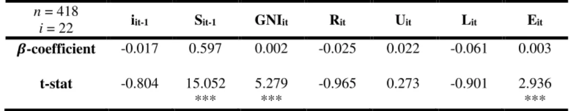
Results presented in table 5 point to the non-significance of the inflation levels to determine gross savings. Contrarily, one-year lag of savings appears to be determinant in the gross savings values of the current period, having a very high positive coefficient associated (𝑆̂𝑖,𝑡−1 = 0.597). Also, the gross national income and education level contribute positively to the variations in gross savings. From the opposite sign of the education’s coefficient – that is positive in less developed countries and negative in developed countries – one may conclude that indeed for developed economies higher educated households have higher financial stability and may disregard a precautionary savings behaviour (Solmon, 1975). However, this is not the case for developing economies, in which the positive coefficient may be the reflection of a higher income boosted by more educated profiles with future orientation and increased financial literacy.
n = 418
i = 22 iit-1 Sit-1 GNIit Rit Uit Lit Eit
𝜷-coefficient -0.017 0.597 0.002 -0.025 0.022 -0.061 0.003
t-stat -0.804 15.052
***
5.279 ***
-0.965 0.273 -0.901 2.936 ***
Table 5: Fixed effects estimation for less developed economies (time frame: 1995-2014)
Notes: the null hypothesis is that 𝑯𝟎: 𝜷𝒊= 𝟎. Notes: ***/**/* indicate significance at 10%, 5% and 1% level, respectively.
23
n = 308
i = 22 iit-1 Sit-1 GNIit Rit Uit Lit Eit
𝜷-coefficient 0.013 0.481 0.003 -0.003 0.141 -0.260 0.011
t-stat 0.255 9.792
***
5.867 ***
-0.089 1.432 -2.309 **
3.506 ***
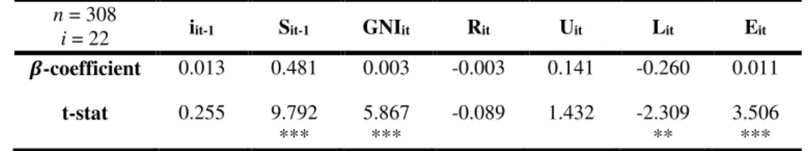
Table 6: Fixed effects estimation for less developed economies (time frame: 2003-2014)
Notes: the null hypothesis is that 𝑯𝟎: 𝜷𝒊= 𝟎. Notes: ***/**/* indicate significance at 10%, 5% and 1% level, respectively.
Despite inflation remaining not significant, the model has become more robust in what concerns to explanatory variables, being the life expectancy also a significant variable to explain savings’ variation. In fact, the negative contribution of life expectancy for savings supports the life-cycle theory according to which savings are intended to serve future consumption, which is not applicable to elderly because they are in the second period of the life-cycle (retirement) in which they consume, i.e., dissave. Following this, an increase in life expectancy followed by an increase in ageing population would mean a decrease in savings. Furthermore, it is important to highlight the strength of the fixed effects, meaning that the individual characteristics of each country seem to be quite critical in developing countries.
5. Discussion of Results
The model developed in the previous section supports the existing literature that inflation has a positive impact on savings. The threshold value estimated of 6.72% is the breakpoint above which inflation’s coefficient is lower, implying that, while still contributing positively to savings, in high inflation scenarios the impact is lower. The ideas presented by Deaton (1977), Davidson & MacKinnon (1983) and Thomas Juster & Wacthel (1972) are then corroborated. The inflation threshold estimated is quite high compared to the current inflation levels that central banks have been targeting – consider for instance the European Central Bank that has targeted an inflation rate below 2% for the Euro area – and the actual values observed lately – the average inflation rate in the sample of 42 countries on 2014 was 4.29%. Still, it must be taken into account that the countries’ sample considered is quite diverse.
24 main difference compared to the full model is the threshold value – that is substantially lower – which is in line with the inflation rates typically observed in more developed economies. Also in this sub-model, the impact of inflation above the threshold is much lower, which may announce that as inflation increases the impact it has on savings will tend to be zero – resembling the theory suggested by Sidrauski (1967) of a null impact in the long run savings.
Concerning less developed economies, results suggest that inflation is not statistically significant to explain gross savings. More specifically, gross savings does not even vary according to the level of inflation, not being reasonable to use a panel threshold for savings-inflation relation. In this way, for developeding countries, savings are linearly explained by income (GNI), unemployment and savings from the previous period rather than inflation. Similarly to Haque et al. (1999), who found no empirical statistically significance of inflation on private savings for a panel of OECD countries, these results point to an analogous conclusion but, in this case, for gross savings. Despite all the above mentioned, it is not straightforward why inflation has no significant impact on savings in developing economies. From a broader approach, it would be reasonable to assume that it should impact even if, indirectly, through economic growth.
Results obtained are very much aligned with the theory reviewed: either inflation has a positive impact on savings or no impact at all, positing as unlikely the negative contribution found by Feldstein (1982) in the theory of capital taxation.
6. Concluding Remarks
In this empirical analysis, the impact of inflation on national gross savings was assessed in a panel of 42 countries observed between 1995 and 2014. From the analysis performed it was possible to conclude that there is a positive link between inflation and savings, being more significant at lower levels of inflation. In this sense, savings tend to increase more with inflation when it is below 6.7% – the estimated threshold value above which the inflation impact on savings is quite reduced.
25 hold for developing economies in which gross savings vary in response to several other exogenous determinants, regardless of the inflation levels.
The explanatory variables’ significance, as well as its strength, varies between the full model and the two development level’s models, implying that if savings’ determinants are different depending on the development level of the country, the ways to boost it should also be different. Consequently, government policies should be defined accordingly.
The main limitation of this analysis is related to the time span considered – 20 years – that does not comprehend a sound period in which significant variations in the inflation values could be observed, particularly in developed economies. Indeed, for half of the countries considered, the difference between the maximum and minimum values observed is below 10%. Equally relevant is the methodological restriction of estimating only one threshold value. Considering the low positive impact that high inflation has on savings, one should not disregard the possibility of a negative impact of a super high inflation level.
The period under analysis encompasses another limitation to this research, given that it comprehends the period of the global economic and financial crisis – which has started in 2007 and has had repercussions along the following decade. Results may be biased due to some external shocks occurred as a crisis’ collateral effect and not exactly from any other endogenous matters.
26 7. References
Aghion, P., Comin, D., Howitt, P., & Tecu, I. 2009. When does domestic saving matter for economic growth? no. 09–080. https://doi.org/10.2139/ssrn.1328359.
Ando, A., & Modigliani, F. 1963. The“ life cycle” hypothesis of saving: Aggregate implications and tests. The American Economic Review, 53: 55–84.
Arellano, M., & Bover, O. 1995. Another Look at the Instrumental Variable Estimation of Error-Component Models. Journal of Econometrics, 68(1): 29–52.
Baum, A., Checherita-Westphal, C., & Rother, P. 2012. Working Paper Series Debt and Growth New Evidence for the Euro Area. Working Paper of European Central Bank.
Beckmann, E., Hake, M., & Urvova, J. 2013. Determinants of Households’ Savings in Central, Eastern and Southeastern Europe. Focus on European Economic Integration, Q13(2009): 8–29.
Bloom, D. E., Canning, D., & Graham, B. 2003. Longevity and Life-cycle Savings.
Scandinavian Journal of Economics, 105(3): 319–338.
Brandmeir, K., Grimm, M., Heise, M., & Holzhausen, A. 2016. Allianz Global Wealth Report 2016.
Caner, M., & Hansen, B. E. 2004. Instrumental Variable Estimation of a Threshold Model. Econometric Theory, 20(5): 813–843.
Carroll, C. D. 1996. Buffer-Stock Saving and the Life Cycle/Permanent Income Hypothesis. Cambridge, Massachusetts.
Carroll, C. D. 2000. Why Do the Rich Save So Much? Does Atlas Shrug? The Economic Consequences of Taxing the Rich., D: 465–84.
Carroll, C. D., & Summers, L. H. 1991. Consumption growth parallels income growth: Some new evidence. National saving and economic performance.
Davidson, R., & MacKinnon, J. G. 1983. Inflation and the Savings Rate. Applied Economics, 15(6): 731–743.
Deaton, A. 1977. Involuntary Saving through Unanticipated Inflation. American Economic Review. https://doi.org/10.1007/BF01973192.
Deaton, A. 1989. Saving in Developing Contries: Theory and Review, (144). http://ideas.repec.org/p/fth/priwds/144.html.
27 Domar, E. 1946. Capital Expansion, Rate of Growth, and Employment. Econometrica,
14(2): 137–147.
Dynarski, S., Gruber, J., Moffitt, R. A., & Burtless, G. 1997. Can Families Smooth Variable Earnings ? Brookings Papers on Economic Activity, 1(1): 229–303. El Mekkaoui de Freitas, N., & Oliveira Martins, J. 2014. Health, pension benefits and
longevity: How they affect household savings? The Journal of the Economics of Ageing, 3: 21–28.
Feldstein, M. 1982. Inflation, Capital Taxation, and Monetary Policy. National Bureau of Economic Research Project Report: Inflation: Causes and Effects, I: 153–167. Friedman, M. 1957. A Theory of the Consumption Function. Princeton University Press,
I: 1–6.
Friedman, M. 1970. The Counter-Revolution in Monetary Theory. IEA Occasional Paper, (33): 1–14.
Gersovitz, M. 1988. Saving and development, I(January 1986).
Hansen, B. E. 1999. Threshold effects in non-dynamic panels : Estimation, testing, and inference. Journal of Econometrics, 93(2): 345–368.
Haque, N. U., Pesaran, M. H., & Sharma, S. 1999. Neglected heterogeneity and dynamics in cross-country savings regressions. International Monetary Fund, 1–30.
Harrod, R. 1939. Summary for Policymakers. The Economic Journal, 49(9): 14–33.
Heer, B., & Suessmuth, B. 2005. Effects of Inflation on Wealth Distribution: Do stock market participationfeesand capital income taxation matter?
Heer, B., & Sussmuth, B. 2009. The savings-inflation puzzle. Applied Economics Letters, 16(6): 615–617.
Im, K. S., Pesaran, M. H., & Shin, Y. 2003. Testing for unit roots in heterogeneous panels.
Journal of Econometrics, 115(1): 53–74.
Kremer, S., Bick, A., & Nautz, D. 2013. Inflation and growth: New evidence from a dynamic panel threshold analysis. Empirical Economics, 44(2): 861–878.
Loayza, N., Schmidt-Hebbel, K., & Servén, L. 2000a. Saving in Developing Countries: An Overview. The World Bank Economic Review, 14(3): 393–414.
28 Modigliani, F., & Brumberg, R. 1954. Utility Analysis and the Consumption Function: An Interpretation of Cross-Section Data. Post Keynesian Economics, 6: 388–436. Neal, T. 2013. Using Panel Co-Integration Methods To Understand Rising Top Income
Shares. Economic Record, 88(284): 83–98.
Romer, P. M. 1986. Increasing Returns and Long-Run Growth. The Journal of Political Economy, 94(5): 1002–1037.
Sidrauski, M. 1967. Rational Choice and Patterns of Growth in a Monetary Economy.
The American Economic Review.
Solmon, L. C. 1975. The Relation between Schooling and Savings Behavior: An example of the Indirect Effects of Education. Education, income, and human behavior, vol. I. National Bureau of Economic Research. http://www.nber.org/chapters/c3700.pdf. Solow, R. M. 1956. A Contribution to the Theory of Economic Growth. The Quarterly
Journal of Economics, 70(1): 65–94.
Thomas Juster, F., & Wacthel, P. 1972. Note the on Infation Rate and. Brookings Papers on Economic Activity, 3: 765–778.
United Nations. 2016. World Economic Situation and Prospects 2016. http://www.un.org/en/development/desa/policy/wesp/wesp_current/wesp2014.pdf. World Bank. 2013. Capital for the Future. Global Development Horizons.
https://doi.org/10.1596/978-0-8213-9635-3.
Yamokoski, A., & Keister, L. a. 2006. The Wealth of Single Women: Marital Status and Parenthood in the Asset Accumulation of Young Baby Boomers in the United States.
29 Appendix A – Countries sample
Developed Economies Developing Economies
Australia Belgium Bulgaria Canada Croatia Czech Republica Estonia Hungary Italy Japan Latvia Malta Netherlands New Zealand Norway Poland Romania Switzerland United Kingdom United States Algeria Argentina Bangladesh Brazil Chile Colombia Egypt, India Indonesia Israel Kenya Mexico Morocco Nigeria Pakistan Philippines Singapore South Africa Thailand Uganda Venezuela, RB Vietnam
Appendix B – Detailed list of variables and sources All variables were extracted from the World Bank database.
S Gross Savings in percentage of GDP, calculated as gross national income less total consumption, plus net
transfers.
GNI Annual growth rate of Gross National Income per capita, calculated by the sum of value added by all
resident producers plus any product taxes (less subsidies) not included in the valuation of output plus net receipts of primary income from abroad.
R Real interest rate as the lending interest rate adjusted for inflation as measured by the GDP deflator.
U Unemployment in percentage of total labour force, as in the share of the labor force that is without work
but available for and seeking employment.
L The logarithm of life expectancy at birth (in years) as in the number of years a newborn infant would live
if prevailing patterns of mortality at the time of its birth were to stay the same throughout its life.
E Education Level proxied by internet users per 100 people in logarithms
i Inflation as measured by the consumer price index (annual %), using the Laspeyres formula.
Appendix C – Threshold estimation with reduced instruments
Notes: ***/**/* indicate significance at 10%, 5% and 1% level, respectively.
Estimate Standard Error Regime summary
Threshold Estimate𝛾̂ 6.7224%
95% confidence interval [0.0000 –
11.9923]
Observations [below; above] threshold [614;226]
𝛼0 -0.009 0.134
𝛼1
̂ 0.012* 0.007
𝛼2
̂ 0.007*** 0.002
Non-regime dependent variables
𝑆𝑖,𝑡−1 0.308*** 0.075
𝐺𝑁𝐼𝑖,𝑡 0.002*** 0.001
𝑅𝑖,𝑡 -0.034** 0.015
𝑈𝑖,𝑡 -0.135** 0.061
𝐿𝑖,𝑡 0.129** 0.052
𝐸𝑖,𝑡 0.000 0.002