The Euclidean Steiner Ratio and the measure of chirality of
biomacromolecules
R.P. Mondaini
Universidade Federal do Rio de Janeiro, Centro de Tecnologia, COPPE, Rio de Janeiro, RJ, Brazil.
Abstract
The study of Euclidean Steiner Trees is one of the alternative methods to unveil Nature’s plans for the internal architecture of biomacromolecules. Recently, the minimum surface structure of the A-DNA and of the Tobacco Mosaic Virus was shown to be described by a “strake” surface. These results have been substantiated by an explicit calculation of the Steiner Ratio Function in a very restrictive modelling scheme. In the present work, we also introduce the measure of chirality as an essential part of a thermodynamical approach to model biomolecular structure. In a certain sense, the Steiner Ratio function is constrained by the chirality measure to assume a value dictated by Nature. This value is a measure of the free energy of the molecular configuration.
Key words:Steiner Ratio, chirality, upper bound. Received: August 15, 2003; Accepted: August 20, 2004.
Introduction
Steiner points and Steiner Trees are now considered an essential recipe for studying internal molecular architec-ture. The skeleton structure which is a popular device in biometrical studies (Bookstein, 1978) can be also related to the consideration of a Steiner Tree if molecular structure is concerned. This reflects its double essence of geometrical structure (form) and thermodynamical organization (store of information) as applied to structural studies of molecular biology. In the case of biomolecules, the average position of atoms and the Euclidean distances among them is taken as the candidate for a minimum spanning tree. However, it does not carry any information about molecular structure. This role is played by the minimum Steiner Tree (Gilbert and Pollak, 1968; Cieslik, 1998) which allows for addi-tional average position of atoms in order to have a problem whose solution is also a solution of minimization of poten-tial energy of the atomic configuration. In The potenpoten-tial En-ergy Minimization and the Steiner Problem, we show that if a plausible assumption is made,i.e., the equality of interac-tion strength of an atom with its nearest neighbors, the po-tential energy minimization problem is going to be solved by the length minimization of this extended tree. Alterna-tive assumptions can lead to the formulation of other prob-lems, in particular, to the minimization of a sum of integral
powers of the differences of atomic coordinates. These as-sumptions should be identified from a knowledge of the special molecular structure. The Steiner Ratio in Euclidean Space stresses the importance of the ratio of the length of the Steiner Minimal Tree to the length of the Minimum Spanning Tree (Smith and MacGregor Smith, 1995; Du and Smith, 1996) defined in the sets of atoms positions of all biomolecules with the same number of atoms. This is the famous Steiner Ratio for this set and we emphasize its im-portance as an essential parameter in the geometrical and thermodynamical construction of molecular structure and its stability. The Steiner Ratio is usually taken as the inter-nal energy of the configuration. The development of The Potential Energy Minimization and the Steiner Problem, characterizes the necessary conditions for this interpreta-tion. In A Simple Modelling for the Steiner Ratio Function, we present a formula for the Steiner Ratio, which was ob-tained by assuming a simple helix pattern for the spanning tree. The Steiner points are found to belong to another helix of lesser radius and the same pitch. This is characteristic of two geodesic curves of the same helicoidal surface (Mon-daini, 2001, 2002, 2003). We have to stress that the condi-tion for a Steiner Tree, i.e., the equality among angles formed at Steiner vertices can be obtained by a more gen-eral modelling without the introduction of helices (Mon-daini, 2004). In An Example of Chirality Definition and its Behavior, we emphasize the introduction of a proposal to measure chirality. A chirality parameter is then proposed to be a necessary parameter together with the Steiner Ratio, in a unified geometrical description of macromolecular
struc-www.sbg.org.br
Send correspondence to R.P. Mondaini. Universidade Federal do Rio de Janeiro, Centro de Tecnologia, COPPE, Caixa Postal 68511, 21941-972 Rio de Janeiro, RJ, Brazil. E-mail: mondaini@ cos.ufrj.br.
tures. This corresponds to the introduction of variables with real physical motivation in a global optimization for-mulation. The chirality constraint seems to be essential in the understanding of the dynamics and thermodynamics of biomolecular structure since a chirality measure is es-sential in the classification of the diverse stages of this structure. In this section, we examine two proposals for geometric chirality which are feasible by our modelling. Special attention is given to cell-volume proposal which forms the basis of our Optimization problem of section The Buried Area and Geometric Chirality as Constraints -The Optimization Problem. In this section, after introduc-ing the Optimization problem, we characterize it by the constraints related to the measures of area and chirality in molecular configurations. Concluding Remarks is then the place for some concluding remarks and the analysis of the possibility of future work.
The Potential Energy Minimization and the
Steiner Problem
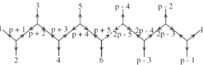
The following calculations are based on the fishbone structure as in Figure 1.
The Steiner Problem is characterized by thep equa-tions below:
$ $ $
, , ,
rp+11+rp+11+rp+1p+2 =0 (1)
$ $ $ ,
, , ,
rj j−1+rj j p− +1+rj j+1=0 p+ ≤ ≤2 j 2p−3 (2)
$ $ $
, , ,
r2p−2 2p−3+r2p−2p−1+r2p−2p =0 (3) where a hat above a letter stands for unit vector which is given by
$
, ,
r r r
R k l l k k l = − r r
andRk,l, with 1≤k,l≤2p- 2 which stands for the Euclidean
distance between the kth Steiner point and the lth leaf or be-tween kth and lth Steiner points, or
Rk l, xk xl xk xl xk xl /
[( ) ( ) ( ) ]
= 1 − 1 2+ 2− 2 2+ 3− 3 2 1 2
(4) Each equation in the set (1)-(3) has as a conse-quence the equality of the angles around a node (Steiner point).
Leti$s be the unit vector in the direction of the sth co-ordinate axis, we have from Eqs. (1)-(3)
x x R x x R x x p s s p p s s p p s p + + + + + − + − + − 1 1 11 1 2 1 2 1 ( ) ( ) , ( ) ( ) , ( ) + + + = =
∑
2 1 2 1 3 0 ( ) , $ s p p s sR i (5)
x x R x x R x j s j s j j j s j p s
j j p
j s ( ) ( ) , ( ) ( ) , ( ) − + − + − − − − + − + 1 1 1 1 x R i j s j j s s + + = =
∑
1 1 1 3 0 ( ) , $ (6) x x R x x R p s p s p p p s p s p2 2 2 3
2 2 2 3
2 2 1
2 2 − − − − − − − − + − ( ) ( ) , ( ) ( ) ,p p s p s p p s s x x R i − − − = + − =
∑
1 2 2 2 2 1 3 0 ( ) ( ) , $ (7)wherep+ 2≤j≤2p- 3.
Equations (4)-(6) can be collected in the expression below δm p p s s p m s m p s m m p
x x R x x R + + + − − + − + − +
1 1 1
11 1 1 1 ( ) ( ) , ( ) , ( ) ,
(
)
(
)
− − + − − − − + = +∑
δ δ m p m s m s m m s m p m s m x x R x x2 2 1
1 1 3 1 1 ( ) ( ) , ( ) − − − − − + − = 1 1
2 2 2 2
2 2 0 ( ) , ( ) ( ) , $ s m m m p p s p s p p s R x x R i δ (8)
where theδmn
is the Kronecker index, withp+ 1≤m, n≤2p -2.
From the linear independence of the unit vectors$i1,
$
i2,...,i$s, we can write
δ ∂ ∂ ∂ ∂ δ ∂ m p p p s
m m p
m s m p m R x R x R + + + − + − + + − 1 11 1
1 2 2
1 , ( ) , ( ) ( ) , ( ) , ( ) , ( ) m m s m
p m m
m
s m
p p p
x R x R x + + − − − + − + 1
1 1 2 2 2 2
1
∂
δ ∂
∂ δ
∂ ∂ 2 2
0 p s − = ( ) (9)
These are 3(p - 2) equations which are enough to solve the problem of determination of 3(p- 2) coordinates of the (p- 2) Steiner points.
We should note that Eq. (9) can be also written as
∂
∂xms R p R p m p Rm m p R p
m m m p
( ) 1, 1 2, 2 , 1 ,
1 2 2 1 + + − + = + − + = + + +
∑
+ 1 2 3 0 p−∑
= (10)
These equations can be also obtained by direct obser-vation of the fishbone tree, Figure 1.
We now go back to Figure 1 and we suppose that for each leaf or node there is an associated “weight”µk,
charac-teristic of the sort of interaction (i.e., electric charges for electrostatic Coulombian interactions) among the atoms whose average positions are given by the positions of nodes and leaves. LetKbe the universal interaction constant. By assuming that the leaves are fixed, we write these potential energy function for this fishbone configuration
U K
R R R
K p p p p p p p = + + + + + + + + + +
µ µ µ µ
µ 1 1 11 2 1 2 2 1 2 , , , 2 3 2 3 3 2 3 2 3 2 2 3 µ µ µ µ R R K R p p p p p p p + + + + − − − + + + , , ... , , , p p p p p p p p R K R − − − − − − − − + + + 2 2 2
2 3 2 2
2 2
1
2 2 1
µ
µ µ µp
p p R2 −2
,
(11)
The positions corresponding to equilibrium are then given by 0 1 1 1 11 2 11 1 = = − + + + + + + ∂ ∂ µ µ ∂ ∂ U
x K R
R x p s p p p p s ( ) , , ( ) ( ) µ ∂ ∂ µ ∂ 2 1 2 2 1 2 1 1 1 2 2 1 ( , ) ( ) , ( ) , , R R x R R p p p s p p p p p + + + + + + + + + 2 1 1 1 2 1 0 ∂ ∂ ∂ µ µ ∂ ∂ x U
x K R
R x p s m s m m m m m m + − − − = = − ( ) ( ) , ,
( ) m
s
m p
m m p
m m p
m s m m R R x R ( ) , , ( ) , ( ) ( + + − + − + − + + µ ∂ ∂ µ 1 1 2 1 1 m m m m s p s p p R x U
x K R
+ + − − − = = − 1 2 1 2 2 2 2 2 3 0 ) ( , ( ) ( ) ∂ ∂ ∂ ∂ µ µ
2 1 2 3
2
2 2 2 3
2 2
1
2 2 1
p p p p p s p p p R x R − − − − − − − − + , , ( ) , ) ( ∂ ∂ µ ) ( ) , ( ) , , ( 2
2 2 1
2 2 2 2
2 2 2 2 2 ∂ ∂ µ ∂ ∂ R x R R x p p p s p p p p p p s − − − − − − + ) (12)
These are 3(p- 2) equations for 3(p- 2) variables and they are enough to describe an equilibrium solution of the fishbone configuration. We restrict the search for equilib-rium to a special tree. This is specified by the equality of the interaction strengths of each node to their adjacent leaves and nodes. If we choose the Coulombian interaction as the only one which is fundamental for this Steiner Tree config-uration, we have,
µ µ ( ) µ µ ( ) µ µ ( ) 1 2 2 2 p p p p p p p p
R R R
+ + + + + + + + = = 1 11 1 1 2 1 2 1 2 , , , 2 − 2 − + 2 µ µ ( ) µ µ ( ) µ µ ( m m m m
m m p m m p
m m m m
R R R
1 1 1 1 1 1 , − , − + , + + = = ) µ µ ( ) µ µ ( 2 2 − , ,
p m p
R R p p p p p p p + ≤ ≤ − = − − − − −
2 2 3
2 2 2 3
2 2 2 3
2 2 1
2 − −
− − = 2 1 2 2 2 2
,p ,
p p p p R ) µ µ ( ) 2 2 (13)
After substituting Eqs. (13) into Eqs. (12), we get 0 1 1 2 1 2 2 1 11 = = − + + + + + + + ∂ ∂ µ µ ∂ ∂ U
x K R
x R R
p
s p
p
p
s p p
( )
,
( ) ,
( )
( 1 2 1 2
1 1 2 0 , , ( ) , ( ) ( ) + = = − + + − + − + R U
x K R
x
p p
m
s m
m p
m m p
m
∂
∂ µ
µ
∂
∂ s m m m m p m m
p
s p
p
R R R
U x K ) , , , ( ) ( − − + , + ) − − − + = = −
1 1 1
2 2
2 2
0 ∂
∂ µ
µ 1
2 2 1
2
2 2
2 2 2 3 2 2 1 2 2
( )
( , ,
,
( ) , ,
R
x R R R
p p
p
s p p p p p
− −
−
− − − − −
∂
∂ ,p)
(14)
This last set of equations can be also written as
0 1 1 2 1 11 1 = = − − + − + + + + ∂ ∂ µ µ δ ∂ ∂ U
x K R
R
x m
s
m m p
m m p m p p p ( ) , , ( ( )
(
)
sm m p
m
s m
p m m
m s m p R x R x ) , ( ) , ( ) + + − + − − + − + ∂ ∂ δ ∂ ∂ δ
1 2 2 1
1
(
1 +)
−− − − + 1 1
2 2 2 2
2 2 ∂ ∂ δ ∂ ∂ R x R x m m m s m
p p p
p s , ( ) , ( ) (15)
The last set of equations is the same set of Eqs. (9), which was written in the form of Eq. (10). This is enough to prove the equivalence of the problems posed by Eqs. (5)-(7) and the problem of potential energy minimization as con-strained by relations (13).
The Steiner Ratio in Euclidean Space
All the molecular structures which we are considering are taken as atomic configurations immersed in the 3-dimensional Euclidean space. However, the interpreta-tion of distances in the internal manifold of the molecule in terms of other geometries is an open problem. In the present work, we assume the strict validity of Euclidean geometry for simplicity. A Steiner Minimal Tree (SMT) is the mini-mal length network if we allow for additional points (nodes) to reach the minimum. A full Steiner Tree has (p- 2) additional points forpgiven points. Figure 1 above which was necessary for our calculations, is an example of a full Steiner Tree. If we do not allow for additional points, the minimal length network is realized in the Minimal Spanning Tree (MST). These two problems are completely different in terms of computational complexity. The former is linear and the later NP-hard.
lSMT = ρlMST (16) We look for the set of points in which we get the greatest lower bound for this function. The lowest upper bound is also important and the present research in 3-dimensional sets has not given any way of merging the two bounds as in the 2-dimensional case, with its value of
ρ = 3 2/ (Du and Hwang, 1990). We think this is a charac-teristic of 3-dimensional space and essential for the struc-ture of a macrobiomolecule.
Nature has many ways of building possible molecular structures with the values of their Steiner Ratios filling this gap. In the following section we shall derive a formula based on a simple modelling like that of Figure 1.
If we choose a configuration of points which is in-spired by molecular conformations,i.e., a helical configu-ration, with points evenly spaced along the helix, the length of the Steiner minimal tree, or its ratio to the corresponding minimal spanning tree, is in a sense a measure of the mini-mum value of potential energy function as was proven in The Potential Energy Minimization and the Steiner Prob-lem. The geometrical constraints to be imposed on the for-mer problem will correspond to thermodynamical requirements used to define a free energy function and to test the stability of the molecular conformation to be mod-elled. We shall develop these ideas in The Buried Area and Geometric Chirality as Constraints - The Optimization Problem.
A Simple Modelling for the Steiner Ratio
Function
The characterization of the Steiner Problem in the form given into Eqs. (5)-(7) has as a consequence the equal-ity of the angles (2π/3) among the edges forming a node. This can be written as (Mondaini, 2002)
$ $ $ $
$ $
, , , ,
, ,
r r r r
r r
p p p p p
j j j j
+ + + + +
−
⋅ = ⋅ = −
⋅
11 1 2 11 1 2
1
1 2
− + − +
− − − −
= ⋅ = −
⋅ =
p j j j j
p p p p
r r
r r r
1 1 1
2 2 2 3 2 2 1 2
1 2
$ $
$ $ $
, ,
, , p−2 2p−3⋅r2p−2p = −
1 2
, $ ,
(17)
Our modelling for the vertices of the spanning tree was
r
rj =(cos jω,sin jω α ω, j ), 1≤ ≤j p (18) which means a configuration of p points evenly spaced along a right circular helix of unit radius.
The results of this modelling were expressed by points evenly spaced along a right circular helix of lesser radius but with the same pitch value (Mondaini, 2001), or
r
r r k r k k
p k p
k =
+ ≤ ≤ −
( ( , )cosω α ω ω α, ( , )sin ω α ω, ),
1 2 2
(19)
From Eqs. (17), we can then write for the radius of the configurations
r( , )
( cos )( cos )
ω α αω
ω ω
=
− −
2 1 1 2 (20)
The last results are enough to write general formulae for the length of the spanning and Steiner trees. We then have the Steiner ratio function for this caseρ(ω,α), as de-fined in Eq. (16), given by
ρ ω α α ω λ
α ω λ
α ω
( , ) ( )( ) ( )
( )
(
= − − + − +
− + +
+
p r p r
p
2 1 3
1 2
2 2 2
2 2
2 2
1 1
2 2
2 2
− +
− +
r r
p
)
( )
λ
α ω λ
(21)
wherer=r(ω,α) is given by Eq. (19) andλ=λ(ω) is
λ=2 1( −cosω) (22)
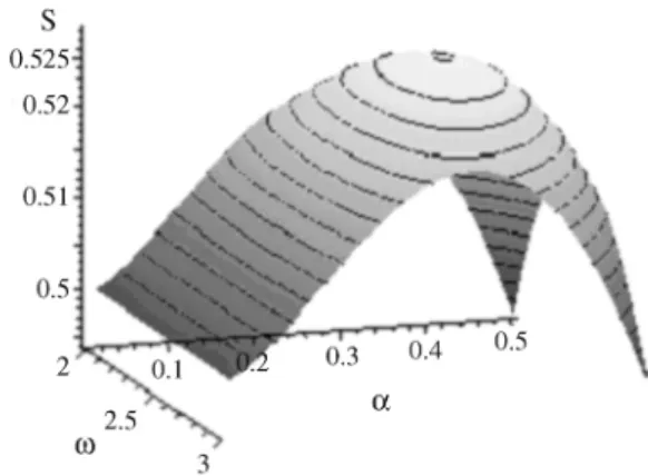
We have used these results for deriving a new upper bound for the Steiner Ratio in E3 (Mondaini, 2003). We now think to use them to propose a definition for measuring geometric chirality of molecular configurations. In order to formulate these ideas, we shall analyze the behavior of an usual definition of chirality in the next section. However, we can put forth that our problem should be better formu-lated when we learn how to restrict the representative of length of the Steiner Tree, i.e., the function ρ(ω, α) (Figure 2). In our analogy of The Potential Energy Minimization and the Steiner Problem, this means how to formulate the problem of potential energy minimization as a constrained problem. The introduction of useful con-straints will then be made in a thermodynamic analogy which completes our construction of a new objective func-tion in The Buried Area and Geometric Chirality as Con-straints - The Optimization Problem.
An Example of Chirality Definition and its
Behavior
According to Kelvin’s definition of chirality, if after translating and rotating a body, we cannot make it coincide with its mirror image, we can say that the body and its im-age are chiral to each other. This definition says just whether an object is chiral or not. It does not specify how chiral an object is to its mirror image. The problem of chirality measure is still an open problem (Gilat, 1994). In the present work we give two examples and we analyze their behavior in a geometric and thermodynamical formu-lation of biomolecular conformation.
Let us consider two helices as representatives of atomic chains in a macromolecule. We takexzas the mirror plane. The helices are then mirror images and the corre-sponding evenly spaced points in them can be written as
r
r
r j j j
j p
r j j j
j
j
D
L
=
≤ ≤
= −
(cos ,sin , )
(cos , sin , )
ω ω α ω
ω ω α ω
1 (23)
The sum of the squared distances between corre-sponding points is then given by
S j p p p
j p
( ) sin sin
sin cos( )
ω ω ω
ω ω
= = − −
=
∑
4 2 2 1
1
(24)
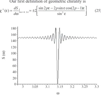
The functionS(ω) has a global minimum atx=π. Its derivative changes from (-) to (+) in this neighborhood (Figure 3). There are serious doubts about the efficiency of the sum of squared distances as a candidate for a measure of chirality (Gilat, 1994). However, in terms of our modelling, the behavior of the function S(ω) does not present any drawbacks.
Our first definition of geometric chirality is
χ ε ω
ε ε ε
ε
ω π ε ±
= ±
= = ± − −
( ) sin sin cos( )
sin dS
d
p p p
2 2 2 2 2 1
(25)
We have, in the neighborhood ofω=π, lim ( ) ( ) limsin( )
cos
ε χ ε ε
ε ε
→ ±
→
= ± − − =
0 2 1 0
2 1
0
p p p (26)
This behavior does not seem to be enough to discard this definition as a reasonable representative of chirality’s measure as far as our modelling is concerned.
Our second example of a candidate function for char-acterizing geometric chirality will be given by a pseudo-scalar quantity (de Gennes, 1992). We take as a representative, the volume of the tetrahedra cells formed by the edges of lengthRj, j+1,Rj+1, j+2,Rj+2, j+3, 1≤j≤pin the
structure of Figure 1 and we have
χ ω α( , )= 1 ⋅ × = αωsinω( −cosω) 6
2
3 1
2
r r r
C A B (27)
where
r r r
A=rj+1−rj,
r r r
B=rj+2−rj,
r r r
C=rj+3−rj andrrj, rrj+1,
r
rj+2,rrj+3 are obtained from
r
rj l+ =(cos(j+l) ,sin(ω j+l) , (ω j+l)αω), l=0 1 2 3 (28), , , The advantage of takingχ(ω,α) as given in Eq. (27) as the representative of geometrical chirality will be seen in the next section (Figure 4).
The Buried Area and Geometric Chirality as
Constraints - The Optimization Problem
One of the essential contributions to the understand-ing of molecular interactions and their thermodynamical description was the discovery of the influence of the area of intramolecular cavities in the free energy calculations. These cavities (Rashin, 1984) are substructures formed by non-covalent processes with a free energy attribution. It is a kind of hydrophobic effect in the molecular structure caused in part by the non-polar Van der Waals interaction. This contribution to the free energy is usually called the
Figure 3- The squared sum of distances on a candidate for geometric chirality,p= 300.
cavitation free energy. It is considered to be a good descrip-tion of this hydrophobic effect by keeping the cavities open in order to bury partially the side chains of the amino acids in a protein. It can be given by
∆GCav = γ∆A (29)
whereγis the interfacial tension and∆A the area measure of the cavity. The consideration of this new free energy contribution corresponds also to molecular stability.
We consider it to be representative of the area mea-sure, the area of helicoidal surface between the helix of unit radius and the internal helix of radiusr(ω,α) by unit of po-lar angleω, in the modelling of A Simple Modelling for the Steiner Ratio Function. We have, from the Monge repre-sentation of the area element
dS z
x
z
y dxdy
= +
+
1
2 2
∂ ∂
∂ ∂
withz=αarctan(y/x);x2+y2=r2we get
∂
∂ω ω α ω αα
S
s r dr
r
= ( , )=
∫
+ ( , )2 2
1
(30)
wherer(ω,α) is given by Eq. (20).
We then get for the measure of area by unit of polar angle (Figure 5),
s( , )ω α α α ln α M( )
α ω
= + + + +
−
1
2 1
1 1
2 2
2
(31)
where
(
)
M( )ω =u u2+ +1 ln u+ u2+1 and
u=u =
− −
( )
( cos )( cos )
ω ω
ω ω
2 1 1 2
We are now able to formulate a thermodynamically inspired optimization problem. Since we are planning to describe the transition to more stable structures in the pro-cess of molecular formation with the contribution of chirality and this one is represented by a measure of vol-ume, the objective function to be minimized is a Gibbs-like free energy or,
H=ρ ω α( , )+Pχ ω α( , )−Ts( , )ω α (32) andρ,χ,sare given by Eqs. (21), (27) and (31), respec-tively.PandTare Lagrange multipliers.
The structure of an algorithm can be now planned as
∆nH=∆nρ+Pn∆nχ −Tn∆ns (33)
and we have for consecutive steps
∆ ∆ ∆
n n n
n n n
n s s s n n
+ + +
= − = − = − 1
1
1
ρ ρ ρ ω α χ χ χ ω α
ω α
( , ) ( , ) ( , )
(34)
with (ωn,αn) as the point determined in the previous step of
the calculation.
Concluding Remarks
Our basic aim in this work was to derive an optimiza-tion process in order to minimize the Steiner Ratio funcoptimiza-tion. We think that this process will correspond to the work done by evolution in its search for more stable structures. It should be noted that we have used the area measure by unit of polar angle s(ω,α) as the contribution to Gibbs free en-ergy Eq. (32) in this thermodynamics analogy. In order to introduce the enthalpy function which is of the formU+ PV, whereUis internal energy andP,Vare pressure and volume, respectively, we have used our second example of geometric chirality which is given by the volume of the ele-mentary cells of the molecular modelling configuration in-troduced in the last section. The minimization of the free energy of macromolecular structures, with a geometrical characterization of the terms corresponding to volume and conformational entropy seems to be a reasonable scheme. Nevertheless, we have to improve these ideas by taking into consideration a more realistic modelling. This could be based on the existence of peptide planes in the macromolecular conformation of a protein. We expect to have a greater value for the lower bound of the new Steiner Ratio Function. We also expect to create a function which is as reliable as the present one in its precision at reproducing, up to 38 decimal places, the results advanced by direct cal-culation with the assumption of symmetry of the molecular conformation.
Acknowledgements
We are indebted to an anonymous referee for some enlightened observations which have contributed to the im-provement of this work.
References
Bookstein FL (1978) The measurement of biological shape and shape space change. Lecture Notes in Biomathematics, 24 pp.
Cieslik D (1998) Steiner Minimal Trees. Kluwer Acad Publ. Du D-Z and Smith WD (1996) Disproofs of Generalized-Pollak
Conjecture on the Steiner Ratio in three or more dimensions. Journ Comb Theory A74:115-130.
Du D-Z and Hwang FK (1990) The Steiner Ratio Conjecture of Gilbert and Pollak is true. Proc Nat Acad Sci 87:9464-9466. de Gennes PG (1992) Simple views on condensed matter. Series
in Modern Condensed Matter Physics, v 4.
Gilat G (1994) On quantifying chirality - Obstacles and problems towards unification. J Math Chem 15:197-205.
Gilbert EN and Pollak HO (1968) Steiner minimal trees. SIAM J Appl Math 16:1.
Mondaini R (2001) The minimal surface structure of
biomolecules. Proceedings of the First Brazilian Sympo-sium on Mathematical and Computational Biology, ed E-papers Ltda, pp 1-11 and references therein.
Mondaini R (2002) The disproof of a conjecture on the Steiner Ra-tio in E3and its consequences for a full geometric descrip-tion of macromolecular chirality. Proceedings of the Second Brazilian Symposium on Mathematical and Computational Biology, ed E-papers Ltda, pp 101-177.
Mondaini R (2003) The Steiner Ratio and the homochirality of biomacromolecular structures. Nonconvex Optimization and its Applications Series, Kluwer Acad Publ 74:373-390. Mondaini R (2004) A Dilemma on the Euclidean Steiner Ratio for
helical point sets - (in preparation).
Rashin AA (1984) Buried surface area, conformational entropy, and protein stability. Biopolymers 23:1605-1620.