i
Stjepan Tomislav Rajcic
ii
SPATIAL ANALYSIS OF CRIME EVOLUTION IN PORTUGAL
BETWEEN 1995 AND 2013
Supervised by:
Prof. Dr. Paulo Gomes
Co-supervised by:
Prof. Dr. Ana Cristina Costa
Prof. Dr. Jorge Mateu
iii
ACKNOWLEDGMENTS
I would like to express my gratitude to Prof. Dr. Paulo Gomes for the supervision, help and suggestions during the work in this thesis. His suggestions were of great help and importance to me. I am also very grateful to him for introducing me into data analysis field during the course held at Nova IMS.
iv
SPATIAL ANALYSIS OF CRIME EVOLUTION IN PORTUGAL
BETWEEN 1995 AND 2013
ABSTRACT
v
KEYWORDS
Crime evolution
Spatial data analysis
Multidimensional data analysis
STATIS
vi
ACRONYMS
PCA - Principal component analysis
vii
INDEX OF TEXT
ACKNOWLEDGMENTS ... iii
ABSTRACT ... iv
KEYWORDS ... v
ACRONYMS ... vi
INDEX OF TABLES ... ix
INDEX OF FIGURES ... x
1. Introduction ... 1
2. Methods ... 4
2.1. Principal component analysis ... 4
2.2. STATIS ... 7
2.2.1. Interstructure analysis ... 8
2.2.2. Finding the compromise ... 11
2.2.3. Intrastructure analysis ... 12
2.2.4. Trajectories of observations ... 13
2.3. Clustering techniques ... 14
2. 3. 1. Hierarchical clustering ... 15
2. 3. 2. K-means algorithm ... 15
2.4. Trajectory classification techniques ... 15
2.5. Spatial statistical techniques –Moran’s index ... 18
3. Data description ... 19
3.1. Data structure ... 19
3.2. Variable description ... 20
4. Exploratory data analysis ... 23
5. Results and discussion ... 24
5.1. Global analysis ... 24
5.1.1. Crime evolution in Portugal ... 24
5.1.2. Interstructure analysis of data tables ... 31
5.2. Spatial analysis of crime evolution in Portugal ... 33
5.2.1. Definition of the compromise ... 33
5.2.2. Interpretation of compromise ... 34
5.2.3. Interpretation of compromise position of NUTS III regions ... 36
5.2.4. Trajectories of NUTS III regions ... 47
viii
6. Conclusion ... 56
Bibliographic references ... 1
ANNEX 1 - GLOBAL CRIME EVOLUTION IN PORTUGAL DATA AND SUMMARY STATISTICS ... 3
ANNEX 2 - CRIME EVOLUTION IN PORTUGESE NUTS III REGIONS DATA FOR THE 1995-2013 PARIOD AND SUMMARY STATISTICS ... 7
ANNEX 3 - EIGENVALUES ASSOCIATED WITH PERCENTAGE OF INERTIA (PCA) ... 46
ANNEX 4 - RV COEFFICENTS (STATIS) ... 48
ANNEX 5 - NORMS (STATIS) ... 50
ANNEX 6 - MATRIX S (STATIS) ... 52
ANNEX 7 - FIRST TWO INTERSTRUCTURE COMPONENTS (STATIS – INTERSTRUCTURE) ... 54
ANNEX 8 - COMPROMISE AND EIGENVALUES WITH ASSOCIATED WITH PERCENTAGE OF INERTIA (STATIS – COMPROMISE) ... 56
ANNEX 9 - CORRELATION BETWEEN VARIABLES AND COMPROMISE PRINCIPAL COMPONENTS – VALUES ... 59
ANNEX 10 - CORRELATION BETWEEN VARIABLES AND COMPROMISE PRINCIPAL COMPONENTS – TRAJECTORIES ... 62
ANNEX 11 - PERCENTAGE OF INTRACLASS INERTIA FOR HIERARHICAL CLUSTERING METHODS (CLUSTERING BASED ON COMPROMISE POSITION) ... 68
ANNEX 12 - CLASSES OF NUTS III REGIONS (CLUSTERING BASED ON COMPROMISE POSITION) ... 70
ANNEX 13 - TRAJECTORIES OF NUTS III REGIONS ... 72
ANNEX 14 - PERCENTAGE OF INTRACLASS INERTIA FOR HIERARHICAL CLUSTERING METHODS (CLUSTERING BASED ON TRAJECTORIES) ... 83
ANNEX 15 - CLASSES OF NUTS III REGIONS (CLUSTERING BASED ON TRAJECTORIES) ... 85
ix
INDEX OF TABLES
Table 1 Factorial coordinates for trajectories……….….……16
Table 2 Summary statistics for the set of 19 data tables ………..……23
Table 3 Absolute and relative contributions of variables on the 1st plane………….…….…25
Table 4 Principal components and their absolute and relative contributions…………...……27
x
INDEX OF FIGURES
Figure 1 Four typical cases of interstructure relations………12
Figure 2 Trajectories with: similar position and different evolution (2 a), and similar evolution and different position (2 b)………..16
Figure 3 Percentage of inertia explained by each component……….25
Figure 4 Correlation of the variables with principal components……….26
Figure 5 Crime evolution represented on the 1st principal plane……….26
Figure 6 Interstructure. ………32
Figure 7 Compromise position of NUTS III regions on the 1st principal plane………..38
Figure 8a Values of 1st PC……….………..41
Figure 8b Values of 2nd PC………....….42
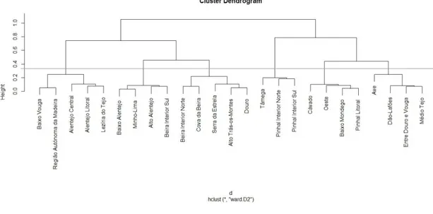
Figure 9 Dendogram for ward’s method………..43
Figure 10 Average values of principal components for classes 1-6……….44
Figure 11 Average values of principal components for classes 7-11………45
Figure 12 Map of NUTS III regions classified by their compromise position………..……..46
Figure 13 Dendogram for ward’s method………..………..52
1
1. Introduction
Changes over time in the levels and patterns of crime have significant consequences that affect not only the criminal justice system but also other critical policy sectors. Descriptive information and explanatory research on crime trends across the nation that are not only
accurate but also timely are pressing needs in the nation’s crime-control efforts. Without useful and reliable information, national and local policy makers are not able to implement effective policies for crime prevention, properly evaluate the effectiveness of policy interventions, and combat crime in general (Goldberger & Rosenfeld, 2008).
For these reasons there is a strong need to conduct crime analysis. Crime analysis includes analysis of crime trends and patterns. It plays an important role in the human society, especially in crime prevention and devising solutions to crime problems. Since the birth of criminology, researchers have employed a variety of quantitative methods to describe the origins, patterning, and response to crime and criminal activity, and this line of research has generated important descriptive information that has formed the basis for many criminological/criminal justice theories and public policies (Piquero & Weisburd, 2010).
The objective of this survey is to make a spatial analysis of crime evolution in Portugal between 1995 and 2013 using various quantitative techniques. So, we will focus on both spatial and temporal aspects of the crime. Our objective it is only to make a descriptive spatial and temporal analysis of crime trends, so we will not focus on examining the factors that appear to have been influential in driving crime trends. Also we will try to focus on all main crime types. We haven't found any scientific work with an integrated spatial and temporal analysis of all main crime types and patterns in a perennial period. So, the motivation for this survey was to describe and present main spatial and temporal crime trends in Portugal since a global integrated analysis was not conducted before.
Spatial crime patterns will be analysed on the level of NUTS III regions as minimal spatial units, while temporal crime patterns will be analysed on the level of years as minimal temporal units. The crime data are represented by a set of 19 data tables, where each table contains data for each year of the 1995-2013 period. In each table NUTS III regions of Portugal are observations, and crime rates of various crime types are variables. The data are provided by Portuguese Ministry of Justice.
2
represent a multidimensional data set in lower dimension space. In our work principal component analysis will be used to analyse global crime evolution patterns in Portugal.
However, the base of this survey will be STATIS method which is based on the principals of PCA. STATIS is a descriptive data analysis technique whose objective is to summarize main characteristics of data set, and to represent the summary combining statistical analysis with visual methods. It is used to perform a joined analysis of the set of quantitative tables. STATIS will be used to analyse the set of 19 tables with spatially referenced crime data. This survey will be focused on general analysis of main crime trends, so we will not be analysing each table separately.
In the last years STATIS method has been used to perform a number of three-way analysis in various distinct fields. In the industry it is applied to monitoring of the evolution in time of batch processes (Gourvénec et al., 2006) and development of multivariate control charts for monitoring non-linear batch processes (Marcondes Filho et al., 2011). It is also applied to environmental data in order to investigate transport processes inside karst aquifer of the western Paris (Fournier et al., 2008). STATIS was also used to characterize the internal molecular motions and conformational states of flexible molecules from molecular dynamics simulations (Coquet et al., 1994). It was also used to analyse the travel modes in Brazilian cities (Coelho Barros et al, 2009).
Few extensions of STATIS method are also developed. These include X-STATIS or
partial triadic analysis (PTA) which is used when all data tables collect the same variables measured on the same observations (e.g., at different times or locations), COVSTATIS, which handles multiple covariance matrices collected on the same observations, DISTATIS, which handles multiple distance matrices collected on the same observations and generalizes metric multidimensional scaling to three way distance matrices, Canonical-STATIS (CANOSTATIS), which generalizes discriminant analysis and combines it with DISTATIS to analyse multitable discriminant analysis problems, power-STATIS, which uses alternative criteria to find STATIS optimal weights, ANISOSTATIS, which extends STATIS to give specific weights to each variable rather than to each whole table, (K + 1)-STATIS (or external
-STATIS), which extends STATIS (and PLS-methods and Tucker inter battery analysis) to the analysis of the relationships of several data sets and one external data set, and double-STATIS (or DO-ACT), which generalizes (K + 1)-STATIS and analyses two sets of data tables, and
3
STATIS will be the base of this spatial-temporal analysis of crime, but some other auxiliary statistical techniques will also be used to analyse the outputs of STATIS. These include trajectory classification methods, clustering and spatial statistical techniques. Trajectory analysis techniques are also used in criminology. One of prominent examples includes criminological analyses of the progression and causes of criminality over life stages or of time trends of reported crime across geographic locations (Piquero & Weisburd, 2010). Trajectories of observations are built in the last step of STATIS, so trajectory classification methods will be used in this survey. Spatial statistical techniques are unique in that they were
developed specifically for use with geographic data. They differ from originally “non-spatial” techniques like STATIS which can be applied on any data set (including spatial data). There is a wide variety of spatial statistical techniques which can be used in crime analysis. One of
widely used techniques is Moran’s Index (Piquero & Weisburd, 2010), which will also be used in this survey.
The crime analysis will be performed using R software for the statistical analysis and ArcGIS for the spatial analysis and geospatial representation of the data.
The thesis consist of few sections. In the introduction section background to the study, motivation, methods and objectives of the study were briefly presented were presented. In the methods section techniques used in the analysis have been presented: principal component
analysis, STATIS, clustering methods, trajectory classification methods and Moran’s Index.
4
2. Methods
In this survey few statistical techniques will be used to analyse spatial crime evolution patterns in Portugal between 1995 and 2013. These include principal component analysis, STATIS technique, trajectory classification techniques, cluster analysis and spatial statistical techniques.
2.1. Principal component analysis
Principal component analysis (PCA) is a statistical procedure that uses an orthogonal transformation to convert a set of correlated variables into new variables called principal components. The number of principal components is less than or equal to the number of original variables. The objective of PCA is to extract maximal amount of information from the data table and present it in a graphical form. In our survey we have applied PCA using denomination and methodology proposed by Dazy & Le Barzic (1996).
Before explaining principals of PCA it is important to define the data set and its main
features. Let’s denote with Y a matrix associated with the table with n observations and p
variables:
Y =
[
𝑦11 ⋯ 𝑦1𝑗 ⋯ 𝑦1𝑝
⋮ ⋱ ⋰ ⋮
𝑦𝑖1 𝑦𝑖𝑗 𝑦𝑖𝑝
⋮ ⋰ ⋱ ⋮
𝑦𝑛1 ⋯ 𝑦𝑛𝑗 ⋯ 𝑦𝑛𝑝]
Each variable from the table can be associated with a vector yj = [𝑦1
1
⋮ 𝑦𝑛𝑗
], while each observation
can be associated with a vector ei=[𝑦𝑖1… 𝑦𝑖𝑝].
In the beginning of the analysis it is necessary to attribute a weight to each observation. These weights are represented by the weight matrix:
D = [𝑝1 ⋱ 0
0 𝑝𝑛
5
Centre of gravity of the data matrix associated with the weights is a vector g defined by:
g = [𝑦̅
1
⋮
𝑦̅𝑝] where 𝑥̅
𝑗 = ∑ 𝑝 𝑖𝑥𝑖𝑗 𝑛 𝑖=1
Centre of gravity can be seen as a generalization of the mean.
Usually PCA is not applied on the original data matrix, but on the centred data matrix. We can define a centred table X, associated with the initial table Y, as:
X = [⋱ 𝑥𝑖𝑗= 𝑦𝑖𝑗− 𝑦̅𝑗 ⋰
⋰ ⋱
] =
[
𝑥11 ⋯ 𝑥1𝑗 ⋯ 𝑥1𝑝
⋮ ⋱ ⋰ ⋮
𝑥𝑖1 𝑥𝑖𝑗 𝑥𝑖𝑝
⋮ ⋰ ⋱ ⋮
𝑥𝑛1 ⋯ 𝑥𝑛𝑗 ⋯ 𝑥𝑛𝑝]
.
We can also define a matrix of variance and covariance V, and a matrix of correlation R, both associated with the initial matrix as:
V =
[
𝑠12 ⋯ 𝑠1,𝑖 ⋯ 𝑠1,𝑝
⋮ ⋱ ⋯ ⋮
𝑠𝑖,1 𝑠𝑖2 𝑠𝑖,𝑝
⋮ ⋱ ⋮
𝑠𝑝,1 ⋯ 𝑠𝑝,𝑖 ⋯ 𝑠𝑝2]
where 𝑠𝑗2 is covariance of a variable j defined: 𝑠𝑗2=
∑𝑛𝑖=1𝑝𝑖(𝑥𝑖𝑗)2, and 𝑠𝑗𝑗′variance of variables j and j’ defined: 𝑠𝑗𝑗′= ∑𝑛𝑖=1𝑝𝑖𝑥𝑖𝑗𝑥𝑖𝑗′.
R =
[
1 𝑟1,2 ⋯ 𝑟1,𝑝
𝑟2,1 ⋱ ⋮
⋮ ⋱ 𝑟𝑝−1,𝑝
𝑟𝑝,1 ⋯ 𝑟𝑝,𝑝−1 1 ]
.
Each variable can be seen as an element of a vector space called variable space. In variable space we can define a metric D which enables us to calculate distances between variables. This metric is the weight matrix D.
6
M=Ip=[
1 0
⋱
0 1]
.
In case when there is a need to standardize the data, we use matrix:
𝑀1/𝑠2 = [
1 𝑠12
⁄ 0
⋱
0 1 𝑠
𝑝2
⁄ ]
.
The squared distance between two observations ei and ej is defined by a relation:
d2(e
i, ej )=( ei - ej)’M(ei - ej)= || ei − 𝑒𝑗 ||M2
Inertia Ig of the set of points is defined as an average pondered squared distance of points from their centre of gravity:
Ig=∑𝑛𝑖=1𝑝𝑖(ei − g)’M(ei − g) = || ei − g ||M2 Inertia has a property:
Ig=Tr(MV), where Tr(A) is a trace of the matrix A.
Finally, one "survey" is defined as a triplet: (X,M,D) where X is a centred data matrix, M metric on the observation space and D metric on a variable space.
The main idea of PCA is to obtain a close representation of the set of initial observations in the sub-space of the lower dimension. When projecting the observations in a lower dimension space it is necessary to take into consideration the fact that the distances between observations have to suffer the least possible deformation in the projection. This means that in a subspace of the dimension k the average value of squared distances between projected observations has to be the highest possible; the inertia of the projected cluster has to be maximal. It can be proved that the subspace of the dimension k is generated with k eigenvectors of the matrix VM associated with k highest eigenvalues:
VMµ=µπ.
In the context of PCA these eigenvectors µ1, … µk are orthogonal vectors generating so-called principal axes. Inertia explained by each principal axis is equal to the value of eigenvalues π1
, … πk associated to it. Finally, principal components are the new variables ct in a subspace which is generated by the eigenvectors (principal axis) and defined by:
7
After finding principal axes, principal components, and eigenvalues, the obtained results have to be interpreted. Principal axes can be interpreted by calculating the correlation between principal components and variables from the initial table. They are usually represented with the circle of correlations.
When a principal component shows a strong correlation with a variable it means that observations with high positive component values have variable values notably superior then the average.
It is also possible to calculate the absolute contribution CTA of the observation i to the principal axis k which is defined by:
𝐶𝑇𝐴𝑖𝑘= 𝑝𝑖(𝑐𝑖𝑘)2
𝑙𝑘 .
Also, it is possible to calculate relative contribution CTR of the observation i to the principal axis k:
𝐶𝑇𝑅𝑖𝑘= (𝑐𝑖
𝑘)2
𝑥𝑖′𝑀𝑥𝑖.
Relative contribution of an observation i is equal to the cosines of the angle between the principal axis and vector ei representing an observation. Relative contribution represents the quality of the representation of an observation on that axis (or plane); if it close to 1 the representation is very good.
The basic idea of the supplementary points technique is to place additional observations and/or variables in the Euclidian image. These additional observations and variables are called supplementary observations and variables. They were not used when PCA was performed on the data table, but they may contribute to the interpretation.
2.2. STATIS
8
our survey we have applied STATIS using denomination and methodology proposed by Dazy & Le Barzic (1996) and Lavit (1988.).
STATIS technique is designed to analyse the set of T data tables (plot X). Tables 1, ... t, ... T represent a phenomena measured on the set of same observations in different circumstances (where variables may be different from one table to another). The analysis is performed on T studies where each study t is defined with a triplet (Xt, Mt, D)t (as described in 2.1.). The weight given to each observation has to be same for all the tables; the metric D is constant, while metric M may wary depending is there is a need to standardize the data.
STATIS uses scalar products to analyse the data. Scalar product can be defined for each pair of observations ei and ej. Scalar product is a bilinear symmetric form wij defined by wij=<ei,ej> =eiMtej. A scalar product between two objects can be seen as a measure of association between them.
When applying STATIS it is necessary to represent each study (Xt, Mt, D)t with one object. This object, denoted Wt, is the matrix of scalar products between observations in a table. It is defined by Wt=XtMXt’. The matrix Wt can be seen as a table of associations between the observations in a table. However, Wt can't be considered as a table of similarities because the values in the diagonal are generally not equal.
Like other descriptive methods designed for evolution data, STATIS has an analytical structure which consists of:
-interstructure analysis
-finding a compromise
-intrastructure analysis
- plot of trajectories of observations
2.2.1. Interstructure analysis
9
between tables represented by Wt. Hilbert-Schmidt scalar product between objects Wt and Wt' is defined:
<Wt | Wt'>HS = Tr (DWtDWt')
It represents a measure of association between two tables.
It is also possible to define the norm of an object Wt, denoted ||Wt||, where squared norm is defined by: ||Wt||2HS = <Wt | Wt>HS. In case when tables have significantly different norms it is strongly recommended to represent the "surveys" as normed objects Wt/||Wt||HS instead of Wt. Objects with higher values strongly affect the compromise structure in the further analysis, which can be dangerous for the interpretation of results.
The Hilbert-Schmidt scalar products can be interpreted thanks to the interpretation of an expression ||Wt - Wt'||HS. Expression||Wt - Wt'||2HS represents pondered sum of squares of differences between the scalar products between observations from the tables t and scalar products between observationsfrom the tables t':
||Wt - Wt'||2HS =∑ ∑ 𝑝𝑖𝑝𝑗[< 𝑒𝑖(𝑡), 𝑒𝑗(𝑡)>𝑀𝑡− < 𝑒𝑖(𝑡 ′)
, 𝑒𝑗(𝑡′)>𝑀𝑡′]2 𝑛
𝑗=1 𝑛
𝑖=1 .
We can denote with S the matrix of Hilbert-Schmidt scalar products between "surveys" represented by Wt. Matrix S is defined by:
S=[⋱ 𝑆𝑡𝑡′=< 𝑊𝑡|𝑊𝑡′>𝐻𝑆 ⋰
⋰ ⋱]
.
The matrix of Hilbert-Schmidt products can be seen as a matrix of associations between "surveys". However, it can’t be considered as a table of similarities because the values
in the diagonal are generally not equal.
Another measure of association between two studies t and t' is the so-called RV coefficient (Escouffier, 1973). RV coefficient can be seen as a multivariate generalization of
the correlation coefficient. It is defined as a Hilbert-Schmidt product between two normed objects:
RV (t, t')=〈 𝑊𝑡
||𝑊𝑡||𝐻𝑆|
𝑊𝑡′
||𝑊𝑡′||𝐻𝑆〉HS.
Values of RV coefficients can range from 0 to 1. An RV coefficient enables us to calculate the distance between two normed objects:
d( 𝑊𝑡
||𝑊𝑡||𝐻𝑆|
𝑊𝑡′
||𝑊𝑡′||𝐻𝑆)=√2(1 − 𝑅𝑉(𝑡, 𝑡
10
If RV(t,t') = 1 then (Wt/||Wt||HS ) = (Wt'/||Wt'||HS ). If RV(t,t') = 0 and M=Ip, then the values of covariance between variables from the table t and the variables from table t' are equal to 0.
After calculating the relations between tables, it is possible to represent them on the Euclidian image. This means that it is possible to plot the interstructure relations. In order to do this it is necessary to give a weight qt to each study. Weights are represented with the matrix:
Q=[𝑞1 ⋱ 0
0 𝑞𝑡
].
One of main ideas of STATIS is to represent the table of scalar products between objects in Euclidean space of lower dimension so that the scalar products can be well restored. The Euclidean image of n individuals associated to scalar products wij is a set of points M1, ... Mn and a point O of the affine Euclidian space which resituates scalar product in the form:
for every i,j e {1,... n} <OMi, OMj > = wij
The same property applies to the Hilbert-Schmidt product <Wt | Wt'>HS .
Euclidean image of data tables associated with matrix of scalar products S is obtained by performing a specific version of PCA on the matrix of scalar products S where SQ matrix corresponds to VM matrix of the "standard" PCA. So, it is necessary to calculate eigenvectors and eigenvalues of matrix SQ. The eigenvectors represent axes which form the new Euclidean space. In this case principal axes are not interpretable, so in practice only first two PC are taken into consideration. If f1, ... fn are eigenvectors of matrix SQ and t1, ... tn eigenvalues associated to them, then first two PC can be calculated by:
√𝑡𝑖𝑓𝑖.
The distance between two points Mt and Mt' in the 1st principal plane is the best possible approximation of the Hilbert-Schmidt distance between objects representing two tables t and t'.
11
2.2.2. Finding the compromise
The objective of finding a compromise is to find a commune and unique structure which explains and detects the most important tendencies of the studied phenomenon. Compromise can be seen as a global summary of the tables. The idea is to find this commune structure without analysing separately each table.
The compromise W is an object defined as pondered average of all objects Wt:
W =∑𝑇𝑖=1𝑎𝑡𝑊𝑡.
It has a property that it is an object which is mostly correlated with all Wt objects. It can be proved that W will be mostly correlated with all Wt objects when:
at = 1/√𝑜1(∑𝑇𝑡=1𝑞𝑡√𝑆𝑡𝑡)𝑞1𝑓1(𝑡) where o1 is the first eigenvalue of the matrix WtD.
When interpreting the compromise it is important to consider the coefficients at; tables associated with higher at will have a higher contribution to the compromise.
Compromise can also be plotted on Euclidean image of intrstructure. It is situated on the 1st principal axis, at the distance ||W||HS from O. Interstracture plot is important when analysing if compromise W is a good "resume" of data tables. Objects Wt with more elevated norms have significantly higher associated at coefficients.
12
Figure 1 Four typical cases of interstructure relations
In case when Wt objects have significantly different norms (Figure 1 a) it is strongly recommended to work with normed objects. In case when studies are not correlated (Figure 1 b) (angles between vectors representing studies are large) compromise will not represent a good "resume". On the other hand, when studies are very well correlated (Figure 1 c) (angles between vectors representing studies are small) the compromise will represent a good "resume". Also if there are outliers -tables that are not correlated with majority of other tables - then these tables will not have a good representation on compromise (Figure 1 d).
2.2.3. Intrastructure analysis
13
of intrastructure analysis the compromise positions of observations are obtained in the compromise plane and interpreted. In the second part of analysis the trajectories of observations are obtained in the compromise plane and interpreted.
In this stage of analysis it is possible to represent each observation i by one vector and point Ai - its compromise position. Compromise position of observations is obtained by performing a specific version of PCA on compromise matrix of scalar products W where WD matrix corresponds to the VM matrix of the "standard" PCA. So, it is necessary to calculate eigenvectors and eigenvalues of the matrix WD. The eigenvectors m1, .... mn represent principal axes which of the new Euclidean space, while eigenvalues l1, ... ln associated to eigenvectors represent inertia associated to each axis. Principal components representing compromise position of observations are calculated by:
1
√𝑙𝑘𝑊𝐷𝑚𝑘
Compromise position of observations describes their average position in the set of tables. The distance between two points Ai and Aj in compromise plane represents the pondered average distance d between observations i and j in the set of tables:
d2
A1A2=∑𝑇𝑡=1𝑎𝑡||𝑒𝑖(𝑡)− 𝑒𝑗(𝑡)||2.
Like in PCA, the interpretation of principal axis can be obtained by calculating the values of correlation between principal components and variables from each original table. In the way trajectories of variables can be plotted in the correlation plane.
2.2.4. Trajectories of observations
The finest analysis is conducted by placing each observation from each table in the compromise plane using the method of supplementary points. Each point A1(t), ... An(t) represents different positions of observation n in the data tables T on the compromise plane. Coordinates of observation n in the table t on the axis k are calculated by:
1
√𝑙𝑘𝑊𝑡𝐷𝑚𝑘.
14
Compromise position of the observation i, represented by the point Ai, is the canter of gravity of points Ai(1), ... Ai(T) (representing the position of the observation i in different tables) pondered by the corresponding coefficients at.
In the case of evolution data it is possible to represent observations with trajectories. In this case trajectories of observations and variables represent the evolution of phenomena as it is described by each table. In the case of non-evolution data trajectories represents only similarities between observations and variables as they are described by each table.
At the end it is important to note that, like in PCA, technique of supplementary points can be also used in STATIS.
2.3. Clustering techniques
Cluster analysis or clustering is the task of grouping a set of objects in such a way that objects in the same group (called a cluster) are more similar to each other than to those in other groups (clusters). Typically when applying clustering on a data table the observations (lines) described by the set of variables or characters are being grouped into clusters.
When applying clustering techniques it is important to optimize different types of inertia. If we partition a set of n points into k groups then we can denote:
g1, ...gk; centres of gravity of k groups
I1, ... Ik; interties of k clusters
Total inertia I of the set of all n points is equal to:
I = Iw + Ig, where Iw is the intraclass inertia which is equal to the sum of inertias of all clusters, and Ig is the interclass inertia of the set of k centres of gravity. One of objectives of clustering is to obtain such a partition where Iw is minimal (so that all the clusters could be as much as homogenous as possible) and Ig maximal; this means that the ratio Iw/I has to be maximal (Dazy & Le Barzic, 1996).
15
2. 3. 1. Hierarchical clustering
Hierarchical clustering is a clustering method whose objective is to build a hierarchy of clusters. There are various versions of hierarchical clustering, but here we will consider techniques where each observation starts in its own cluster, and then the pairs of clusters are merged into new clusters based on their similarity until the complete hierarchy is established. The results of hierarchical clustering are usually presented in a dendrogram. Similarity and dissimilarity can be measured by calculating distances between sets of observations. In order to define the distance we have to define a metric. Besides Euclidian distance, there are different kinds of distances (i.e. Ward distance, Manhattan distance etc.) with their corresponding metrics. Linkage criteria defines the distance used in the clustering. In our case we will use single, complete, average and ward linkage criteria. (Lebart et al., 2002)
When applying hierarchical clustering the observations are not required; it is enough to provide a matrix of distances between observations.
2. 3. 2. K-means algorithm
K-means algorithm is a clustering method which aims to partition n observations into k clusters where each observation belongs to the cluster with the nearest mean. In the first step points c1, ...ck are usually randomly placed in the set which has to be parted. There are few initialization methods which define how initial seed will be placed. Each observation in the set is assigned to the cluster closets to each cj. In the second step the initial seeds are replaced with the centres of the gravity of the corresponding clusters and process of assigning observations to clusters is repeated. The algorithm has converged to the optimum when the seeds stop changing. There is no guarantee that the global optimum (where ratio Iw/I is maximal) will be found using k-means.
2.4. Trajectory classification techniques
16
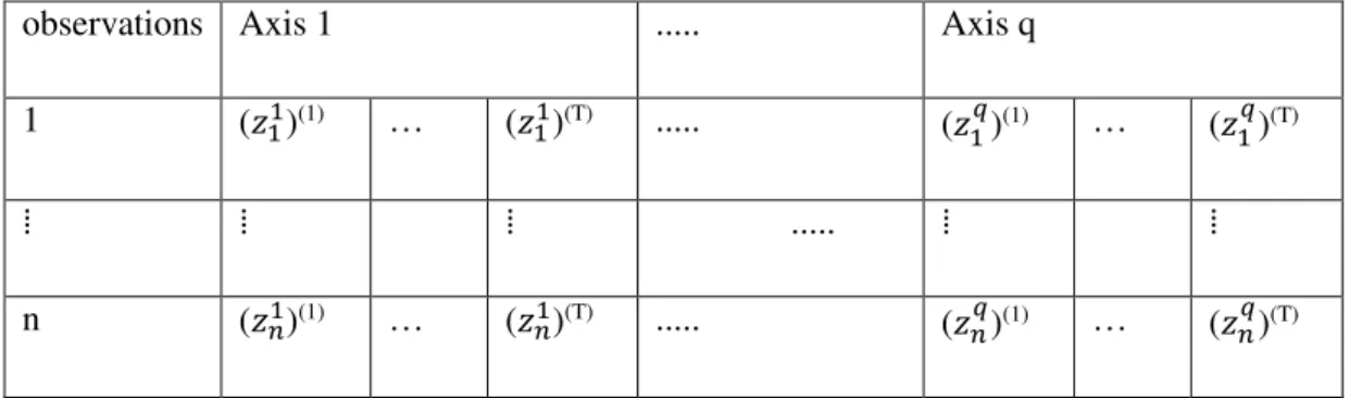
It is possible to represent trajectories using their factorial coordinates (table 1) where
q is the number of axes. (𝑧𝑖𝑗)(t) represent the coordinate of an observations i on the factorial axes j in the point t.
observations Axis 1 ... Axis q
1 (𝑧11)(1) … (𝑧11)(T) ... (𝑧1𝑞)(1) … (𝑧1𝑞)(T)
⁞ ⁞ ⁞ ... ⁞ ⁞
n (𝑧𝑛1)(1) … (𝑧𝑛1)(T) ... (𝑧𝑛𝑞)(1) … (𝑧𝑛𝑞)(T)
Table 1 Factorial coordinates for trajectories
Depending on the objectives of the study it is possible to classify the trajectories based
on their coordinate positions ((𝑧𝑖𝑗)(t)) and their evolutions ((𝑧
𝑖𝑗)(t) - (𝑧𝑖𝑗)(t-1)). Two trajectories on
the figure 2a have similar position and different evolution, while on the figure 2b two trajectories have different position, but similar evolution.
Figure 2 Trajectories with: similar position and different evolution (2 a), and similar evolution and different position (2 b)
17
Distance d1(i,i’) = ∑𝑡=1𝑇 ∑ [(𝑧𝑞𝑗=1 𝑖𝑗)(𝑡)−(𝑧𝑖′𝑗)(𝑡)]2 is the Euclidian distance based on the positions of the observations on the factorial planes. The classification of trajectories derived from this distance can be considered as classification based on their positions.
The distance d2(i,i’) = ∑𝑇𝑡=1∑ [[(𝑧𝑞𝑗=1 𝑖𝑗)(𝑡)−(𝑧𝑖𝑗)(𝑡−1)] − [(𝑧𝑖′𝑗)(𝑡)− (𝑧𝑖′𝑗)(𝑡−1)]]2is the distance based on the evolution of trajectories, where (𝑧𝑖𝑗)(t) - (𝑧
𝑖𝑗)(t-1) is the evolution
coordinate. It is notable that the number of evolution coordinates is smaller than number of position coordinates by 1. The classification of trajectories derived from this distance can be considered as classification based on their evolutions.
The third idea is to define one distance that would take into account distance between trajectories based on both their positions and their evolutions in a way that their influences are balanced. This compromise position - evolution distance would be based on the determination of points which should conserve their position coordinates and points whose coordinates should be transformed into evolution coordinates. In order to do this we have to define a configuration. Configuration is a sequence of binary numbers {α1, … αT} which corresponds
to the set of coordinates in a way that αt=1 if we have a position coordinate (𝑧𝑖𝑗)(t) at time t in
a table and αt=0 if we have an evolution coordinate ((𝑧𝑖𝑗)(t) - (𝑧𝑖𝑗)(t-1)) at time t in a table. It is
important to note that α1=1. The number of possible configurations is equal to 2T-1. For each
configuration element αt the original factorial coordinates will be transformed into evolution coordinates or kept in the form of position coordinates depending if αt is equal to 0 or 1.
Let’s denote with IT the inertia of the set of observations defined by the new
transformed coordinates. If IT1= ∑ {∑𝑛𝑖=1 𝑞𝑗=1∑{𝑡 𝑤ℎ𝑒𝑟𝑒 𝛼𝑡=1}𝑝𝑖[(𝑧𝑖𝑗)(𝑡)− (𝑧̅𝑗)(𝑡)]2} is the inertia of the set of position coordinates, and IT2= ∑ {∑𝑛𝑖=1 𝑞𝑗=1∑{𝑡 𝑤ℎ𝑒𝑟𝑒 𝛼𝑡=0}𝑝𝑖[[(𝑧𝑖𝑗)(𝑡)−
(𝑧𝑖𝑗)(𝑡−1)] − [(𝑧̅𝑗)(𝑡)− (𝑧̅𝑗)(𝑡−1)]]2} is the inertia of the set of evolution coordinates, then
total inertia is equal to: IT=IT1+IT2.
The objective of compromise position - evolution method is to find a configuration
{α1, … αT} where difference between IT1 and IT2 is minimal. This means that that the value of IT1/IT2 should be closest possible to 1. Finally, the distance compromise position evolution is defined:
d3(i,i’) =
∑ ∑𝑇 [(𝑧𝑖𝑗)(𝑡) {𝑡 𝑤ℎ𝑒𝑟𝑒 𝛼𝑡=1} −
𝑞
𝑗=1 (𝑧𝑖′𝑗)(𝑡)]2+∑ ∑{𝑡 𝑤ℎ𝑒𝑟𝑒 𝛼𝑇 𝑡=0}[[(𝑧𝑖𝑗)(𝑡)− 𝑞
18 [(𝑧𝑖′𝑗)(𝑡)− (𝑧
𝑖′𝑗)(𝑡−1)]]2.
The classification of trajectories can be performed by transforming the position coordinates into evolution coordinates or position - evolution compromise coordinates, or even keeping the original coordinates and applying some of the clustering techniques on the data table as it is shown in a table 1.
2.5. Spatial statistical techniques –Moran’s index
For a given set of spatial data with geospatial features and an associated variables, it is useful to evaluate whether the pattern expressed is clustered, dispersed, or random. For this reason we can calculate spatial autocorrelation.
The term spatial autocorrelation owes its origins to work in a related field, time series analysis (TSA), and in turn to the notion of correlation in univariate statistics. The autocorrelation of a random process describes the correlation between values of the process at different times, as a function of the two times or of the time lag.
Spatial autocorrelation follows these concepts. It is characterized by a correlation in a signal among nearby locations in space. Global Moran's Index is an index that measures spatial autocorrelation based on both feature locations and associated feature variable values. The Spatial Autocorrelation (Global Moran's I) tool is an inferential statistic, which means that the results of the analysis are always interpreted within the context of its null hypothesis. For the Global Moran's Index, the null hypothesis states that the attribute being analysed is randomly
distributed among the features in the study area. Negative values of Moran’s Index indicate
negative spatial autocorrelation and the inverse for positive values. Values range from −1
19
3. Data description
In this section criminal data used in the analysis will be described. Since the original data was not structured there was a need to transform it.
3.1. Data structure
Set of 19 data tables with crime rates of various crime types in NUTS III regions of Portugal is shown in annex. Each table represents crime structure in each year of the period 1995-2013. In each table NUTS III regions are considered as observations, while various crime types are considered as variables.
The number of crimes in Portugal reported by police and other investigation support units in the period between 1993 and 2013 is provided by the Portuguese Ministry of Justice (Estatístiças oficiais da justiça, 2009). Reported crimes are grouped by crime type, by location, by official unit which reported it, and by year. Before performing any analysis and extracting meaningful information these data had to be cleaned and transformed.
Crimes were reported by various services. As the years passed the data from more and more institutions were included into statistics. For our case we decided to take into account crime data provided by Justice Police, Public Security police, National Republican Guard,
Game’s Inspection, General Inspection of Economic Activities, Costumes, and Local
Management of Finances. Since in 1993 and 1994 crime data from General Inspection of Economic Activities, Costumes, and Local Management of Finances were not included into the crime statistics, we decided not to include these years in the analysis. We also did not take into account data provided by some other institutions like Maritime Police or Military Police, because these data were included into statistics only after 2005. Crimes reported by Justice
Police, Public Security police, National Republican Guard, Game’s Inspection, General
Inspection of Economic Activities, Costumes, and Local Management of Finances count for more than 99% of all crimes in all the years after 2005, so we were able to conclude that our data set is a good representative of crime structure in Portugal. This way we were also able to ensure consistency and comparability of the data during the whole period 1995-2013.
20
reported, but there are also crimes which were reported, but discarded by the courts.
Crime data are available at the level of 308 municipalities, 20 districts of continental Portugal and 2 autonomous regions. Since we decided to work with NUTS III regions, we had to aggregate crimes which were registered at the level of municipalities and represent them on the level of NUTS III regions. It is important to note that some registered crimes did not have spatial reference at the level of municipality, so these crimes could not be include into spatial analysis. We included into spatial analysis only crimes which have spatial reference at the level of municipality. Percentage of reported crimes with the spatial reference at the level of municipality is also shown in the annex. However, all reported crimes (with and without spatial reference) are included in a data table representing yearly crime structure at the level of whole Portugal. NUTS III regions are considered as observations in spatial analysis, while years are considered as observations in global crime structure analysis.
3.2. Variable description
Reported crimes are originally grouped by crime types in 3 levels. On the 1st level crimes are grouped into 6 large groups. On the 2nd level these 6 crime groups are subdivided into subgroups and finally on the 3rd level these groups are again subdivided into many subgroups. Since the number of available crime types is very large we grouped crimes into groups of most significant crimes. We followed Portuguese Penal Code (Procuradoria-Geral Distrital de Lisboa, 2001) and official statistics to define variables which were considered as variables in the analysis. Number of crimes was transformed into crime rates using the formula: (number of crimes / residential population) * 1000. The variables are: Theft (without violence), Robbery (with violence), Fraud, Property damage, Drug trafficking, Drunk driving, Homicides and offences to physical integrity due to traffic accidents, Crimes against public authority, Falsification crimes, Forest fire crimes, Defamation, Issuing cheques without provision, Homicide, Corruption. All of these crimes are defined by Penal Code. Current Penal Code was established in 1995, but it has changed 35 times, so we had to be careful to ensure that all crimes were defined the same way in the whole period. All variables included in the analysis are described below.
Theft (without violence) is defined the taking of another person's property without that
person's permission or consent with the intent to deprive the rightful owner of it, but without violence or assault. It is different from robbery (with violence) which is also defined as taking
21
robbery includes assault, violence, or some kind of force against a person. Statistics of Ministry of Justice differentiates various types of robberies and thefts in different time periods, but we decided to group all of these subgroups of crimes into two variables: Theft (without violence) and Robbery (with violence).Definition of these crimes hasn’t changed significantly
during the study period.
Fraud is defined as crime where someone obtains or intents to obtain for himself or
some other person illegitimate enrichment and which is caused by the error or deception he provoked. Here we included all types of frauds except fraud related with work and employment because it has been defined as a crime only after 2005.
Property damage is defined as destruction, damaging, or making unusable of alien thing. Definition of this crime hasn’t changed significantly during the study period.
Drug trafficking includes distribution and sale of illegal drugs. We were not able to
take into consideration crimes related with drug cultivation and consumptions because of changes in drugs policy in Portugal in 2001.
Drunk driving is defined as driving a vehicle with more than 1.2 g/L of alcohol in the blood. Definition of this crime hasn’t changed during the study period. We were not able to
consider other road crimes because of changes in the legislation.
Crimes against public authority include tirade, escape and riot of the prisoners,
resistance of the coercion, disobedience, violation of public measures, and usurpation of functions. These crimes were registered by crime statistics as crimes against public authority during the whole study period. Other crimes against public authority were not registered as crimes at the beginning of the period, so they were not included in the analysis. However crimes included into analysis are significant majority of crimes in the domain of crimes against public authority.
Falsification crimes include falsification of identification or travel documents, technical reports, documentation and money. Definition of this crime hasn’t significantly
changed during the study period.
Forest fire crimes is defined as provocation of fire on the terrain covered by forest,
including grasslands, bush, spontaneous vegetation or agricultural land. Definition of this
crime hasn’t changed during the study period.
22
judgment about it, which is offensive to their honour. This crime also includes calumny and
injury of a person due to defamation or calumny. Definition of these crimes hasn’t changed
during the study period.
Homicide is defined in our case as consummated voluntary homicide. Homicides due
to traffic accidents crime and homicides due negligence are not included in this variable.
Issuing cheques without provision is a crime whose definition hasn’t changed during
the study period.
Under the name corruption we consider crimes of corruption, but also peculation and
abuse of authority. Definition of these crimes has not changed significantly during the study period.
Because of changes in the legislation in 2007 we were not able to include offence to physical integrity, crimes against personal liberty, crimes of sexual nature, and domestic violence into the analysis. Domestic violence was established as a separate crime in 2007. Some of the crimes which were considered before 2007 as an offences to physical integrity, crimes against personal liberty and crimes of sexual nature have started being considered as crimes of domestic violence after 2007. This disabled the analysis of crime evolution of these crimes for the period 1995-2013.
23
4. Exploratory data analysis
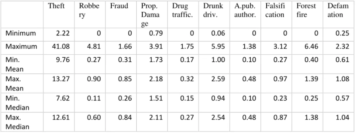
In this section basic descriptive statistics were calculated for each table. Mean, median, standard deviation, sample variance, kurtosis, skewness, range, maximal and minimal values, were calculated for each variable in each data table. The results are provided in the annex. Summary statistics for the set of 19 tables is shown in the table 2. The results show that crime rate of crimes related to Theft was significantly highest during the whole period. Both mean and median values of variable Theft were significantly highest during the whole period. Observing the range of mean and median values, it is possible conclude that after variable Theft, the highest crime rates were related with variables Property damage and Drunk Driving during the study period. Other crimes types have generally significantly lower crime rates. It is notable that maximal and minimal mean values are higher than maximal and minimal median values for all variables.
Theft Robbe
ry Fraud Prop. Dama ge
Drug
traffic. Drunk driv. A.pub. author. Falsification Forest fire Defamation
Minimum 2.22 0 0 0.79 0 0.06 0 0 0 0.25
Maximum 41.08 4.81 1.66 3.91 1.75 5.95 1.38 3.12 6.46 2.32
Min. Mean
9.76 0.27 0.31 1.73 0.17 1.00 0.10 0.27 0.40 0.61
Max. Mean
13.27 0.90 0.85 2.18 0.32 2.59 0.48 0.97 1.39 1.08
Min. Median
7.62 0.11 0.26 1.51 0.15 0.94 0.10 0.23 0.25 0.57
Max. Median
12.61 0.60 0.84 2.11 0.27 2.54 0.48 0.87 1.38 1.04
24
5. Results and discussion
The spatial analysis of crime evolution in Portugal will be done in two steps. In the first step global analysis will be done in order to extract information about general trends in crime evolution in Portugal between 1995 and 2013. In the second step spatial analysis of crime evolution between 1995 and 2013 will be done. The first analysis will enable us compare local trend with global trends and to have a clearer picture how crimes evolved in Portugal.
5.1. Global analysis
5.1.1. Crime evolution in Portugal
Crime evolution in Portugal between 1995 and 2013 will be analysed using principal component analysis. Years of period 1995-2013 are considered as observations, while different crime types are considered as variables. Crimes are measured in crime rates. Principal component analysis enables us to represent crime evolution in a lower dimension space.
Since variable Theft (without violence) has significantly higher crime rates than any other variable (especially compared to Homicide and Corruption) we decided to work with metric on the observation space 𝑀1/𝑠2.
25
Figure 3 Percentage of inertia explained by each component
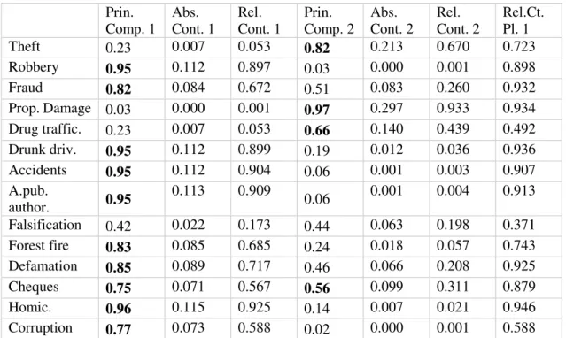
The interpretation of two components can be obtained by calculating their correlation with variables under study. Correlation of variables with components is shown in the Table 3. Since we decided to use standardized data, the image representing correlation of the variables with principal components is the exact projection of standardized variables on the plane generated by first two principal components. Correlation of variables with components and their position on the plane generated by 1st two principal components is shown on the Figure 4.
Prin.
Comp. 1 Abs. Cont. 1 Rel. Cont. 1 Prin. Comp. 2 Abs. Cont. 2 Rel. Cont. 2 Rel.Ct. Pl. 1
Theft 0.23 0.007 0.053 0.82 0.213 0.670 0.723
Robbery 0.95 0.112 0.897 0.03 0.000 0.001 0.898
Fraud 0.82 0.084 0.672 0.51 0.083 0.260 0.932
Prop. Damage 0.03 0.000 0.001 0.97 0.297 0.933 0.934
Drug traffic. 0.23 0.007 0.053 0.66 0.140 0.439 0.492
Drunk driv. 0.95 0.112 0.899 0.19 0.012 0.036 0.936
Accidents 0.95 0.112 0.904 0.06 0.001 0.003 0.907
A.pub.
author. 0.95 0.113 0.909 0.06 0.001 0.004 0.913
Falsification 0.42 0.022 0.173 0.44 0.063 0.198 0.371
Forest fire 0.83 0.085 0.685 0.24 0.018 0.057 0.743
Defamation 0.85 0.089 0.717 0.46 0.066 0.208 0.925
Cheques 0.75 0.071 0.567 0.56 0.099 0.311 0.879
Homic. 0.96 0.115 0.925 0.14 0.007 0.021 0.946
Corruption 0.77 0.073 0.588 0.02 0.000 0.001 0.588
Table 3 Absolute and relative contributions of variables on the 1st plane
0.00 10.00 20.00 30.00 40.00 50.00 60.00 70.00
1 2 3 4 5 6 7 8 9 10 11 12 13 14
In
e
rti
a (
in
%
)
26
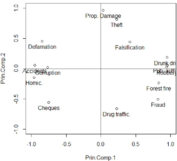
Figure 4 Correlation of the variables with principal components
Absolute and relative contributions of variables are shown in Table 3. It is notable that
variable Falsification crimes doesn’t have a good representation on the 1st plane. Variables
Drug trafficking and Corruption also don’t have a good representation on the 1st plane like other variable. However, it is still possible to interpret their general evolution. Other variables have good or even excellent representation on the 1st plane. Absolute contribution shows that 1st axis explains variables Robbery, Fraud, Crimes against public authority, Drunk driving, Forest fire crimes, Issuing cheques without provision, Corruption, Homicide, Homicides and offences to physical integrity due to traffic accidents, and Defamation. 2nd axis explains variables Theft, Property damage, Drug trafficking, but also Fraud and Issuing cheques without provision which have lower contribution.
27
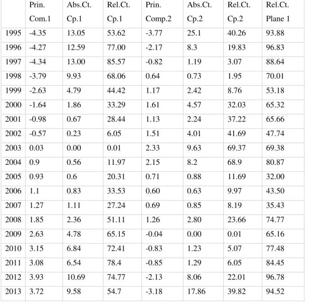
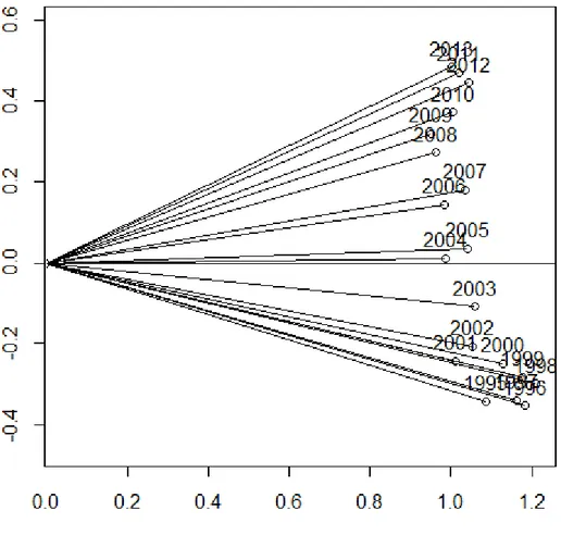
possible not only to represent years in 1st principal plane, but also to draw a trajectory of observations (Figure 5). It is notable that the years 1999, 2002, 2006 and especially years 2005
and 2007 don’t have a good a representation on the 1st principal plane. Relative contributions also show that years of the first and third period have especially good representation on the 1st principal plane. It is also notable that the years 1999-2009 have a lower contribution to 1st axis. Years at the beginning (1995-1998) and at the end (2008-2013) of the period have a high absolute contribution to the 1st axis. Years 1995 and 2013 have the significantly highest absolute contribution to 2nd axis. However years 1996, 1999-2004, and 2012 also have a high absolute contribution to 2nd axis.
Prin.
Com.1
Abs.Ct. Cp.1
Rel.Ct. Cp.1
Prin. Comp.2
Abs.Ct. Cp.2
Rel.Ct. Cp.2
Rel.Ct. Plane 1
1995 -4.35 13.05 53.62 -3.77 25.1 40.26 93.88
1996 -4.27 12.59 77.00 -2.17 8.3 19.83 96.83
1997 -4.34 13.00 85.57 -0.82 1.19 3.07 88.64
1998 -3.79 9.93 68.06 0.64 0.73 1.95 70.01
1999 -2.63 4.79 44.42 1.17 2.42 8.76 53.18
2000 -1.64 1.86 33.29 1.61 4.57 32.03 65.32
2001 -0.98 0.67 28.44 1.13 2.24 37.22 65.66
2002 -0.57 0.23 6.05 1.51 4.01 41.69 47.74
2003 0.03 0.00 0.01 2.33 9.63 69.37 69.38
2004 0.9 0.56 11.97 2.15 8.2 68.9 80.87
2005 0.93 0.6 20.31 0.71 0.88 11.69 32.00
2006 1.1 0.83 33.53 0.60 0.63 9.97 43.50
2007 1.27 1.11 27.24 0.69 0.85 8.19 35.43
2008 1.85 2.36 51.11 1.26 2.80 23.66 74.77
2009 2.63 4.78 65.15 -0.04 0.00 0.01 65.16
2010 3.15 6.84 72.41 -0.83 1.23 5.07 77.48
2011 3.08 6.54 78.4 -0.85 1.29 6.05 84.45
2012 3.93 10.69 74.77 -2.13 8.06 22.01 96.78
2013 3.72 9.58 54.7 -3.18 17.86 39.82 94.52
28
In the context of our analysis this trajectory on the Figure 5 represents crime evolution in Portugal. In order to interpret crime evolution it is important to interpret the axes first.
1st PC opposes the years with the higher crime rates of crimes like Robbery (with violence), Fraud, Crimes against public authority, Drunk driving, Forest fire crimes and lower crime rates of crimes like Issuing cheques without provision, Corruption, Homicide, Homicides and offences to physical integrity due to traffic accidents, Defamation on one side, and years with the lower crime rates of crimes like Robbery (with violence), Fraud, Crimes against public authority, Drunk driving, Forest fire crimes and higher crime rates of crimes like Issuing cheques without provision, Corruption, Homicide, Homicides and offences to physical integrity due to traffic accidents, Defamation.
2nd PC opposes the years with the higher crime rates of crimes like Property damage and Theft (without violence) and lower crime rates of crimes like Drug trafficking, Fraud and Issuing cheques without provision on one side, and years with the lower crime rates of crimes like Property damage and Theft (without violence) and higher crime rates of crimes like Drug trafficking, Fraud and Issuing cheques without provision on the other side. It is notable that variables like Property damage and Theft (without violence) have much higher absolute correlation value then the variables Drug trafficking, Fraud and Issuing cheques without provision.
Falsification crimes have a positive correlation with both components, but they don’t
have a good representation on the 1st principal plane; these crimes are not interpretable on the 1st principal plane.
29
Figure 5 Crime evolution represented on the 1st principal plane
Years between 1995 and 1998 form the first period. These years are characterized by relatively high crime rates of Issuing cheques without provision, Corruption, Homicide, Homicides and offences to physical integrity due to traffic accidents, Defamation and relatively low crime rates of crimes like Robbery (with violence), Fraud, Crimes against public authority, Drunk driving, Forest fire crimes. While the values of these crimes were relatively constant, this period was characterized by a very rapid increase of crime rates of Property damage and Theft (without violence) and general decrease of Drug trafficking crimes. It is also interesting to note that crime rates of Issuing cheques without provision were also decreasing, but they still remained relatively high during the whole period. Crime rates of crime Defamation were slightly increasing towards the end of the period.
30
generally low crime rates of Drug trafficking crimes. Crime rates of Property damage and Theft were slowly increasing until 2003, when they reached their maximum. After 2003 they were decreasing slowly. However, this period was characterized by constant and rapid diminution of crime rates of Issuing cheques without provision, Corruption, Homicide, Homicides and offences to physical integrity due to traffic accidents, and Defamation and a constant and rapid increase of crime rates of crimes like Robbery (with violence), Fraud, Crimes against public authority, Drunk driving, and Forest fire crimes. Inside this period years 2005, 2006, and 2007 show specific crime dynamics, but we have to take into account that quality of their representation on the 1st principal plane is not good.
The last period is formed by years between 2008 and 2013. It is characterized by low crime rates of Issuing cheques without provision, Corruption, Homicide, Homicides and offences to physical integrity due to traffic accidents, and Defamation. Crime rates of these crimes generally have continued to decrease generally, but in this period very slowly. This period is also characterized by high crime rates of Robbery (with violence), Fraud, Crimes against public authority, Drunk driving, Forest fire crimes. Crime rates of these crimes have continued to increase generally, but in this period very slowly with the exception of Forest fire crimes and Fraud. Crime rates of Forest fire crimes and especially Fraud have continued to increase significantly in the last years. This period is especially characterized by a significant and constant diminution of crime rates of Property damage and Theft (without violence) and increase of crime rates of Drug trafficking.
Finally, it is possible to conclude that changes in crime rates off various crimes were gradual and they have followed few general patterns. Only crime rates of Falsification crimes
don’t show gradual changes; they even don’t seem to follow any rule.
Generally crime rates of crimes like Issuing cheques without provision, Corruption, Homicide, Homicides and offences to physical integrity due to traffic accidents, and Defamation have significantly decreased in the period 1995-2013. Decrease of crime rates of these crimes has started after 1998, with the exception of crime Issuing cheques without provision, which crime rates show constant decrease during the whole period 1995-2013. Defamation has shown an increase of crime rates in the period 1995-1998. It is important to note that crime evolution of Corruption crimes is not explained so well on the 1st principal plane.
31
Forest fire crimes and especially Fraud whose crime rates have continued to increase rapidly in the years after 2008.
Crimes like Drug trafficking, Theft and Property damage have shown circular evolution. Crime rates of Theft and Property damage were increasing until 2003 (with the fast increase in the period 1995-1998). After 2003 their crime rates have been decreasing. In 2013 their crime rates were in the similar level like in 1995. Crime rates of Drug trafficking crimes were high at the beginning of the period, they were relatively low in the middle of the period, and finally they were high at the end of the period.
Proximity of the variables on the 1st principal plane enables us to identify few groups of crimes with similar crime evolution patterns. First group includes Homicide, Homicides and offences to physical integrity due to traffic accidents, and Corruption. Second group includes Theft and Property damage. Third group includes Robbery, Crimes against public authority, and Drunk driving.
It is possible to observe an interesting phenomena; crimes with similar evolutions
generally don’t belong to same crime types. It seems that different socio-economic factors and public policies have resulted in similar crime evolution patterns. Also sometimes crime evolution patterns are unexpected. For example, while the number of Drunk driving crimes has significantly increased, the number of Homicides and offences to physical integrity due to traffic accidents has decreased. Also Theft and Robbery don’t follow the same evolution
pattern; Theft is correlated with Property damage, while Robbery is correlated with Drunk driving.
In the further studies it may be interesting to analyse socio-economic factors and public policies which affected crime evolution. It may be interesting to analyse why changes have occurred in years 1998 and 2008, especially having in mind the beginning of the recession in Portugal in 2008.
5.1.2. Interstructure analysis of data tables
The second part of the global crime analysis is going to be to detect similarity and to observe is there a commune structure in 19 data tables with 10 variables and 30 observations where each table represents one year of the 1995-2013 period. This will be done using STATIS technique - finding the interstructure. This procedure will indicate if it is going to be possible to obtain a good compromise.
32
First part of interstructure analysis find RV coefficients for different years. RV coefficients represent the correlation between spatial crime structures in different years and are shown in the annex. They have the same order of size and they are always greater than 0.67. It can be concluded that crime structures in all the years of the studied period are correlated.
Norms of data tables are shown in the table annex. It is notable that norms have relatively similar values, which indicates that it may be possible to obtain a good compromise without normalizing the objects Wt.
Non-centred Euclidian image of interstructure is obtained by performing a PCA on the matrix of Hilbert-Schmind scalar products S (annex) and is shown on the Figure 6. Eigenvalues of a matrix S, together with the percentage of inertia associated to each of them is shown in the table X- annex. Inertia related with the 1st axis is about 81.23%, while inertia related with 2nd axis is about 6.57%. Since first principal plane captures about 87.8% of inertia, interstructure is well represented. Each year is represented in the form of OM line segment where O is the centre of the coordinate system and M a point on the plane.
33
It is notable that in general the pairs of years which have lower values of RV coefficients (the ones that have bigger angles between their line segments on the Figure 6) are the ones that are more far away in the time period, while the ones with higher RV coefficients (the ones that have smaller angles between their line segments on the image) are the ones that are more far away in the time period. Since RV coefficients represent correlations between crime structures in different years, it can concluded that crime structures in neighbouring years were very correlated and as the years passed the correlation was lower and lower. There wasn't any dramatic change in the crime evolution between years; the change in the crime patterns was graduate.
Since RV coefficients and norms have the same order of size, the compromise will represents a good overview of the data structure.
5.2. Spatial analysis of crime evolution in Portugal
5.2.1. Definition of the compromise
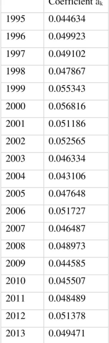
Compromise matrix was calculated as the linear combination of intrastructurte matrices. Eigenvectors of the compromise matrix are shown in the table X-annex. Eigenvalues of a matrix W, together with the percentage of inertia associated to each of them is shown in the annex.
34
Coefficient ak
1995 0.044634
1996 0.049923
1997 0.049102
1998 0.047867
1999 0.055343
2000 0.056816
2001 0.051186
2002 0.052565
2003 0.046334
2004 0.043106
2005 0.047648
2006 0.051727
2007 0.046487
2008 0.048973
2009 0.044585
2010 0.045507
2011 0.048489
2012 0.051378
2013 0.049471
Table 5 Coefficients ak associated with Wk matrices represented by years
Diagonalization of matrix WD showed that 1st principal component explains about 43.93% of inertia, while 2nd principal component explains about 14.15 % of inertia. The decision was to represent compromise with two principal components; 1st principal plane explains about 58.07 % of inertia.
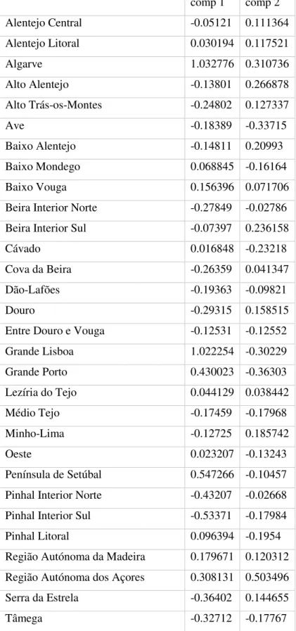
5.2.2. Interpretation of compromise
35
Correlation of variables with the 1st and 2nd principal component is shown in the annex. Trajectories of correlations of the variables with principal components are also shown in annex.
Variables Theft (without violence), Robbery (with violence), Fraud, Drug trafficking, Falsification crimes show a strong correlation with 1st PC during the whole period, while the variable Forest fire crimes shows a strong to moderate negative correlation with 1st PC during the whole period. Very strong positive correlation is especially notable for the variable Theft (without violence), which is a crime type with the significantly highest crime rate in Portugal. These variables do not show a significant correlation with 2nd PC. However it is notable that variable Robbery (with violence) has a low but stable positive correlation with 2nd PC, while variable Drug trafficking has a low but constant negative correlation with 2nd PC.
Variable Drunk driving has a medium positive correlation with the 2nd PC at the beginning of the study period and high positive correlation with the 2nd PC in rest of the period. It has a very low positive correlation with 1st PC.
Variable Property damage has a medium to low positive correlation with the 2nd PC at the beginning of the period, while at the end of the period the correlation becomes higher. It is notable that the correlation with the 1st PC is high and positive only in the period 1996-2002.
Variable Crimes against public authority are strong positive correlation with the 1st PC at the beginning (1995-2000) and at the end (2007-2013) of the study period. It is interesting to note that the correlation with the 2nd PC was medium positive in the period 2001-2008 when the correlation with 1st PC is low.
Variable Defamation has a stable medium positive correlation with the 2nd PC, while the correlation with the 1st PC evolves gradually from being medium positive at the beginning of the study period, then it becomes almost insignificant in the middle of the period, and finally it becomes moderate negative at the end of the period.
In general 1st PC opposes regions with higher crime rates related with crimes like Theft (without violence), Robbery (with violence), Fraud, Drug trafficking, Falsification and lower crime rates related with Forest fire crimes on one side, and regions with lower crime rates related with crimes like Theft (without violence), Robbery (with violence), Fraud, Drug trafficking, Falsification and higher crime rates related with Forest fire crimes on the other side during the whole period 1995-2013.