Infrared and millimetre-wave scintillometry in the suburban environment – Part 1: Structure parameters

www.atmos-meas-tech.net/8/1385/2015/ doi:10.5194/amt-8-1385-2015

© Author(s) 2015. CC Attribution 3.0 License.

Infrared and millimetre-wave scintillometry in the suburban

environment – Part 1: Structure parameters

H. C. Ward1,2,3, J. G. Evans1, C. S. B. Grimmond2,3, and J. Bradford4

1_{Centre for Ecology and Hydrology, Wallingford, Oxfordshire, OX10 8BB, UK} 2_{Department of Geography, King’s College London, London, WC2R 2LS, UK} 3_{Department of Meteorology, University of Reading, Reading, RG6 6BB, UK}

4_{Space Science Department, Rutherford Appleton Laboratory, Didcot, Oxfordshire, OX11 0QX, UK} Correspondence to:H. C. Ward (h.c.ward@reading.ac.uk)

Received: 3 October 2014 – Published in Atmos. Meas. Tech. Discuss.: 17 November 2014 Revised: 10 February 2015 – Accepted: 28 February 2015 – Published: 20 March 2015

Abstract. Scintillometry, a form of ground-based remote sensing, provides the capability to estimate surface heat fluxes over scales of a few hundred metres to kilometres. Measurements are spatial averages, making this technique particularly valuable over areas with moderate heterogene-ity such as mixed agricultural or urban environments. In this study, we present the structure parameters of temperature and humidity, which can be related to the sensible and la-tent heat fluxes through similarity theory, for a suburban area in the UK. The fluxes are provided in the second paper of this two-part series. A millimetre-wave scintillometer was combined with an infrared scintillometer along a 5.5 km path over northern Swindon. The pairing of these two wavelengths offers sensitivity to both temperature and humidity fluctua-tions, and the correlation between wavelengths is also used to retrieve the path-averaged temperature–humidity correla-tion. Comparison is made with structure parameters calcu-lated from an eddy covariance station located close to the centre of the scintillometer path. The performance of the measurement techniques under different conditions is dis-cussed. Similar behaviour is seen between the two data sets at sub-daily timescales. For the two summer-to-winter periods presented here, similar evolution is displayed across the sea-sons. A higher vegetation fraction within the scintillometer source area is consistent with the lower Bowen ratio observed (midday Bowen ratio <1) compared with more built-up ar-eas around the eddy covariance station. The energy partition-ing is further explored in the companion paper.

1 Introduction

Scintillometer measurements have been carried out at sites of varying complexity, from tests of the technique under simple conditions (Hill and Ochs, 1978; De Bruin et al., 1993) to studies investigating the complications of non-ideal terrain, including heterogeneous land cover (Beyrich et al., 2002; Meijninger et al., 2002a, 2006; Ezzahar et al., 2007) and complex topography (Poggio et al., 2000; Evans, 2009; Evans et al., 2012). On the whole, these studies have shown that scintillometers installed above or close to the blending height can provide valuable area-averaged fluxes.

With careful selection of a suitable path, the scintillometry technique has been successfully used in urban areas. Kanda et al. (2002), the first to obtain the sensible heat flux in an ur-ban setting, used two small aperture scintillometers installed at different heights on a 250 m path over a dense residential area of Tokyo. Other small aperture studies include measure-ments in Basel (Roth et al., 2006) and London (Pauscher, 2010). Large aperture scintillometers are increasingly being used over longer urban paths (Lagouarde et al., 2006; Gou-vea and Grimmond, 2010; Mestayer et al., 2011; Wood et al., 2013; Zieli´nski et al., 2013). These infrared (or optical) scin-tillometers must rely on the residual of the energy balance if the latent heat flux is to be estimated. However, the com-plexity of the energy balance (Oke, 1987) means this is usu-ally not attempted in urban areas. In particular the significant storage heat flux (Offerle et al., 2005) and contribution from anthropogenic activities (Klysik, 1996; Allen et al., 2011) are both very difficult to measure.

Sensitivity to both humidity and temperature fluctuations can be achieved with a two-wavelength scintillometer sys-tem. In this case, the structure parameter of humidity can be obtained in addition to the structure parameter of tem-perature, from which both the sensible heat flux (QH) and

latent heat flux (QE) can be found (Hill et al., 1988; An-dreas, 1989). Several studies have reported successful esti-mates ofQE using the two-wavelength method (Meijninger et al. 2002a, 2006; Evans, 2009; Evans et al., 2010). This technique requires that a value of the temperature–humidity correlation coefficient,rT q, be assumed. OftenrT qis taken to be±1, indicating perfect correlation, as in Green et al. (2001) and Meijninger et al. (2002a), but other values have also been used: Kohsiek and Herben (1983) used rT q=0.87; Evans (2009) used rT q=0.8; and Meijninger et al. (2006) used measured rT q from a nearby EC station with val-ues between₋0.5 and 0.9. Previous studies measuringrT q with fast-response sensors suggest daytime values tend to be smaller than 1, typically around 0.8. For example: 0.75 at a flat, homogeneous site (Kohsiek, 1982); 0.76 over sandy soil with patchy vegetation (Andreas et al., 1998); 0.70– 0.95 for unstable conditions over heterogeneous farmland (Meijninger et al., 2002a). Nocturnal values of rT q down to−1 are rarely seen (Andreas et al., 1998; Beyrich et al., 2005; Meijninger et al., 2006).

Some studies have suggested thatrT qvaries with stability (Li et al., 2011; Nordbo et al., 2013), although others have

shown no clear relation (De Bruin et al., 1993; Roth, 1993). Explanation of_|rT q| 6=1 is often related to surface hetero-geneity (Roth, 1993; Andreas et al., 1998; Lüdi et al., 2005) but low values have been obtained over homogeneous sur-faces too (Kohsiek, 1982; De Bruin et al. 1993). In almost all previous studies, measurements ofrT q were made using point sensors.

Lüdi et al. (2005) outlined a method to obtain path-averaged values ofrT q using a two-wavelength scintillome-ter system. This “bichromatic-correlation” method is an ex-tension of the two-wavelength technique and involves cor-relating the signals from each scintillometer, thus enabling determination of the combined temperature–humidity fluctu-ations andrT q. The bichromatic-correlation method, applied for the first time during the LITFASS-2003 campaign, gave promising results (Beyrich et al., 2005; Lüdi et al., 2005). An overview of the second study, during LITFASS-2009, is given in Beyrich et al. (2012).

Aside from enabling more accurate structure parameters and fluxes to be obtained from scintillometry, improved knowledge of rT q has wider applications. Correlations be-tween scalars are thought to be useful indicators for the vi-olation of Monin–Obukhov similarity theory (MOST) (Hill, 1989; Andreas et al., 1998). Correlations are also relevant to the understanding and modelling of turbulent transport pro-cesses through physical quantities such as eddy diffusivities. The objectives of this research are to measure structure parameters and obtain large-area sensible and latent heat fluxes for a suburban area. In this two-part study, a 94 GHz millimetre-wave scintillometer was deployed alongside an infrared scintillometer over the town of Swindon, UK. This is the first use of such a system in the urban environment. In Part 1, structure parameters from the two-wavelength system are compared to structure parameters calculated from an EC system and measured values ofrT q are discussed. In Part 2 (Ward et al., 2015), the sensible and latent heat fluxes are determined and analysed. These spatially integrated obser-vations represent the behaviour of the suburban surface over an area of 5–10 km2and constitute by far the longest data set (14 months) that uses these techniques. The performance of the techniques is assessed under a range of conditions, and their strengths and weaknesses are examined. This paper of-fers insight into the behaviour of the structure parameters and rT q at various timescales (daily, seasonal and inter-annual), including how they respond to energy and water availability, surface cover and changing meteorological conditions.

2 Theory

C_y2₌[y(x+δ)−y(x)]

2

δ2/3 , (1)

whereδis the spatial separation between two points andy(x) is the value of the variable at locationx. The cross-structure parameter between two variables is defined analogously; for example the cross-structure parameter between temperature, T, and specific humidity,q, is written as follows:

CT q=[

T (x₊δ)₋T (x)_][q(x₊δ)₋q(x)_]

δ2/3 . (2)

2.1 Obtaining structure parameters from scintillometry

The refractive index structure parameter (Cn2) is fundamental to scintillometry. For each wavelength, λ, it can be written (Hill et al., 1980) as follows:

C_n2₌A

2 T T2C

2 T +2

ATAq T q CT q+

A2_q

q2C 2

q, (3)

where C_T2 is the structure parameter of temperature, C2_q the structure parameter of specific humidity, CT q the temperature–humidity cross-structure parameter andAT and Aq are the structure parameter coefficients for tempera-ture and specific humidity, respectively, given in Ward et al. (2013b) as At and Aq (see their Table 2). These coef-ficients contain the wavelength dependence of C_n2, whereas C_T2,C_q2andCT q are properties of the atmosphere. EachC2n measurement is made up of a combination of the three un-knowns:C_T2,C_q2andCT q.

AsC_n2from large aperture optical or near-infrared scintil-lometers is almost entirely made up of temperature fluctua-tions (C_T2), the (usually small) contributions fromCT q and C_q2can be approximated using the Bowen ratio,β (Wesely, 1976; Moene, 2003):

C_n2_≈A

2 T T2C

2 T

1+Aq q

T AT

cp

Lv

β−1

2

≈A

2 T T2C

2 T

1₊0.03β−12, (4)

wherecpis the specific heat capacity of air at constant

pres-sure,Lvis the latent heat of vaporisation and the value 0.03

is for typical atmospheric conditions (T₌300 K, pressure (p)₌105Pa). The required Bowen ratio may be found by us-ing the available energy as an input to the iteration to obtain the sensible heat flux (e.g. Green and Hayashi, 1998; Mei-jninger et al., 2002b; Solignac et al., 2009). Calculation of the latent heat flux must rely on the energy balance (Ezzahar et al., 2009; Guyot et al., 2009; Evans et al., 2012; Samain et al., 2012b). This is the single-wavelength scintillometry method.

As demonstrated by Hill et al. (1988) and Andreas (1989), a two-wavelength scintillometer system enables retrieval of

bothC_T2andC_q2via simultaneous equations (Eq. (3) for each wavelength). The two-wavelength method has the significant advantage of providing both sensible and latent heat fluxes without resorting to the energy balance, but a value for the temperature–humidity correlation coefficientrT qmust be as-sumed in the substitutionCT q=rT q(CT2Cq2)1/2.

The bichromatic-correlation method uses the same combi-nation of optical and millimetre wavelength scintillometers as for the two-wavelength method, but additionally exploits the correlation between optical and millimetre-wave signals to obtain a third equation for the cross-structure parameter, Cn1n2(Lüdi et al. 2005):

Cn1n2=

AT1AT2

T2 C 2 T+

_A

T1Aq2+AT2Aq1

T q

CT q

+Aq_q1A2q2C 2

q, (5)

where the subscripts 1 and 2 refer to the different wave-lengths. In this study, λ1 denotes optical (specifically

880_×10−9_{m) and λ}

2 millimetre (3.2×10−3m)

wave-lengths. Thus all three unknown meteorological structure pa-rameters (C2_T,C_q2andCT q) can be found from the three mea-sured refractive index structure parameters by inverting the matrix equation (Lüdi et al., 2005):

(Cn1n1Cn2n2Cn1n2)=M





C_T2 CT q

C2_q



, (6)

where the inverse matrixM−1is given by

M−1₌ T

2_q2

AT1Aq2−AT2Aq1

2 ×     

A2_q2 q2

A2_q1 q2

−2Aq1Aq2

q2

−AT2Aq2

T q

−AT1Aq1

T q

(AT1Aq2+AT2Aq1)

T q A2_T2

T2

A2_T1

T2 −

2AT1AT2

T2      . (7)

As mentioned above, the structure parameter coefficientsAT andAqshould be those formulated using specific humidity.

For the bichromatic-correlation method, the value ofCT q can therefore be used to effectively measure the temperature– humidity correlation coefficient:

rT q= CT q

q

C_T2C2 q

. (8)

If MOST assumptions (i.e.T₋qsimilarity) are satisfied, the Bowen ratio can be calculated from the structure parameters (Andreas, 1990; Lüdi et al., 2005)

β₌sgnCT q

cp

Lv

s

C_T2

C2 q

. (9)

C2_T=A

2

q2Cn1n1+Aq21Cn2n2+2rT qAq1Aq2S2λ√Cn1n1Cn2n2

AT1Aq2−AT2Aq1

2

T−2 , (10a)

C2_q=A

2

T2Cn1n1+A2T1Cn2n2+2rT qAT1AT2S2λ

√

Cn1n1Cn2n2

AT1Aq2−AT2Aq1

2

q−2 , (10b)

whereS2λis±1. This choice of sign is an inherent ambiguity of the two-wavelength method and represents two possible solutions toCn2n2(Hill et al., 1988; Hill, 1997). For lowβ,

when humidity fluctuations dominate Cn2n2thenS2λ= +1, whereasS2λ= −1 is required at largerβ. The sign ofS2λis not known a priori but must be assumed. Often the two solu-tions forβ indicate which is the most likely solution for the atmospheric conditions and site characteristics (Hill, 1997). When expressed as a function ofβ, a minimum inCn2n2is

revealed due to the coefficientsAT andAqhaving opposite signs at millimetre wavelengths. The contribution ofCT qto Cn2n2(middle term in Eq. 3) is negative whenCT q>0, so for moderateβ the terms in Equation 3 can cancel out leav-ingCn2n2close to zero (Hill et al., 1988; Otto et al., 1996). In

practice, zeroCn2n2will not be observed because the

instru-ment has a finite noise floor (andrT q6=1). Instead the scin-tillation signal may be close to, or below, the detection limit of the instrument, resulting in reduced sensitivity around the region of minimumCn2n2 and a tendency for the derivedβ

to be biased away from (below, forS2λ= +1) the value at which minimumCn2n2occurs. The problematic region is

ex-pected to occur forβ_≈2–3 (Leijnse et al., 2007; Ward et al., 2013b).

2.2 Obtaining structure parameters from eddy covariance

Conversion between spatial and temporal domains enables calculation of structure parameters from point measure-ments, such as those from EC instrumentation. The spatial structure function,Dyy_x, can be written (e.g. Stull, 1988) as follows:

Dyy_x(δ)= [y(x+δ)−y(x)]2. (11) Analogously the temporal structure function,Dyy_t, is given by

Dyy_t(τ )= [y(t+τ )−y(t )]2, (12) whereτis the temporal separation andy(t )is the value of the variable at time t. Bosveld (1999) gives the conversion be-tween temporal and spatial structure functions using the hor-izontal wind vector, U_{, and the variances of the three wind} components,σ_u,v,w2 :

Dyy_x(δ)=

Dyy_t(δ/U)

1−19 σ2

u

U2 +

1 3

σ2

v

U2 +

1 3

σ2

w

U2

. (13)

Thus temporal structure functions (Eq. 12) can be calcu-lated from EC measurements, converted to spatial struc-ture functions (Eq. 13) and then strucstruc-ture parameters

Figure 1.Aerial photograph (2009, GeoPerspectives©) of the study area showing the locations of the two-wavelength scintillometer path (BLS–MWS), eddy covariance station (EC) and two mete-orological stations (METsub, METroof). The location of Swindon within the British Isles is shown (top right panel).

(Cy2=Dyy_x(δ) δ−2/3 defines Cy2 for δ in the inertial sub-range). Unlike fluxes, structure parameters are strongly height dependent.

3 Experimental details

3.1 Instrumental setup and site description

Table 1.The instrumental setup. For the scintillometers the mean height of the beam above the land surface (zm) is given (for the effective measurement height (zef) see Table 2); for METroofthe heights above the roof surface are given. Roughness length,z0, and displacement height,zd, were not calculated for the rooftop site. Tx denotes transmitter, Rx receiver.

Instrumentation Height[m] Location Path z0 zd

length _[m_{] [}m_]

[m]

Two-wavelength 44.3 51◦36′33.9′′N 1◦47′38.6′′W (Tx) 5492 0.7 4.9 scintillometer system 51◦33′38.1′′N 1◦46′55.3′′W (Rx)

EC station 12.5 51◦35′4.6′′N 1◦47′53.2′′W – 0.5 3.5

METsub 10.6 (WXT) 51◦35′4.6′′N 1◦47′53.2′′W – 0.5 3.5 10.1 (NR01)

METroof 2.0 (WXT) 51◦34′0.3′′N 1◦47′5.3′′W – – – 1.1 (NR01)

Bedford, UK) near the base of the mast. These were located in the garden of a residential property approximately 3 km north of the town centre, where the surrounding land use is predominantly residential, consisting of 1–2 storey houses with gardens. Full details are given in Ward et al. (2013a). In addition to the meteorological instrumentation at the EC site (METsub), a second weather station was established on the

rooftop of a modern office building close to the town centre (METroof). The setup is summarised in Table 1. To provide

a combined data set of continuous input variables required for scintillometry processing,T, RH,pandUfrom METroof

were linearly adjusted to gap-fill METsub(required for<1 %

ofT, RH andpand<2 % ofU data), based on regressions with concurrent data from METsub(9 May 2011–31

Decem-ber 2012).

Northern Swindon is typical of suburban areas in the UK. The area has a relatively large proportion of vegetation and there is a large nature reserve just north of the centre of the study area, which lies directly underneath the scintillome-ter path. The town centre at the south of the study area has the highest density of buildings and roads (Fig. 1). Indus-trial areas to the east and southwest with little vegetation contribute to measurement source areas under stable condi-tions (see Part 2). Despite the variety of land-cover types, many neighbourhoods appear fairly homogeneous at a scale of a few hundred metres. The area shown in Fig. 1 has land cover that is 14 % buildings, 31 % impervious, 53 % vegeta-tion, 1 % water and 2 % pervious. Land cover, topography and building and tree heights were derived from a spatial database for Swindon (5 m resolution, see Ward et al. (2013a) for more information).

To obtain representative measurements it is important to be high enough above the surface that quantities are sufficiently well-blended (i.e. high enough that turbulent mixing aver-ages out the influence of surface heterogeneity), although recent studies have shown successful use of scintillometers even below the blending height (Meijninger et al., 2002b;

Ez-zahar et al., 2007). Based on the average height of the rough-ness elements (i.e. buildings and trees) the blending height is estimated at about 15–30 m for the BLS–MWS source area (Pasquill, 1974; Garratt, 1978). The scintillometer trans-mitters, mounted on custom-built brackets, were installed at 28 m a.g.l. on a television transmitter mast. The receivers of the BLS–MWS system were mounted at 26 m a.g.l. on a rooftop in Swindon town centre. The resulting path is slanted (Fig. 2).

The effective heights of the scintillometers are given in Table 2, calculated according to the stability independent ap-proximation (Eq. (15) of Hartogensis et al., 2003). These es-timates include adjustment to account for the curvature of the earth and displacement height,zd (Table 1). Displacement

heights were calculated from the mean height of the rough-ness elements, zH, within a distance of ±1000 m

perpen-dicular to the scintillometer path (and+500 m in the direc-tion parallel to the path), using the rule-of-thumbzd=0.7zH

(Garratt, 1992; Grimmond and Oke, 1999). In the case of the EC station, zH was calculated within 500 m of the EC

mast. The difference in BLS and MWS path-weighting func-tions (Fig. 3) means that the BLS, MWS and combined BLS– MWS covariance measurements are representative of differ-ent heights even though the BLS and MWS beams essdiffer-entially traverse the same path (Evans and De Bruin, 2011).

Table 2.Instrument and site-dependent characteristics of the scintillometers and paired scintillometer system.

Instrument characteristics Site-dependent characteristics

Scintillometer Wavelength Aperture Fresnel Effective Scaling (S)

[m_] diameter zone height factor

[m] [m] [m]

BLS (C_n1n1) 880_×10−9 0.145 – 45.0 –

MWS (Cn2n2) 3.2×10−3 0.25 4 42.8 0.952

BLS–MWS (C_n1n2) – – – 43.1 0.958

Figure 2.Cross-section of the land surface (metres above sea level) and height of obstacles (buildings and trees) along the BLS–MWS path. Tx denotes transmitter, Rx receiver.

Figure 3.Path-weighting functions for the infrared scintillometer (BLS disk), the MWS and the BLS–MWS combination, normalised so that the total area under each curve equals one.

The data presented here are for the complete months when the BLS–MWS system was functioning: July– December 2011 and May–December 2012. From Jan-uary 2012 to April 2012 the MWS was not operational due to a fault.

3.2 Data collection, processing and quality control 3.2.1 Scintillometry

In this study, Cn1n1 is used to denote the refractive index

structure parameter from the BLS, to distinguish fromCn2n2

(MWS) andCn1n2(BLS–MWS cross term). The BLS900 is

a dual-beam scintillometer with two transmitter disks (only one disk is used here for combination with the MWS). The signal intensity of each BLS disk was sampled and stored at 500 Hz (raw data) and statistics including the mean and standard deviation of signal intensity were provided at 30 s intervals by the Scintec software (SRun v1-07). Addition-ally, the signal intensities of both BLS disks and of the MWS were sampled at 100 Hz by a CR5000 datalogger (Campbell Scientific Ltd., Loughborough, UK). These data were pro-cessed using code written in R (The R Foundation for Statis-tical Computing). Data were subjected to initial quality con-trol involving the removal of dropouts (when the BLS makes a background measurement) and despiking. The BLS and MWS signals were bandpass filtered to remove contributions below 0.06 Hz and above 20 Hz for the calculation ofCn2n2

andCn1n2. The low-frequency cut-off reduces the influence

of absorption fluctuations. At 10 min intervals, the variances, covariance and mean values of the signals were calculated, from which the log-amplitude variances (σ_χ2₁,σ_χ2₂) and co-variance (σχ1χ2) were obtained (Tatarski, 1961). To

con-vert between the log-amplitude (co)variances and refractive index (cross-)structure parameters the following equations were used:

Cn1n1=4.48D7/3L−3σχ21, (14a)

Cn1n2=8.93k−7/6L−11/6σχ1χ2, (14c)

whereDrefers to the aperture diameter of the infrared scin-tillometer, kto the wave number (2π/λ) of the millimetre-wave scintillometer andLto the path length (Tables 1 and 2). These equations can be derived from the full forms of the log-amplitude (co)variances, which express the path weighting of the instrument, the aperture averaging by the finite size of transmitter and receiver, the turbulence spectrum (assumed to be the Kolmogorov spectrum, e.g. Monin and Yaglom, 1971) and the separation of the beams if applicable (Eqs. A1 and A2, Appendix A). Note that Eq. (14c) is specific to the setup described here (beam separation, path length and in-strument characteristics) and could be expressed in terms of D rather thank. Equation (14b) was obtained using the full formula (Eq. A2) instead of the small aperture approxima-tion (in which the Bessel funcapproxima-tions accounting for aperture averaging are excluded) and is also specific to this setup. The approximation can result in an inaccuracy even for long paths (Appendix A). Equation (14a) for the infrared scintillometer is a standard result and was first demonstrated by Wang et al. (1978).

Quality-control procedures rejected data during periods of low signal strength (usually caused by rain or fog). BLS data were rejected when the received signal intensity dropped be-low 0.5 of the daily maximum value. For the MWS a thresh-old of 0.33 of the daily maximum intensity was used, and MWS data were also removed when the BLS signal intensity was below the 0.5 threshold indicating obscuration along the BLS–MWS path. The data points directly adjacent to those failing the signal strength checks were also removed. Rain was recorded at the EC site for 10 % of the data set and fog often occurred, particularly during autumn and winter morn-ings (based on observations during site visits). Values ofC2_n outside reasonable thresholds were excluded (nineCn1n1

val-ues and one Cn1n2 value). The resulting data available for

analysis constitute 79 % of the total possible 10 min values (N=61 776).

Kleissl et al. (2010) suggest an empirical threshold for the onset of saturation for infrared large aperture scintil-lometers of Cn1n1>0.074D5/3λ1/3L−8/3. Approximately

21 % of the BLS data were above this threshold of 3.2×10−15m−2/3. BLS data were corrected for saturation using a look-up table of numerical values based on the mod-ulation transfer function of Clifford et al. (1974). The cor-rection increasedCn1n1by around 5 % overall (∼10 %

dur-ing summer daytimes). Where the estimated correction was larger than 25 %, data were removed instead (46 values in to-tal). MWS data were well below the saturation threshold of 5.0×10−11m−2/3(Clifford et al., 1974) and were not cor-rected. The BLS–MWS covariance was not corrected as a methodology is yet to be determined (Beyrich et al., 2012). There is therefore increased uncertainty in these measure-ments due to the extent of currently applicable theory.

To use the refractive index structure parameters in Eq. (6) (or Eq. 10a–b),Cn1n1,Cn2n2andCn1n2must be

representa-tive of the same height. TheSfactors (Evans and De Bruin, 2011) given in Table 2 were applied toCn2n2from the MWS

andCn1n2 from the BLS–MWS to scale them to the same

effective height asCn1n1 from the BLS. These factors

ac-count for the difference in effective heights between the three C_n2measurements resulting from the combination of different weighting functions and changing beam elevation along the path (Sect. 3.1). TheSfactors are relatively close to unity as the height differences are reasonably small for this setup. The approximation of using stability independentS factors was made here (incorporating stability would give values ranging from 1.0 under very stable conditions to 0.9 for free convec-tion). Calculation of the meteorological structure parameters proceeds as described in Sect. 2.

Data were processed using each of the three techniques in order to investigate their respective merits, although the focus is on the two-wavelength and bichromatic-correlation methods. No Bowen ratio correction was applied for the single-wavelength method (Eq. 4), given the uncertainties in estimating the available energy in urban environments. The impact is estimated to be a 6 % overestimation in C_T2 (based on β from the two-wavelength method). The posi-tions of twice-daily minima inCn1n1 were used to indicate

stability transitions (Samain et al., 2012a) and assign posi-tive or negaposi-tiverT q for the two-wavelength method. For the two-wavelength method rT q= ±0.8 was assumed and the solution corresponding toS2λ= +1 was chosen. To distin-guish between the methods applied (single-wavelength, two-wavelength, bichromatic-correlation), the subscripts “1λ”, “2λ” and “bc” are used.

3.2.2 Eddy covariance

Structure parameters were also derived from 20 Hz raw EC data. Sonic and IRGA data were time aligned by seek-ing maximum covariance between variables. Initial quality control incorporated threshold checks, outlier detection and despiking. A fixed temporal separation of τ₌1 s was de-cided upon after investigation into suitable values in the in-ertial subrange. Calculation ofC_T2,C2_qandCT q included the Schotanus et al. (1983) correction for sonic temperature as discussed in Braam (2008) and Braam et al. (2012). No cor-rections were made for spectral losses caused by the spa-tial separation of the sonic and IRGA and their finite path lengths, which can be expected to result in underestimations of about 5–7 % (Hill, 1991; Hartogensis et al., 2002).

Figure 4. Example power spectral density (PSD) and frequency (f) spectra for(a, b)the BLS and (c, d)unfiltered MWS for 14:30– 15:00 UTC on 2 July 2011. Smoothed spectra (data divided into 100 bins) are shown in black. The dashed lines represent theoretically predicted slopes of−12/3 and−8/3 for the BLS and MWS, respectively.

To facilitate comparison between EC and scintillometer data sets, the EC structure parameters were scaled to match the height of the scintillometer data using MOST functions (with the constants suggested by Andreas (1988) and assum-ing identical height scalassum-ing of temperature and humidity, see Eq. 3a and b in Part 2).

Since the source areas are different between EC and BLS– MWS systems, the structure parameters obtained are not ex-pected to be in perfect agreement. The BLS–MWS footprint is generally more vegetated than the EC footprint (56 % ver-sus 44 %). However, comparisons are useful for a number of reasons. As EC is a widely used technique, it permits evaluation of the scintillometer system to a certain extent, through comparison of trends and patterns of behaviour even if absolute values differ. Both systems have merits and lim-itations: scintillometers are spatially representative; EC is a more direct measurement but (open-path IRGAs) cannot pro-vide data after rainfall and there are issues with energy clo-sure (Foken, 2008). Analysis of both approaches can there-fore provide a more complete picture of the environment studied.

4 Instrument performance

An unidentified instrumental noise problem affecting the CEH-RAL MWS has been reported elsewhere (Van Kesteren, 2008; Evans, 2009; Beyrich et al., 2012). Fol-lowing extensive testing, the cause of the issue was finally established and the instrument repaired in June 2011. The spectra obtained are now close to the ideal shapes predicted by theory and suggest good instrument performance with a low noise floor (Fig. 4). An upper estimate for the MWS noise limit isCn2n2∼1×10−15m−2/3. The observed noise

limit of the BLS is of the order ofCn1n1∼5×10−17m−2/3

in agreement with the manufacturer’s specification (Scintec, 2009).

5 Results and discussion 5.1 Structure parameters

5.1.1 Refractive index structure parameters

The refractive index structure parameters measured by the BLS (Cn1n1) and MWS (Cn2n2) and the cross-structure

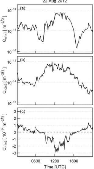
parameter from the covariance of the BLS–MWS signals (Cn1n2) follow clear diurnal cycles. Data for an example day

are plotted in Fig. 5. WhilstCn1n1andCn2n2remain positive,

the cross-structure parameter can be positive or negative de-pending on whether the infrared and millimetre-wave signals are correlated or anti-correlated.Cn1n2 tends to be negative

during the day and positive at night. The sign change oc-curs at the morning and evening stability transitions. Typ-ically Cn1n1 passes through sharp minima at these times,

whereas the diurnal course of Cn2n2 is flatter and wider,

without clearly defined minima. These findings are in broad agreement with data from the LITFASS campaigns (Beyrich et al., 2005, 2012; Lüdi et al., 2005).

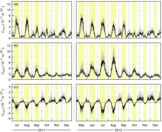
When averaged by month (Fig. 6), the diurnal patterns are enhanced and seasonal trends are revealed. The amplitudes of the diurnal cycles are largest in summer, except Cn1n1

which peaks slightly earlier in the year.Cn1n1is closely

re-lated to C_T2 and, in turn, the sensible heat flux. Hence the peak inCn1n1in late spring reflects the annual cycle ofQH:

approaching maximum insolation in mid-summer, the total energy input is large but evapotranspiration rates are lim-ited by phenological development as maximal leaf area is not reached until later in the year. During winter, low radiative in-put means the midday maximum inCn1n1is small; larger

val-ues are observed at night. For millimetre wavelengths,Cn2n2

tends to remain low throughout the night. The diurnal cy-cle inCn1n2is maintained across all months with changes in

the position of the zero crossings determined mainly by at-mospheric stability (usually the sign ofQH, related to

avail-able energy and day length). In December Cn1n2 is

en-Figure 5.Structure parameters of the refractive index as measured by(a)the BLS and(b)the MWS, and(c)the cross-structure param-eter as measured by the BLS–MWS combination for an example day (22 August 2012).

ergy input decreases from summer to winter. Using the po-sitions of Cn1n1 minima to indicate the stability transition

times generally worked well for this data set, although per-formance was poorer in winter when stability changes tend to be less well defined and conditions may remain close to neutral throughout the day. Following the method described in Samain et al. (2012a), additional restrictions were imposed on the times of morning (here after 04:00 UTC) and evening (before 21:00 UTC) transitions. In a few cases, cumulative daily net radiation was also used to distinguish Cn1n1

min-ima that were due to sudden cloud cover during daytime from Cn1n1minima that were due to a change of stability.

5.1.2 Meteorological structure parameters

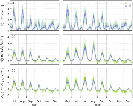
There are clear parallels between the refractive index struc-ture parameters (Fig. 6) and the meteorological strucstruc-ture pa-rameters (Fig. 7). Cn1n1 is dominated by C_T2 with a small

contribution fromCT q (of about 5 %, which decreases asβ increases; Green et al., 2001). The cross-structure parame-terCn1n2consists mostly of theCT qterm and a contribution fromC_T2. WhenCn1n2is negativeCT qis positive. The dom-inant term inCn2n2depends on the Bowen ratio:Cq2usually dominates at lowβ, but theCT q term is also important and forms a negative contribution toCn2n2during daytime (when

CT qis positive).

5.1.3 Comparison of eddy covariance and scintillometry techniques

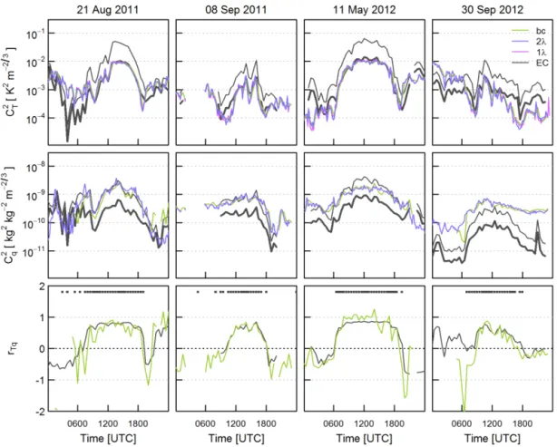
In Fig. 8, meteorological structure parameters for individ-ual days are compared to EC. As structure parameters are strongly height dependent, the EC values have been scaled to match the height of the scintillometry results (zef=45.0 m,

Sect. 3.2.2). Scintillometer and EC values ofC_T2 andC_q2are not expected to agree exactly due to the differences in source area and land-cover composition; however, these indepen-dent measurements are often remarkably consistent. The cor-relation between the scintillometer and EC data sets gives confidence that the scintillometer setup is responding reason-ably to changes in boundary layer conditions and measuring within the surface layer. The square of the correlation coef-ficient (r2) between the two-wavelength scintillometry and height-scaled EC data is 0.72 and 0.60 forC_T2 andC_q2, re-spectively. Considering daytime only,r2increases to 0.86 for C_T2, but remains about the same forC_q2at 0.56.

These results suggest βEC is larger than βBLS–MWS, but

the fact that the estimates ofC_T2 are closely matched while C_q2_{_BLS–MWS} is larger than C_q2_{_EC} is indicative of a more complex situation (see Part 2).

Structure parameters from the BLS–MWS and EC sys-tems exhibit the same trends (but have different magnitudes) over the course of the year (Fig. 9).C_T2 is largest during late spring, whilstC_q2peaks in July and August. There is variabil-ity between years attributed to drier conditions in 2011 than 2012 (July–August rainfall was 110 mm in 2011, 184 mm in 2012). In July–August 2011,C_T2 was larger andC_q2smaller than in the same months in 2012. In general, 2012 was much wetter than 2011, which explains consistently lower β in 2012 (Fig. 9c). The BLS–MWS gives lower β com-pared to EC (during summer daytimeβBLS–MWS≈0.5 and

βEC≈1.0), which is in accordance with the BLS–MWS

foot-print being more vegetated, but similar seasonal behaviour is seen. In winter β becomes negative as a result of reduced radiative input, and the difference between βBLS–MWS and

βECdecreases. In terms of fluxes, evapotranspiration

contin-ues throughout winter because moisture is readily available, whereas energy is limited soQHis directed towards the

Figure 6.Median diurnal cycles and inter-quartile ranges (grey shading) of the structure parameters of the refractive index as measured by(a)the BLS and(b)the MWS, and(c)the cross-structure parameter as measured by the BLS–MWS combination, separated by month. Yellow shading indicates periods whenQ∗>0 W m−2.

could be inferred from the diurnal course ofrT q(Fig. 10) and positions ofCn1n1minima (Fig. 6a).

The performance of EC and scintillometry differs with at-mospheric conditions. EC data from open-path gas analysers cannot be used if the instrument windows are wet, such as during and after rainfall (Heusinkveld et al., 2008). Conse-quently, water vapour measurements from open-path systems significantly under-represent these times and may result in an appreciable underestimation of mean QE (Ramamurthy

and Bou-Zeid, 2014) and C_q2. Mean values for C_T2 calcu-lated using daytime data only when all quantities are avail-able concurrently (i.e.C_T2 andC_q2from EC, two-wavelength and bichromatic-correlation methods – grey bars, Fig. 9) are larger compared to mean values calculated using all available daytime data (coloured bars) due to the exclusion of periods during and directly following rain (whenC_T2 is typically rel-atively low QE is relatively high). In September 2012 the

opposite effect is seen because the EC data were limited by dirty IRGA windows when the weather was dry and sunny; hence it is generally highC_T2values that are eliminated in this case. During summer, monthly meanC_q2_{_BLS–MWS}is reduced slightly for the concurrent data set (grey bars) as times of highQEwhen water and energy are plentiful have been

ex-cluded. The overall results are not substantially changed for the restricted subset:C_T2_{_BLS–MWS}andC_T2_{_EC} are still simi-lar, whilstC_q2_{_BLS–MWS}still exceedsC_q2_{_EC}, although the

dif-ference betweenC_q2_{_BLS–MWS}andC_q2_{_EC}is reduced slightly. The spectral correction (Sect. 3.3.2) would increase the EC structure parameters by 5–7 %, which would further reduce the discrepancy between EC and BLS–MWS values.

As for most previous two-wavelength campaigns, typical Bowen ratios for this path are expected to lie below the prob-lematic region of minimumCn2n2 (Sect. 2.1). Other urban

studies suggest daytime β of around 1.0–1.5 for suburban sites, lower when precipitation is frequent (Grimmond and Oke, 1995) and strongly dependent on the amount of vege-tation (Grimmond and Oke, 2002; Christen and Vogt, 2004). However, although averageβ remains below 1.5 (Fig. 9c), changing surface conditions can drive down the evapotran-spiration on the timescale of a few days (e.g. drying of im-pervious surfaces; Ward et al., 2013a, or at agricultural sites, senescing crops; Evans et al., 2012), producing substantial excursions from the average β. Such excursions are seen in this data set, particularly for βEC, whereas β2λ seems to be limited to values ≤ 1.3. There are two potential is-sues here: (a) the two-wavelength sign ambiguity and (b) the region of reduced sensitivity around the Cn2n2 minimum

(Sect. 2.1). Selecting S2λ= +1 automatically restricts β2λ to values below that at which the terms in Equation 3 can-cel out (β2λ_min=2.0–2.6 for this data set). For a few cases

Figure 7.Median diurnal cycles and inter-quartile ranges (shading) of the meteorological structure parameters(a)C_T2,(b)C_q2and(c)CT q calculated using the bichromatic (bc) and two-wavelength (2λ) techniques. In (c) CT q for the two-wavelength technique is given by

±0.8 (C_T2C_q2)1/2.

bichromatic-correlation results to identify times of high β suggests the impact is small (βbc> β2λ_min for a very small

proportion of the data (<0.3 % of daytime values)). A more significant issue appears to be reduced measurement capabil-ity forβ2λ>1.3. As the trueβ increases, ifCn2n2does not

decrease as much as expected from theory,β2λwill likely be underestimated, and the corresponding C_q2 (andQE) could

be overestimated. It is thought that noise in the setup (instru-mental or unwanted intensity fluctuations from absorption, for example) may constrain the measured value of β2λ to a greater extent than suggested in the literature.

This region of reduced sensitivity of Cn2n2also

compro-mises the performance of the bichromatic method, as mea-sured Cn2n2 will be mostly made up of noise contributions

relative to the near-zero true value of Cn2n2. It follows that

the correlation between BLS and MWS signals in this region is expected to be dominated by common instrumental or at-mospheric effects such as absorption, or any electrical inter-ference, mounting vibrations or obscuration along the path. Although these effects were not found to be problematic gen-erally, they could become significant when the refraction sig-nal diminishes at moderateβ.

5.1.4 Comparison of two-wavelength and bichromatic-correlation methods

The three estimates of C2_T for the BLS–MWS path are similar (on average within 6 %) whether the bichromatic-correlation, two-wavelength or single-wavelength approach is used. Larger deviations are seen betweenC_q2_{_bc}andC_q2_{_2λ} when measuredrT q_bcdiffers from the value assumed (±0.8)

in the two-wavelength method (e.g. 21 August 2011, Fig. 8). During daytime,C_q2_{_2λ} is slightly larger thanC_q2_{_bc} in 2011 but the opposite is true for most of 2012 (Figs. 7b and 9b). This could be due to higher values of rT q_bc in 2012 (see

Fig. 10), which result in smaller C_T2 but larger C_q2 when rT q>0. The value ofrT q has a greater impact on Cq2than C_T2 (compare error bars in Fig. 9a and b). HadrT q_2λ been assumed to be_±1.0 instead of_±0.8,C_q2_{_2λ}would have been 7 % higher andC_T2_{_2λ}1 % lower.

During winter night-times, large differences are observed betweenC_q2_{_bc}andC_q2_{_2λ}which cannot be explained by dif-ferences inrT q. Negative values ofC_q2_{_bc}are frequently ob-tained (Fig. 7b). These do not have a physical interpreta-tion but are indicative of measurement limitainterpreta-tions and co-incide with large negativeCT q_bc, which results from large

positiveCn1n2(i.e. high correlation between BLS and MWS

Figure 8.Structure parameters of temperature and humidity and the temperature–humidity correlation coefficient for selected days, derived from eddy covariance measurements (EC) and from the BLS–MWS system using the single-wavelength (1λ), two-wavelength (2λ) and bichromatic-correlation (bc) methods. EC structure parameters are shown for the EC measurement height (thin line) and scaled to the effective height of the scintillometry results (thick line). Unstable times according to the EC data (LOb<0) are indicated by grey dots. Single-wavelength and two-wavelength data are for 10 min intervals; EC and bichromatic-correlation data are for 30 min intervals.

the bichromatic-correlation data show much greater variabil-ity than the two-wavelength data. To reduce this variabilvariabil-ity, bichromatic-correlation data are presented as 30 min aver-ages (except in Fig. 7).

5.2 Temperature–humidity correlation

MeasuredrT q_bcfollows similar seasonal and diurnal trends

torT q_EC(Fig. 10). During summer, there is a clear plateau

of around 0.8 during daytime and the transition times when rT q changes sign are of short duration compared to the day length. In winter rT q remains below zero for most of the day but peaks at positive values around midday, though the average midday rT q is less than 1. The EC data rarely ex-ceed the range −0.75 to 0.85, whereas inspection of the time-series reveals thatrT q_bc almost always follows a

typ-ical diurnal course but individual points may vary about the general trend (e.g. Fig. 8). Some unrealistic values of |rT q_bc|>1 are observed, even when averaged to 30 min

(Figs. 8 and 10). Lüdi et al. (2005) also reported frequent occurrences of |rT q_bc|>1. SincerT q is a correlation

coef-ficient, these values (>1) do not have a physical interpreta-tion, but result from uncertainties and thus indicate limita-tions of the measurement. The uncertainty inCn1n2is around

20 % at best (Lüdi et al., 2005). This inherent uncertainty as-sociated with individual measurements means the structure parameters from the bichromatic-correlation method show greater variability than from the two-wavelength method (Sect. 5.1.4), particularlyC_q2andCT q which have a greater dependence onCn1n2thanC_T2 does. For this reason,

bichro-matic results are presented at 30 min, rather than 10 min as for the two-wavelength method (Figs. 8–11). In addition, to calculate rT q, the structure parameters must be combined (Eq. 8) and sorT q amasses the uncertainties in each of the measurements.

Figure 9.Mean daytime (incoming shortwave radiationK_↓>5 W m−2)(a, b)structure parameters and(c)Bowen ratio calculated according to Eq. (9) for each month calculated for the BLS–MWS system (bichromatic-correlation and two-wavelength approaches) and eddy covari-ance data scaled to match the BLS–MWS height. For the two-wavelength resultsrT q_2λ= ±0.8; error bars in(a)and(b)indicate the effect of assumingr_{T q}values of_±0.5 and_±1.0. Light grey bars(a, b)indicate means calculated when bothC_T2 andC_q2from all three methods (bc, 2λand EC) are available.

Figure 10.Monthly median diurnal cycles and inter-quartile ranges (shading) of the temperature–humidity correlation coefficient calculated from the BLS–MWS system via the bichromatic-correlation method and from EC.

smaller magnitude at night (Kohsiek, 1982; Andreas et al., 1998; Meijninger et al., 2002a; Beyrich et al., 2005). Ac-cording to Lüdi et al. (2005) theT₋q anti-correlation ob-served at night is “less pronounced” than the positive correla-tion during daytime; Meijninger et al. (2006) also foundrT q ranged between₋0.5 and 0.9. Our measurements conducted in the suburban environment do not indicate lowerT₋q cor-relation than over other surfaces. Indeed, it is thought that rT q_EC likely underestimates the true values (as the sonic

and IRGA are spatially separated). This supports the use of

MOST, and gives confidence that the measurements are made at sufficient height that the effects of surface heterogeneity are well-blended. Furthermore, the two-wavelength assump-tionrT q= +0.8 is seen to be reasonable for unstable condi-tions, although probablyrT q= −0.8 is too large during sta-ble conditions. Figure 10 suggests that these assumptions are less justified in winter.

In Fig. 11 values ofrT q measured in this study are sepa-rated into unstable and stable conditions (based onLObfrom

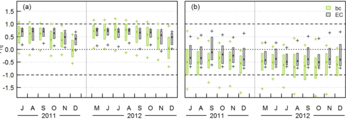
Figure 11.Box plots ofr_{T q}from eddy covariance (EC) and the BLS–MWS bichromatic-correlation method for(a)unstable and(b)stable conditions. Crosses indicate the 10th and 90th percentiles, boxes enclose the inter-quartile range (25th to 75th percentiles) and heavy lines indicate the medians.

Cn1n1 for the scintillometer data). During unstable

condi-tions, measuredrT qis positive and around 0.6 to 0.9, whereas the stable values tend to be smaller at around−0.3 to−0.5 and more variable. In winterrT qis smaller and more variable (medianrT q_ECdecreases from>0.7 in summer to<0.5 in

December for unstable conditions). Some studies have indi-cated a dependence of temperature–humidity correlation on LOb, with larger deviations from MOST as neutral

condi-tions are approached (Li et al., 2011; Nordbo et al., 2013), although other studies differ (De Bruin et al., 1993; Roth, 1993). Part 2 further explores the scaling of temperature and humidity structure parameters with stability.

Some instances of positive nocturnal rT q are observed when the fluxes have the same signs, i.e. either unsta-ble (QH>0) conditions prevail, or (more frequently)

dew-fall (QE<0) is observed under stable conditions (as on 21 August 2011 after 21:30 UTC, Fig. 8). In these cases the two-wavelength method is limited as negativerT q must be assumed in the absence of other information, whereas the bichromatic-correlation method often captures this be-haviour. In general, nocturnal structure parameters (and fluxes) tend to be small so the absolute errors introduced by rT q_2λof the wrong sign are fairly small, though they will al-ways be biased in the same direction and so will accumulate over time.

The bichromatic-correlation data suggest larger daytime rT q in 2012 compared to 2011, but this is not seen in the EC data. The contrast between patches of hot, dry impervi-ous areas and cool, wet vegetation may be reduced by alto-gether wetter surfaces in 2012, which is thought to increase correlation between temperature and humidity (Lamaud and Irvine, 2006; Moene and Schüttemeyer, 2008; Ramamurthy and Bou-Zeid, 2014). On the other hand, Lüdi et al. (2005) found lower rT q coincides with lower β. Experiments de-signed to investigate the behaviour of rT q (and the perfor-mance of the bichromatic-correlation technique) under dif-ferent conditions would be beneficial.

In winter, and also during night-time, turbulence tends to be less well-developed. This presents challenges to measure-ment theory. Measuremeasure-ments are also more likely to be out-side the surface layer when stable stratification occurs and the boundary layer height is smaller. Due to the rough sur-face, near-neutral conditions were far more common than stable and, for the most part, there remains a close match between the diurnal behaviour of EC and scintillometer mea-surements. On the few occasions when strongly stable condi-tions were observed at the EC station, a comparison of time series indicated periods when the BLS–MWS was possibly above the surface layer and thus potentially affected by other processes not related to surface fluxes. However, these were relatively rare occurrences.

In this study, the performance of the bichromatic-correlation method was generally observed to be poor under conditions of low crosswind speeds (the wind speed com-ponent perpendicular to the BLS–MWS path). At times of low or near-zero crosswinds (<2 m s−1), the retrieved quan-tities are less robust,|rT q_bc|>1 is commonly observed and

rT q_bcis highly variable frequently changing sign (even

dur-ing the day when both turbulent fluxes are reasonably ex-pected to be positive and EC data do not suggest otherwise). The reason for this is unknown, but two possible explana-tions are considered here. Firstly, Taylor’s frozen turbulence hypothesis is assumed in order to relate intensity fluctuations toC_n2 (Clifford, 1971; Wang et al., 1981). When crosswind speeds are low, this assumption is less justified and eddies de-cay as they are slowly blown through the beam. Correlation between the received scintillation pattern from one sample to the next is reduced compared to higher crosswind cases (Poggio et al., 2000). Correlation between the scintillation signals of the BLS and MWS will likely show greater varia-tion too, depending on how the decay of eddies affects each beam, which would result in variability inCn1n2that

prop-agates through torT q_bc. Secondly, when wind speeds are

events cause spuriously high correlation between BLS and MWS signals which outweighs the correlated scintillation signal the technique aims to measure. Given the complex-ity of this suburban site it is difficult to draw firm conclu-sions on this apparent effect of crosswind on bichromatic scintillometry at this stage. Given that the position of the spectrum is known to change with wind speed (Medeiros Filho et al., 1983; Nieveen et al., 1998; Ward et al., 2011), and thatC_n2can be underestimated if the filter excludes part of the scintillation signal under very low wind speed condi-tions (Solignac et al., 2012), the suitability of the bandpass filter was also re-examined. However, the choice of filter fre-quency did not seem to explain the poor performance and modifying the filter frequencies did not resolve the issues. Small changes in filter frequency generally did not produce substantial changes to the results, suggesting that the fre-quencies chosen are suitable for this data set, but it is not critical that those exact values are used.

6 Conclusions

This study reports the first use of a two-wavelength scin-tillometer system in an urban area. The behaviour of struc-ture parameters and temperastruc-ture–humidity correlation is in-vestigated at various timescales. By examining the structure parameters themselves, more direct insight into the perfor-mance of the measurement techniques is gained; assessment of fluxes introduces additional uncertainties (e.g. similarity functions). Furthermore, structure parameters are important quantities in their own right. The spatial and temporal reso-lution of scintillometry observations offers advantages for as-similation into, or evaluation of, hydro-meteorological mod-els. One approach for achieving this would be to work with structure parameters directly, rather than fluxes (e.g. Wood et al., 2013).

The structure parameters presented here extend previous observations to a different climatic region, different land-cover type and, most importantly, across a much longer time period. Summertime behaviour is broadly in agreement with other published trials (Beyrich et al., 2005; Lüdi et al., 2005) but the long time-series presented here offers insight into seasonal variations. Day length, or more specifically, atmo-spheric stability, has a distinctive impact on the diurnal cycle of structure parameters andrT q. Overall, the structure param-eters obtained from the BLS–MWS and EC systems exhibit remarkably similar tendencies. The Bowen ratio calculated from the measured structure parameters decreases across the two summer-to-winter periods studied here, andβBLS–MWS

is smaller thanβEC, attributed partly to different source area

characteristics but also probable differences between the ob-servational techniques. Part 2 explores energy partitioning further via turbulent fluxes.

As well as extending the two-wavelength technique to a new environment, several recently developed improvements

have been implemented in the processing. To obtain the structure parameter of refractive index from the millimetre-wave scintillometer, the validity of the small aperture ap-proximation is considered and the more accurate full for-mula used instead. To adjust for the difference in effective heights between the BLS and MWS, theSfactor approach of Evans and De Bruin (2011) was used. The structure param-eters use the specific humidity formulation outlined in Ward et al. (2013b). The cross-correlation between BLS and MWS signals enabled estimation of the temperature–humidity cor-relation coefficient, thus extending the application of the bichromatic-correlation method to the suburban surface.

The bichromatic-correlation method sometimes returns values outside the physically meaningful range |rT q| ≤1. The inherent variability of the cross-structure parameter Cn1n2 limits the accuracy of any particular measurement,

whereas the two-wavelength results are more robust over shorter periods. On average, results closely follow the ex-pected diurnal cycle of correlated temperature and humid-ity during the day and anti-correlated at night. MeasuredrT q is approximately 0.6–0.9 in unstable conditions; stable val-ues are more variable but tend to be smaller in magnitude, averaging around−0.3 to−0.5. ObservedrT q was furthest from±1 during winter and in near-neutral conditions. Sim-ilar behaviour is seen inrT q_bc andrT q_EC, including times

when the assumed two-wavelength value will be wrong. Two-wavelength scintillometer systems have considerable potential to deliver large-area measurements representative of complex environments. Limitations of the two-wavelength method include the ambiguity due to two possible solutions forβ and the region of reduced sensitivity around theCn2n2

minimum. Research is needed; firstly, to better understand the behaviour in this region and secondly, to investigate im-provements to the instrumentation, setup or post-processing to minimise the impact. Advantages of the bichromatic-correlation method include additional information about the atmospheric conditions (e.g. the relative sign of the heat fluxes and to what extent MOST conditions are satisfied). For the minimal extra hardware requirements, the recommenda-tion is therefore to measure the bichromatic correlarecommenda-tion even if the additional information is not used directly in data pro-cessing.

Appendix A: Validity of the small aperture approximation for millimetre-wave scintillometers The log amplitude of a scintillometer system can be written in a generalised form (e.g. Lüdi et al., 2005),

σχ1χ2=4π2k1k20.033C2n

∞ Z

0

dK

L

Z

0

dxKK−11/3

×sin

K2x(L−x) 2k1L

sin

K2x(L−x) 2k2L

× _2J

1(0.5KDr1x/L)

0.5KDr1x/L

2J1(0.5KDt1(1−x/L))

0.5KDt1(1−x/L)

×

2J1(0.5KDr2x/L)

0.5KDr2x/L

2J1(0.5KDt2(1−x/L))

0.5KDt2(1−x/L)

J0(K|d|), (A1)

whereσχ1χ2 is the covariance of log amplitude,Cn2the re-fractive index structure parameter,Kthe eddy wave number andx the position along the path of lengthL; kis the op-tical wave number, d the beam separation, andDthe aper-ture diameter of the receiver (subscript r) or transmitter (sub-script t) for each instrument (sub(sub-script 1 or 2).J0andJ1are

Bessel functions of the first kind. The three-dimensional Kol-mogorov spectrum8n(K)=0.033Cn2K−11/3is assumed.

For a single instrument, this reduces to the standard for-mula for a large aperture scintillometer (Hill and Ochs, 1978):

σ_χ2₌4π2k20.033C_n2

∞

Z

0

dK L

Z

0

dxKK−11/3

×sin2

K2x(L₋x) 2kL

×

2J1(0.5KDrx/L)

0.5KDrx/L

2

×

2J1(0.5KDt(1−x/L))

0.5KDt(1−x/L)

2

. (A2)

For cases when aperture averaging is unimportant, the stan-dard formula for small aperture scintillometers,

σ_χ2₌4π2k20.033Cn2 ∞

Z

0

dK L

Z

0

dxKK−11/3

×sin2

_K2_x(L

−x) 2kL

, (A3)

gives

σ_χ2₌ck7/6L11/6C_n2 (A4) on integration withc₌0.124 (Meijninger et al., 2002a, 2006; Lüdi et al., 2005).

Here we consider the validity of applying the small aper-ture approximation to millimetre-wave, microwave and ra-diowave systems. For the effects of aperture averaging to be insignificant, the aperture diameter must be sufficiently small compared to the maximal diameter of the first Fresnel zone, F₌(λL)1/2_{. WithF around 10 timesD, the small aperture}

Acknowledgements. We would like to thank Alan Warwick and Cyril Barrett for constructing the scintillometer mounting brackets, Geoff Wicks for assisting with the electronics and the residents of Swindon, who very kindly gave permission for equipment to be installed on their property. We are grateful to Wim Kohsiek and Oscar Hartogensis for their helpful discussions regarding the work presented in Appendix A. This work was funded by the Natural Environment Research Council, UK.

Edited by: F. S. Marzano

References

Allen, L., Lindberg, F., and Grimmond, C. S. B.: Global to city scale urban anthropogenic heat flux: model and variability, Int. J. Cli-matol., 31, 1990–2005, doi:10.1002/joc.2210, 2011.

Andreas, E. L.: Estimating C2_nover snow and sea ice from meteo-rological data, J. Opt. Soc. Am., 5, 481–495, 1988.

Andreas, E. L.: Two-wavelength method of measuring path-averaged turbulent surface heat fluxes, J. Atmos. Ocean. Tech., 6, 280–292, 1989.

Andreas, E. L.: Three-wavelength method of measuring path-averaged turbulent heat fluxes, J. Atmos. Ocean. Tech., 7, 801– 814, 1990.

Andreas, E. L., Hill, R. J., Gosz, J. R., Moore, D. I., Otto, W. D., and Sarma, A. D.: Statistics of surface-layer turbulence over terrain with metre-scale heterogeneity, Bound.-Lay. Meteorol., 86, 379– 408, 1998.

Beyrich, F., De Bruin, H. A. R., Meijninger, W. M. L., Schipper, J. W., and Lohse, H.: Results from one-year continuous opera-tion of a large aperture scintillometer over a heterogeneous land surface, Bound.-Lay. Meteorol., 105, 85–97, 2002.

Beyrich, F., Kouznetsov, R. D., Leps, J. P., Lüdi, A., Mei-jninger, W. M. L., and Weisensee, U.: Structure parameters for temperature and humidity from simultaneous eddy-covariance and scintillometer measurements, Meteorol. Z., 14, 641–649, doi:10.1127/0941-2948/2005/0064, 2005.

Beyrich, F., Bange, J., Hartogensis, O., Raasch, S., Braam, M., van Dinther, D., Gräf, D., van Kesteren, B., van den Kroonenberg, A., Maronga, B., Martin, S., and Moene, A.: Towards a Validation of Scintillometer Measurements: The LITFASS-2009 Experiment, Bound.-Lay. Meteorol., 144, 83–112, doi:10.1007/s10546-012-9715-8, 2012.

Bosveld, F. C.: The KNMI Garderen experiment: micro-meteorological observations 1988–1989, KNMI, the Nether-lands, 57 pp., 1999.

Braam, M.: Determination of the surface sensible heat flux from the structure parameter of temperature at 60 m height during day-time, KNMI, the Netherlands, 42 pp., 2008.

Braam, M., Bosveld, F., and Moene, A.: On Monin–Obukhov Scal-ing in and Above the Atmospheric Surface Layer: The Complex-ities of Elevated Scintillometer Measurements, Bound.-Lay. Me-teorol., 144, 157–177, doi:10.1007/s10546-012-9716-7, 2012. Christen, A. and Vogt, R.: Energy and radiation balance of

a central European city, Int. J. Climatol., 24, 1395–1421, doi:10.1002/joc.1074, 2004.

Clifford, S. F.: Temporal-frequency spectra for a spherical wave propagating through atmospheric turbulence, J. Opt. Soc. Am., 61, 1285–1292, 1971.

Clifford, S. F., Ochs, G. R., and Lawrence, R. S.: Saturation of opti-cal scintillation by strong turbulence, J. Opt. Soc. Am., 64, 148– 154, 1974.

De Bruin, H. A. R., Kohsiek, W., and Van den Hurk, B. J. J. M.: A verification of some methods to determine the fluxes of momentum, sensible heat, and water-vapour using standard-deviation and structure parameter of scalar meteorological quan-tities, Bound.-Lay. Meteorol. 63, 231–257, 1993.

Evans, J. G.: Long-Path Scintillometry over Complex Terrain to Determine Areal-Averaged Sensible and Latent Heat Fluxes, PhD Thesis, Soil Science Department, the University of Read-ing, ReadRead-ing, UK, 181 pp., 2009.

Evans, J. G. and De Bruin, H. A. R.: The Effective Height of a Two-Wavelength Scintillometer System, Bound.-Lay. Meteorol., 141, 165–177, doi:10.1007/s10546-011-9634-0, 2011.

Evans, J. G., McNeil, D. D., Finch, J. F., Murray, T., Harding, R. J., and Verhoef, A.: Evaporation Measurements at Kilometre Scales Determined Using Two-wavelength Scintillometry. BHS Third International Symposium, Role of Hydrology in Managing Con-sequences of a Changing Global Environment Newcastle Univer-sity, 19–23 July 2010, Newcastle upon Tyne, UK, 2010. Evans, J. G., McNeil, D. D., Finch, J. W., Murray, T., Harding,

R. J., Ward, H. C., and Verhoef, A.: Determination of turbulent heat fluxes using a large aperture scintillometer over undulating mixed agricultural terrain, Agr. Forest Meteorol., 166–167, 221– 233, 2012.

Ezzahar, J., Chehbouni, A., and Hoedjes, J. C. B.: On the applica-tion of scintillometry over heterogeneous grids, J. Hydrol., 334, 493–501, doi:10.1016/j.jhydrol.2006.10.027, 2007.

Ezzahar, J., Chehbouni, A., Hoedjes, J., Ramier, D., Boulain, N., Boubkraoui, S., Cappelaere, B., Descroix, L., Mougenot, B., and Timouk, F.: Combining scintillometer measurements and an aggregation scheme to estimate area-averaged latent heat flux during the AMMA experiment, J. Hydrol., 375, 217–226, doi:10.1016/j.jhydrol.2009.01.010, 2009.

Foken, T.: The energy balance closure problem: An overview, Ecol. Appl., 18, 1351–1367, 2008.

Garratt, J. R.: Transfer characteristics for a heterogeneous surface of large aerodynamic roughness, Q. J. Roy. Meteorol. Soc., 104, 491–502, doi:10.1002/qj.49710444019, 1978.

Garratt, J. R.: The Atmospheric Boundary Layer, Cambridge Uni-versity Press, Cambridge, UK, 316 pp., 1992.

Gouvea, M. L. and Grimmond, C. S. B.: Spatially integrated mea-surements of sensible heat flux using scintillometry, Ninth Sym-posium on the Urban Environment, 2–6 August 2010, Keystone, Colorado, 2010.

Green, A. E. and Hayashi, Y.: Use of the scintillometer technique over a rice paddy, Japan. J. Agr. Meteorol., 54, 225–231, 1998. Green, A. E., Astill, M. S., McAneney, K. J., and Nieveen, J. P.:

Path-averaged surface fluxes determined from infrared and mi-crowave scintillometers, Agr. Forest Meteorol., 109, 233–247, 2001.

doi:10.1175/1520-0450(1995)034<0873:COHFFS>2.0.CO;2, 1995.

Grimmond, C. S. B. and Oke, T. R.: Aerodynamic properties of urban areas derived from analysis of surface form, J. Appl. Me-teorol., 38, 1262–1292, 1999.

Grimmond, C. S. B. and Oke, T. R.: Turbulent heat fluxes in urban areas: Observations and a local-scale urban meteorological pa-rameterization scheme (LUMPS), J. Appl. Meteorol., 41, 792– 810, 2002.

Guyot, A., Cohard, J.-M., Anquetin, S., Galle, S., and Lloyd, C. R.: Combined analysis of energy and water balances to estimate latent heat flux of a sudanian small catchment, J. Hydrol., 375, 227–240, 2009.

Hartogensis, O. K., De Bruin, H. A. R., and Van De Wiel, B. J. H.: Displaced-Beam Small Aperture Scintillometer Test, Part Ii: Cases-99 Stable Boundary-Layer Experiment, Bound.-Lay. Me-teorol., 105, 149–176, doi:10.1023/a:1019620515781, 2002. Hartogensis, O. K., Watts, C. J., Rodriguez, J. C., and De Bruin,

H. A. R.: Derivation of an effective height for scintillometers: La Poza experiment in Northwest Mexico, J. Hydrometerol., 4, 915–928, 2003.

Heusinkveld, B. G., Jacobs, A. F. G., and Holtslag, A. A. M.: Ef-fect of open-path gas analyzer wetness on eddy covariance flux measurements: A proposed solution, Agr. Forest Meteorol., 148, 1563–1573, doi:10.1016/j.agrformet.2008.05.010, 2008. Hill, R. J.: Implications of Monin-Obukhov Similarity Theory for

Scalar Quantities, J. Atmos. Sci., 46, 2236–2244, 1989. Hill, R. J.: Comparison of experiment with a new theory of the

tur-bulence temperature structure-function, Phys. Fluids A, 3, 1572– 1576, doi:10.1063/1.857936, 1991.

Hill, R. J.: Algorithms for obtaining atmospheric surface-layer fluxes from scintillation measurements, J. Atmos. Ocean. Tech., 14, 456–467, 1997.

Hill, R. J. and Ochs, G. R.: Fine calibration of large-aperture opti-cal scintillometers and an optiopti-cal estimate of inner sopti-cale of tur-bulence, Appl. Optics, 17, 3608–3612, 1978.

Hill, R. J., Clifford, S. F., and Lawrence, R. S.: Refractive-index and absorption fluctuations in the infrared caused by tempera-ture, humidity, and pressure fluctuations, J. Opt. Soc. Am., 70, 1192–1205, 1980.

Hill, R. J., Bohlander, R. A., Clifford, S. F., McMillan, R. W., Priestly, J. T., and Schoenfeld, W. P.: Turbulence-induced millimeter-wave scintillation compared with micrometeorologi-cal measurements, IEEE T. Geosci. Remote, 26, 330–342, 1988. Hoedjes, J. C. B., Zuurbier, R. M., and Watts, C. J.: Large aperture scintillometer used over a homogeneous irrigated area, partly af-fected by regional advection, Bound.-Lay. Meteorol., 105, 99– 117, 2002.

Kanda, M., Moriwaki, R., Roth, M., and Oke, T.: Area-averaged sensible heat flux and a new method to determine zero-plane displacement length over an urban surface using scintillometry, Bound.-Lay. Meteorol., 105, 177–193, 2002.

Kleissl, J., Hartogensis, O., and Gomez, J.: Test of Scintillometer Saturation Correction Methods Using Field Experimental Data, Bound.-Lay. Meteorol., 137, 493–507, doi:10.1007/s10546-010-9540-x, 2010.

Klysik, K.: Spatial and seasonal distribution of anthropogenic heat emissions in Łd´z, Poland, Atmos. Environ., 30, 3397–3404, 1996.

Kohsiek, W.: Measuring C_T2, C_Q2, and CT Q in the Unstable Surface-Layer, and Relations to the Vertical Fluxes of Heat and Moisture, Bound.-Lay. Meteorol., 24, 89–107, 1982.

Kohsiek, W. and Herben, M. H. A. J.: Evaporation derived from op-tical and radio-wave scintillation, Appl. Optics, 22, 2566–2570, 1983.

Lagouarde, J. P., Irvine, M., Bonnefond, J. M., Grimmond, C. S. B., Long, N., Oke, T. R., Salmond, J. A., and Offerle, B.: Mon-itoring the sensible heat flux over urban areas using large aper-ture scintillometry: Case study of Marseille city during the ES-COMPTE experiment, Bound.-Lay. Meteorol., 118, 449–476, doi:10.1007/s10546-005-9001-0, 2006.

Lamaud, E. and Irvine, M.: Temperature–Humidity Dissimilar-ity and Heat-to-water-vapour Transport Efficiency Above and Within a Pine Forest Canopy: the Role of the Bowen Ratio, Bound.-Lay. Meteorol., 120, 87–109, doi:10.1007/s10546-005-9032-6, 2006.

Leijnse, H., Uijlenhoet, R., and Stricker, J. N. M.: Hydrometeoro-logical application of a microwave link: 1. Evaporation, Water Resour. Res., 43, W04416, doi:10.1029/2006wr004988, 2007. Li, D., Bou-Zeid, E., and De Bruin, H. A. R.: Monin–Obukhov

Similarity Functions for the Structure Parameters of Tem-perature and Humidity, Bound.-Lay. Meteorol., 145, 45–67, doi:10.1007/s10546-011-9660-y, 2011.

Lüdi, A., Beyrich, F., and Matzler, C.: Determination of the turbulent temperature-humidity correlation from scintillo-metric measurements, Bound.-Lay. Meteorol., 117, 525–550, doi:10.1007/s10546-005-1751-1, 2005.

Medeiros Filho, F., Jayasuriya, D., Cole, R., and Helmis, C.: Spec-tral density of millimeter wave amplitude scintillations in an ab-sorption region, IEEE T. Anten. Propag., 31, 672–676, 1983. Meijninger, W. M. L.: Surface fluxes over natural landscapes using

scintillometry, PhD Thesis, Meteorology and Air Quality Group, Wageningen University, Wageningen, the Netherlands, 170 pp., 2003.

Meijninger, W. M. L., Green, A. E., Hartogensis, O. K., Kohsiek, W., Hoedjes, J. C. B., Zuurbier, R. M., and De Bruin, H. A. R.: Determination of area-averaged water vapour fluxes with large aperture and radio wave scintillometers over a heterogeneous sur-face – Flevoland field experiment, Bound.-Lay. Meteorol., 105, 63–83, 2002a.

Meijninger, W. M. L., Hartogensis, O. K., Kohsiek, W., Hoedjes, J. C. B., Zuurbier, R. M., and De Bruin, H. A. R.: Determina-tion of area-averaged sensible heat fluxes with a large aperture scintillometer over a heterogeneous surface – Flevoland field ex-periment, Bound.-Lay. Meteorol., 105, 37–62, 2002b.

Meijninger, W. M. L., Beyrich, F., Lüdi, A., Kohsiek, W., and De Bruin, H. A. R.: Scintillometer-based turbulent fluxes of sensible and latent heat over a heterogeneous land surface – A contri-bution to LITFASS-2003, Bound.-Lay. Meteorol., 121, 89–110, doi:10.1007/s10546-005-9022-8, 2006.