A Kinetic Model for the Charged Triple Layer
in Low Pressure Arc Discharges
A. Tomimura
Instituto de Fsica, Universidade Federal Fluminense, Gragoata, CEP 24210.340, Niteroi, RJ, Brazil
e-mail: [email protected] and [email protected]
and
H.S. Maciel
Instituto Tecnologico da Aeronautica, CTA, Departamento de Fsica,
CEP12228-900, S.Jose dos Campos, SP, Brazil e-mail: [email protected]
Received27February,1998
A one dimensional model of a peculiar conguration of charged layers in equilibrium com-posed by one electron rich layer surrounded by two ion rich layers adjacent to plasmas at distinct potentials and which is formed in a low pressure arc discharge (usually known as a triple layer) has been constructed using the BGK method
[1]viz., with the help of the Poisson-Vlasov's system of equations applied to the free and reected populations of elec-trons and ions in a supposedly existing electrostatic potential with the free populations assumed to be monoenergetic beams and the reected ones obeying the Maxwell-Boltzmann distribution. Sagdeev potentials derived for the charged region and matched by appropriate plasma boundary conditions are numerically integrated to obtain the electrostatic potential for some set of free input parameters, compatible with those of a specic group of experi-ments. Limitations of the model are addressed to.
I.Intro duction
Space congurations of multiple charged layers, from single sheaths to quadruple ones, have long been reported in gas discharge experiments, either as the in-termediate media separating a plasma from electrodes and probes [2,5] or as a region well inside the plasma where charge neutrality is violated and potential jumps are created [6;7;8] . They have also been held respon-sible for the anomalous resistivity in current carrying plasmas when the current density exceeds a certain crit-ical value [9] and for particle acceleration in the ion-ization and excitation processes of neutrals in auroras [10] . Distinct physical reasons have been given for its onset but in many cases this is still an open question. Our concern in this work however is with the conditions which sustain the layer in its steady state. Hence, a
one-dimensional model of atriplelayer in steady state was constructed to numerically simulate the experimental potential proles observed in some experiments on low pressure arc discharges.
their own.
II. Basic assumptions
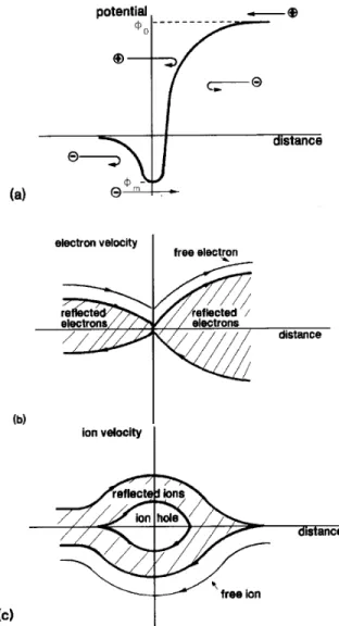
The triplelayer commonly observed in practice is described in this work as the result of ve distinct pop-ulations of charged particles coexisting in equilibrium in some region along the discharge column, viz., an ion beam (free ions) coming from the anode region (the right side of the potential trough), thermal ions which are reected by the potential barrier at the anode re-gion, an electron beam (free electrons) directed from left to right and thermal electrons on the left and on the right of the potential trough (see Fig.1.a). The re-sulting eletrostatic potential prole is determined by the Poisson-Vlasov's system of equations with the free populations assumed to be monoenergetic and the ther-mal ones obeying the Maxwell-Boltzmann distribution. Phase space for both electron populations is illustrated in Fig.1.b. The model presents an ion "hole" in phase space,i.e., there is no thermal ions in the potential trough (see Fig.1.c). The equations are written down in two separate regions along the distance x of the column with the origin (separation plane) at the bottom of the potential trough m, the cathode side on the left with
the eletrostatic potential ! 0 and the anode side on the right with !
0 , the last quantity standing for the at top of the potential barrier; these values are supposed to be known from the experiments. The other relevant quantities in this model are the electron density of the beam directed left to right and near the cathode (at x !,1) ne
0 , the ion density of the beam from right to left and near the anode (at x!+1) ni
0, the electron density and temperature of the thermal elec-trons near the cathode, nec and Tec , and near the
anode, nea and Tea, the ion density and temperature
of the thermal ions ni and Ti , and nally, the electron
and ion beams initial kinetic energies ee0
mev 2
e0=2 and ei0
miv 2
i0=2 , respectively.
Finally, with typical values for temperature and density around 2.eV and 1015m,3, mean free path is about 104cm ,i.e., much larger than the typical layer width observed in the experiments ( cm); also, spe-cial laboratory conditions can provide ionization rate below 1%[8].For these reasons, the layer is assumed to be free of collisions and ionization processes.
Figure 1. (a) A sketch of a triple layer p otential prole withitsvep opulationsindicated bythearrows;(b)phase space fortheelectron p opulation s; (c)phase spaceforthe ionp opulations.
III. The model equations
Having established the basic assumptions,we now write down the various elements leading to Poisson's equation and the Sagdeev potential in analytical forms in two adjacent regions inside the charged region sepa-rately viz., to the left and to the right of the potential minimum.
Firstly, steady-state assumption and continuity equation lead to nebveb = ne0ve0 and nibvib= ni0vi0 for the electron and ion beam respectively and energy conservation applied on each of them leads to
neb= ne0=(1 + 2e=me v 2
e0)
1=2; (1)
and
nib= ni0=[1 + 2e(0
,)=mi v 2
i0]
where the index (0) for the electrons indicates values on the far cathode side (left on the Fig.1a. diagram) and for the ions on the far anode side (right on the same diagram).
According to assumptions, the electron and ion number densities of reected populations are obtained from their velocity distribution functions,
c
fe= ce(me=2 kTe)1=2exp[ ,(mev
2
e=2,e)=kTe]; (3)
fi = ci(mi=2 kTi)1=2exp[ ,(miv
2
i=2 + e)=kTi]; (4)
d where ce and ci are normalization factors to be
de-termined according to the number densities of reected electrons and ions, nec and ni , both dened on the
far cathode side. The distribution function for the elec-trons reected to the right have the same form as in eq.3 but the normalization factor is determined by its number density on the far anode side,nea.
The integrations in velocity space in order to get the number densities are restricted to well dened intervals which depend on the potential prole: for both elec-tron populations ( the one reected to the left and the
other to the right of the potential trough), the limits are (2e=me)
1=2( ,m)
1=2 but for the ion popula-tion, the limits are [2e(
0
,)=mi]
1=2 for > 0 and ,[2e(
0
,)=mi] 1=2 ,
,(,2e=mi)
1=2 together with (,2e=mi)
1=2 , [2e( 0
,)=mi]
1=2 for < 0 , the gap between the two subintervals accounting for the void in phase space of the reected ions (there is no trapped ions in the potential trough). Now, having in mind the even parity of the distribution functions in velocity space and the respective adjustment of the normalization factors, the integrations yields
c
nec() = necexp(e=kTec)erf[e(,m)=kTec]
1=2=erf(
,em=kTec)
1=2; (5)
where m 0 (cathode side, left on Fig.1b diagram), nea() = neaexp[e(,
0)=kTea]erf[e(
,m)=kTea]
1=2=erf[e( 0
,m)=kTea]
1=2; (6)
where m
0 (anode side, right on Fig.1b diagram), Nic() = ni exp(,e=kTi)
erf(e0=kTi) 1=2
ferf[e( 0
,)=kTi] 1=2
,erf(,e=kTi) 1=2
g; (7)
valid for the cathode side (left on Fig.1c diagram) and Nia() = ni exp(,e=kTi)
erf(e0=kTi) 1=2
ferf[e( 0
,)=kTi] 1=2
,H(,)erf(,e=kTi) 1=2
g; (8)
d valid for the anode side (right on the same diagram).In the formulae above,the square roots must be read as applied on the argument of the error function and H
is the usual Heaviside function, used here to describe two distinct expressions for Nia , viz., the one for
is a consequence of the "ion hole" in phase space (see Fig.1c).
Poisson's equation can then be written as (
0 =e)d
2 =dx
2=
neb,nib+nec,Nic (9) and
( 0
=e)d 2
=dx 2=
neb,nib+nea,Nia ; (10) valid forx<0 andx>0 , respectively.
At this point, the following non-dimensional quantities are dened in order to simplify the notation used hereinafter:the normalized potentials
= e=k Tec ,
0 =
e 0
=k Tec and m = em=k Tec , the electron and ion Mach numbers Me = (2ee
0 =k Tec)
1=2 ,
Mi = (2ei 0
=k Tec) 1=2
; the temperature ratiosri=Tec=Ti andra=Tec=Tea , the number density ratios e
0 = ne
0
=nec , i 0 =
ni 0
=nec ,
ea = nea=nec and i = ni=nec and the normalized distance =x=D , where D = (
0
k Tec=nec e 2)1=2 is the Debye lenght and x is the distance measured from the point where = m . Pre-sheat boundary conditions[11] have been circumvented by solving the problem in a Debye's length scale where the innities are located at both ends of the layer.
With notation above[12] , Poisson's equations are integrated from m to making use of the identity
2d 2
=d 2= (
d=d )(d =d)
2 and the boundary condi-tion [d =d] m = 0 . The double integrations implicit in the integration of an error function (erf) are reduced to a single one (another erf) by inversion in the order of integration and the denition of error function (see any recommended textbook of dierential and integral calculus on the topic reduction of multiple integrals). The results for both intervals read,
c d 2 =d 2= e 0
=(1 + 2 =M 2
e)1=2 ,i
0
=[1 + 2( 0
, )=M 2
i]1=2 +e er f( , m)
1=2
=er f(, m) 1=2
,ie ,ri
fer f[ri( 0
, )] 1=2
,er f(,ri ) 1=2
g=er f(ri 0)
1=2
; (11)
(d d
)2= 2 e
0 M
2
e[(1 + 2 =M 2
e)1=2
,(1 + 2 m=M 2
e)1=2] +2i
0 M
2
if[1 + 2( 0
, )=M 2
i]1=2
,[1 + 2( 0
, m)=M 2
i]1=2 g
+ 2
er f(, m) 1=2[
e er f( , m) 1=2
, 2 p
( , m) 1=2
e m]
+ 2i
rier f(ri 0)
1=2 fe
,ri
er f[ri( 0
, )] 1=2
, 2 p
[ri( 0
, )] 1=2
e ,ri
0
,e ,ri m
er f[ri( 0
, m)]
1=2+ 2 p
[ri( 0
, m)] 1=2
e ,ri
0
,e ,ri
er f(,ri )
1=2+ 2 p
(,ri ) 1=2+
e ,ri m
er f(,ri m) 1=2
, 2 p
(,ri m) 1=2
g; (12)
valid for m 0 , 0 and d 2 =d 2= e 0
=(1 + 2 =M 2
e)1=2 ,i
0
=[1 + 2( 0
, )=M 2
i]1=2+ eae
,ra( 0, )
er f[ra( , m)] 1=2
=er f[ra( 0
, m)] 1=2
,ie ,ri
fer f[ri( 0
, )] 1=2
,H(, )er f(,ri ) 1=2
g=er f(ri 0)
1=2
; (13)
(d d
)2= 2 e
0 M
2
e[(1 + 2 =M 2
e)1=2
,(1 + 2 m=M 2
e)1=2] + 2i
0 M
2
if[1 + 2( 0
, )=M 2
i]1=2
,[1 + 2( 0
, m)=M 2
i]1=2 g
+ 2ea
raer f[ra( 0
, m)] 1=2
fe
,ra( 0, )
er f[ra( , m)] 1=2
, 2
p
[ra( , m)] 1=2
e
,ra( 0, m) g+
2i rier f(ri
0) 1=2
fe ,ri
er f[ri( 0
, )] 1=2
2 p
[ri( 0 , )]
1=2e,ri 0
,e
,ri merf[r
i( 0 , m)]
1=2+ 2
p [ri( 0
, m)] 1=2e,ri
0+ H( , )[,e
,ri erf( ,ri )
1=2+ 2 p
(,ri ) 1=2] + e,ri merf(
,ri m) 1=2
, 2 p
(,ri m) 1=2
g: (14)
valid for m 0,
0 .
Now, in order to integrate equations (12) and (14) numerically, boundary conditions (plasma conditions) have to be imposed over the pair of eqns.(11), (12) and (13),(14), viz., d2 =d2= 0 and (d
d)2= 0 , the former pair at (,1) = 0 and the latter at (+1) =
0. The resulting set of equations relating the free parameters reads i= e0
,
i0 (1 + 2 0=M
2
i)1=2 + 1 ; (15)
ea=,
e0 (1 + 2 0=M
2
e)1=2 + i
0; (16)
e0M 2
e[1,(1 + 2 m=M 2
e)1=2] + i0M
2
if(1 + 2 0=M
2
i)1=2
,[1 + 2( 0
, m)=M 2
i]1=2 g+ i
rierf(ri 0) 1=2
ferf(ri 0)
1=2 ,
2 p
(ri 0) 1=2e,ri
0 , e,ri m erf[r
i( 0 , m)]
1=2+ 2 p
[ri( 0 , m)]
1=2e,ri 0+ e,ri merf(
,ri m) 1=2
, 2 p
(,ri m) 1=2
g+ 1, 2 p
(, m) 1=2e m erf(, m)
1=2 = 0 ; (17)
e0M 2
e[(1 + 2 0=M 2
e)1=2
,(1 + 2 m=M 2
e)1=2
] + i0M 2
if1,[1 + 2( 0
, m)=M 2
i]1=2 g+ ea
raerf[ra( 0 , m)]
1=2
ferf[ra( 0
, m)] 1=2
, 2 p
[ra( 0 , m)]
1=2e,ra( 0, m) g+ i
rierf(ri 0) 1=2
f,e
,ri merf[r
i( 0 , m)]
1=2+ 2 p
[ri( 0 , m)]
1=2e,ri 0+ e,ri merf(
,ri m) 1=2
, 2 p
(,ri m) 1=2
g= 0 : (18)
d An additional relation between the electron density of the thermal electrons near the cathode, nec ,and
normalized parameters associated with the beams, can be obtained if the current density J is supposed to be known in the experiment. In this case, we write J=e = ne0ve0+ ni0vi0 , divide by nec (kTec)
1=2 , and make use of the normalized parameters dened before; from the resulting relation one gets
nec= 1:4810 13j=
p tec
e0 Me+ (me=mi) 1=2
i0 Mi
[m,3]; (19) where j and tec are the numerical values of the
(uni-form) current density J in Amps=m2 and the
temper-ature Tec in eV respectively.
be found.
IV.Numerical results and discussion
Now, the boundary conditions together with the additional constraint (19) above, make up ve equations relating the ten free parameters i;e0;i0;ea , Me (or, alternatively, e0 ), Mi (or, alternatively,i0 ), ri (or,alternatively,Ti ), ra;nec and Tec .
Experimental conditions[8] suggest r
i values between
10: and 50: , and the known value of the current den-sity xes the value of nec through relation (19),so that
one ends up with four equations having to be solved for four of these in terms of the other four. We chose e0;i0;ra and Tec as the independent free parameters and ran the computing code, inputing values of the last two for each pair of the rst two. The input values of ra were such as to exclude negative values of densities
in the process of solving the set of boundary conditions. The resulting set of conditions, in its turn, feeds a nu-merical integration scheme for equations (12)and (14) by putting S1=2( ) = d =d and integrating in , i.e.,
=Z
md =S
1=2( ) (20)
where the upper limit in the integration is always kept under 0 for > 0 and under = 0 for < 0 . Invariably in the middle of the numerical process, fur-ther changes on the values of ra were needed so as to
exclude negative values of S.
Fig. 2 illustrates one tipical case, with ; and S standing for the potential, charge density and Sagdeev's potential normalized to kTec , enec and (kTec=D)2 respectively, with the values (see Fig.2) of the input parameters compatible with the experimental condi-tions leading to the formation of charged layers in low pressure mercury-arc discharges(compare with Fig. 4 and 5 in ref.[6]). For all cases run we kept me=mi =
2:71610
,6, J = 1:414 10
4Amps=m2,
0= 24:V olts and m = ,7:5V olts , the rst two used and the last two measured on the axis of the discharge tube[6].
Searching for solution in the parametric space e0 vs:i0 by a double iteration procedure in e0 or i0 and ra and with a xed value of ri (e.g.,ri= 36: ) one nds a region like the one shown in Fig.3 and de-scribed by the curve which limits the minimum values of e0and i0 for solution. The smallest minimum for
e0, the electron beam energy, is limited by the value of ,m (the potential energy barrier for electrons as-sociated with the dip of the potential prole) but the smallest value of i0 depends on the (xed) values of ri and Tec, the last remark also applied to the
asymp-totes to the curve. For relevant values of ri and Tec
other than the one used in the example of Fig.3 how-ever, the new curves constructed on the same basis do not show appreciable departures from it so that one can grossly speaking, take that curve as the representative one which delimits the region in the parametric space e0vs:i0 for solution. Next, for each point (e0;i0) in such a region, the solutions can only be found in its complementary parametric space Tecvs:Tea over a
lim-ited and bounded region (window). The windows were constructed with specic sets of free input parameters borrowed from the ones used in an incomplete model tting the experimental results in ref.[6] so as to allow comparisons. Just two tipical cases are shown in the plots of Fig.4 , viz., window (a) corresponding to the values of (e0;i0) = (30.,16.)eV and window (b) to (31.4,46.)eV. Each of these windows has its boundary represented by two curves having common points at its closure at its lower and upper bound values. Inciden-tally, the inequality i0> Tea=2 is always satised in this model, which is reminiscent of a Bohm's criteria in its inequality form for the onset of a plasma-sheat edge near a negative wall [4] . This imposes an upper limit for Tea which, as a consequence, drives an
up-per bound for Tec . Notice that by xing the value of
ri for each window, one is imposing one further
con-straint on the model. Comparison of windows (a) and (b) of Fig.4 hint at the way the parameters Tec and
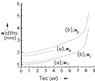
Tea evolve with increasing values of e0and i0, viz., the increase in the range of their values. The widths of the layer for these cases are illustrated in Fig.5, where w1 stands for the length of the region where < 0 and w2 the length joining the two points of maximum , each one averaged over their values in the window for each Tec . Comparison of widths in both windows shows that a signicant increase in widths is obtained the larger the range of denition of Tec, i.e., the larger
the extension of the window along the Tec values. One
can also see that the upper bound for Tec is more
length, representative of the layer, in terms of the rel-evant free parameters, in analitical form. Besides, the entire (graphical) picture would demand a great num-ber of extra computations which might only be appro-priate in a more compreensive version of this work.
Figure 3. A typical solution with initial in-put values i0 = 16:V olts;e0 = 30:V olts;
Tec = 2:eV , iterated ra = :11396 , and calculated
nec= 4:88 10
15m,3;
D=:150mm.
Figure 4. Windows a and b for solutions of the triple layer in the parametric space Tecvs:Tea with
xed values of (e0;i0) = (30.,16.)eV and (31.4,46.)eV
respectively, both with a common value of ri =
36: . Upper bound values for (Tec;Tea) are, for (a),
(4.00,19.19)eV, and for (b), (8.32, 36.18)eV; lower bound values are for (a), (.10, 15.67)eV, and for (b), (.10, 21.76)eV.
Figure 5. Average widths of the triple layer for the windows a and b in Fig.4,w1 standing for the length of the region
where < 0 and w2 the length joining the two points
of maximum , each one averaged over their values in the window for eachTec.
V. Limitation of the model
A close look at the sequence of experimental plots in Fig.10, ref.[7], shows that the potential proles along the direction of the discharge depend strongly on the radial distance from the axis where they were measured. One can see for example that the nearer to the axis the potential were measured the thinner and higher became the prole in the discharge direction. The potential pro-les exhibited show clearly that charge distribution is at least two-dimensional in character and a corresponding 2D model should be more appropriate to describe the layer. Some radial proles would have to be prescribed for the distribution functions of the thermal popula-tions through their parallel and perpendicular temper-atures, along and across the discharge direction as well as for the number densities on the far cathode and an-ode sites. Besides,the maximum and minimum poten-tial should be left to be determined self consistently by the resulting system of equations describing the model. In our 1D model the radial dependency of the charge distribution was circumvented to extend our 1D code to any line parallel to the axis by the prescription of m and
be done at the expense of a reduction on the class of solutions we are looking for, since all the boundary con-ditions on the free parameters have been employed.
A quick comparison of the width of the potential prole exhibitted in Fig.2 (2 mm) with the width of the experimental prole presented at ref.[6] ( 1 cm) might show at a rst sight another limitation of the model. However, the experimental prole has not been presented together with measured parameters associ-ated with all of our free parameters, e.g.,
e0 and
i0; for instance, thicker layer can be found at higher val-ues of
i0 as can be seen from Fig.5. Comparison is made even more dicult for the lack of further exper-imental data and corresponding potential proles. In particular, the ones mentioned in Fig.10, ref.[7], cast some doubts about the precision of the experiments for measurements on the axis (the potential dip in the last plot seems more like a spike). This leaves somewhat undetermined such a comparison and gives no grounds to discard the present model.
As one can infer, the least necessary number of boundary conditions and constraints were used in the present model. Additional boundary condition like
@
@ = 0 at plasma-sheath boundary (
,1;+1 in the present model) [13] or some additional constraint re-stricting the potential proles to some form[6] would reduce the windows regions to lines or even to points, which are done in these works in order to solve their respective model equations in a closed and self consis-tent way. Whatever the physical and mathematicalrea-sons to justify the use of the additional boundary con-dition or constraint (in particular, the mentioned one in ref.[13] does not apply in the present model since the quantity above is singular at those points, unless a non-maxwellian velocity distribution is used), it is not easy to reproduce them in the laboratory, and one might conclude that perhaps windows rather than lines or points would be more like a rule than an exception in practice.
VI. Conclusion
One can say in conclusion that although the results above may seem pertinent to a particular laboratory experiment since most of the input parameters used in the exhibitted graphs in this work have been bor-rowed from the results of an incomplete model whose aim was to try to t them with their experimental re-sults [6] , they are nevertheless representative enough
to validate the model for other aplications. All the ex-hibitted cases will show similar features for any point in the region delimited by the curve shown in Fig.3. By studying the windows boundaries one can draw some conclusions about the relationships of the relevant pa-rameters used in the experiments which would sustain the layer in its steady-state. Even though these rela-tionships are, most of them, of qualitative character, since even the more obvious simplication of the com-plete equations are analitically intractable and there is no Bohm's-like criterion[4] for such a model, the nd-ings in this work may be useful in the sense that they point out the way of establishing the relevant input pa-rameters to be chosen in similar experiments.
Further results and discussion will be published else-where.
Acknowledments
The authors are indebted to Dr.J.E.Allen from the Eng.Dept., Oxford University, UK, for valuable discus-sions.
References
1 I. B. Bernstein, J. M. Greene, M. D. Kruskal, Phys. Rev.108, 546 (1957).
2 W. Schottky, Phys. Zeits.25, 342 (1924).
3 L. Tonks, I. Langmuir, Phys. Rev.34, 876 (1929).
4 D. Bohm D., The characteristics of Electrical Dis-chargesin MagneticFields, ed A. Guthry and R. K.
Wakerling, NY, MacGraw-Hill, 1949.
5 F. W. Crawford, A. B. Canara, J. Appl. Phys.36, 3135
(1965).
6 H. S. Maciel, J. E. Allen, Proc. 2nd Symp. on Plasma Double layers and Related Topics, Insbruck, Austria, pg 218 (1984).
7 H. S. Maciel, J. E. Allen, J. Plasma Physics 42, 321
(1989).
8 H. S. Maciel, PhD thesis, Oxford University, Dept. of engineering Science, Oxford, England, 1985.
9 DeGroot et al., Phys. Rev. Lett.38, 22, 1283 (1977).
10 M. Sanduloviciu, E. Lozneanu, Int. Conf. on Phenom-ena in Ionized Gases, Hoboken, NJ, USA, 1995, ed. Stevens Inst.of Tech., pgs.21-22,172.
11 K-U. Riemann, J. Phys. D: Appl. Phys.24, 493 (1991).
12 H. Yamada, Z. Yoshida, J. Plasma Phys.48, 229 (1992).
13 J. G. Andrews, J. E. Allen, Proc. Roy. Soc. Lond.,A,