Artigos Gerais
On the electrostatic energy of two point charges
(A energia eletrost´atica de duas cargas pontuais)
A.C. Tort
1Instituto de F´ısica, Universidade Federal do Rio de Janeiro, Rio de Janeiro, RJ, Brasil Recebido em 26/11/13; Aceito em 24/2/14; Publicado em 31/7/2014
The electrostatic field energy due to two fixed point-like charges shows some peculiar features concerning the distribution in space of the field energy density of the system. Here we discuss the evaluation of the field energy and the mathematical details that lead to those peculiar and non-intuitive physical features.
Keywords: electrostatic energy, self-energy, classical renormalization.
A energia eletrost´atica de duas cargas puntiformes fixas exibe algumas peculiaridades que dizem respeito `a distribui¸c˜ao da densidade de energia associada ao campo el´etrico total do sistema. Discutimos aqui o c´alculo da energia do ponto de vista do campo e os detalhes que levam a essas caracter´ısticas f´ısicas peculiares e n˜ao intuitivas.
Palavras-chave: eletrost´atica, auto-energia, renormaliza¸c˜ao cl´assica.
1. Introduction
The electrostatic energy of two point charges is given by the simple expression
U12= 1 4πϵ0
q1q2
R , (1)
where R is distance between the charges the values of which are q1 and q2. If the charges have the same al-gebraic sign the electrostatic energy is positive but if the algebraic signs are not equal then the electrostatic energy is negative. Eq. (1) is interpreted as a poten-tial or energy due to the spapoten-tial configuration of the charges. If constraints forces are removed this energy will be transformed into kinetic energy of the charges. On the other hand, from the field point of view the total energy of the system is given by the expression
U = ϵ0 2
∫ ∫ ∫
∥E(P)∥2dV ≥0, (2)
where E(P) is the total field of the system at a point P of the space, that is
E(P) =E1(P) +E2(P). (3) In order to extract the interaction or potential energy of the configuration we must subtract the self-energies of the point charges and next we show how this can be accomplished.
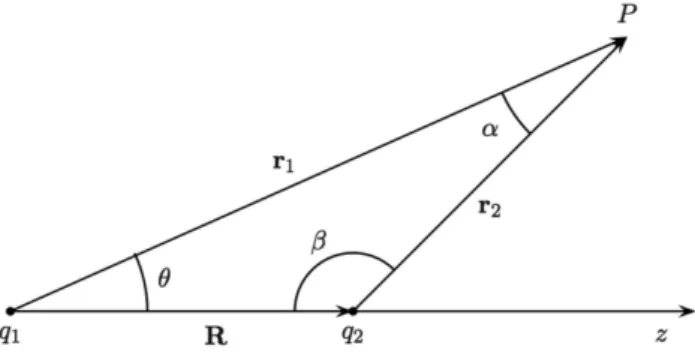
Figure 1 - Geometry for the evaluation of the interaction energy of two point charges.
The field energy can be split into three separate contri-butions
ϵ0 2
∫ ∫ ∫
E2(P)dV =ϵ0 2
∫ ∫ ∫
E21(P)dV + ϵ0
2
∫ ∫ ∫
E22(P)dV +ϵ0
∫ ∫ ∫
E1(P)·E2(P)dV. (4)
The first two terms on RHS of Eq. (4) can be inter-preted as the classical self-energies of the point charges. From a classical point of view both terms lead to diver-gent contributions. To deal with this problem we must introduce a regularization and renormalization scheme. A simple one is to compare two configurations, say the configuration shown in Fig. 1 and the configuration where both point charges are at a different distance, say D, from each other and then subtract one
con-1E-mail: tort@if.ufrj.br.
figuration from the other. This procedure leads to a subtraction of infinities and may cause discomfort even among the not so mathematically-minded. A simple way out of this situation is to replace the point charges by two small identical spherical distributions, for exam-ple, a spherical shell of radiusδuniformly charged with a charge density σ. This is convenient because inside the shells considered one at a time the electric field is zero. This will yield a finite self-energy contribution given by 2×e2/(2·4πϵ
0δ)2. Upon subtraction the self-energy terms will cancel out and we will be left with two crossed terms. Then we let the distance between the two shells in one of the configurations approach in-finity (D→ ∞). This procedure will leave us with one relevant finite crossed term to be calculated. Now we let δ → 0 keeping the charge constant. The surviv-ing crossed term then represents the finite variation of the interaction energy of the two point charges with re-spect to the reference configuration and must reproduce Eq. (1), that is
ϵ0
∫ ∫ ∫
E1(P)·E2(P)dV = 1 4πϵ0
q1q2
R , (5)
but this must be proved by explicit evaluation of integral.
The first time the author heard of this problem was when he was reading the first edition of Ref. [1] where it was proposed as an advanced problem in a special chap-ter at the end of the book. The challenge was to prove that the potential energy point of view and the field energy one were not mutually incompatible by arguing, not necessarily by explicit calculations. Recently, in a paper on the role of field energy in introductory physics courses Hilborn [2] commented on this and some pecu-liar features concerning the distribution in space of the field energy of the system. To appreciate these features consider for simplicity two equal positive charges. Then
1. There is a spherical region centered at one of the charges that does not contribute to the total in-teraction energy.
2. This region can be divided into two subregions that contribute with algebraically opposite ener-gies and the amount of negative energy is very small when compared with the total energy.
3. And, finally, 90% of the field energy lies in a lim-ited part of the space.
Here the present author will try to show to the in-terested reader the details of those peculiar and non-intuitive aspects by performing explicitly the calcula-tions.
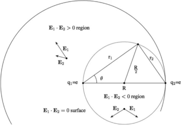
Figure 2 - The distribution of the electrostatic energy density for two similar positive point charges.
2.
Evaluation of the electrostatic
en-ergy
It is convenient to use spherical coordinates with the origin at one of the charges and the polarz-axis along the line that passes through both, see Fig. 1. Let us set q1=q2=e. The crossed term reads
E1·E2= e2 (4πϵ0)2r12r22
er1·er2. (6)
Now we introduce, see Fig. 1
r1=R+r2 (7)
hence
r22=r12+R2−2r1Rcosθ, (8) and, see Fig. 1,
er1·er2 = cosα. (9)
Therefore
E1·E2= e2 (4πϵ0)2
cosα r2
1(r21+R2−2r1Rcosθ)
. (10)
To relateαandθwe apply the sine law to the triangle in Fig. 1
R sinα =
r2
sinθ. (11) Combining this relation with the fundamental trigono-metric identity cos2 α+ sin2 α= 1, we find after some simple manipulations
cosα=
√
1−R
2 r2 2
(1−cos2 θ). (12)
2
Recall that the electrostatic energy associated with a uniformly charged spherical shell whose radius isaand total charge isqis
given by
1 2
q2
Now we take Eq. (8) into the equation above and after some simplifications we get
1−R
2 r2 2
(
1−cos2 θ)
= (r1−Rcosθ) 2 r2
1+R2−2r1R cosθ
. (13)
It follows that
cosα= √ r1−Rcosθ
r2
1+R2−2r1R cosθ
, (14)
and
E1·E2= e2 (4πϵ0)2
r1−Rcosθ r2
1(r21+R2−2r1R cosθ)3/2 . (15)
Therefore we must now compute
U12=ϵ0 × e2 (4πϵ0)2
∫ ∞
0
r21dr1 ×
∫
Ω
r1−Rcosθ r2
1(r21+R2−2r1Rcosθ)
3/2dΩ, (16) where dΩ = sinθ dθ dϕ. The integration over the az-imuthal angle is trivial and yields a factor 2π, and upon introducing the variableξ= cosθ we have
U12= e2 8πϵ0
∫ ∞
0
f(r1)dr1, (17) where we have defined
f(r1) =
∫ +1
−1
r1−R ξ (r2
1+R2−2r1R ξ)3/2
dξ. (18)
This integral can evaluated straightforwardly and be-causeR >0 ,r1>0, we can write the result as
f(r1) = |R−r1|(R+r1)−(R+r1) (R−r1)
|R−r1|(R+r1)r21
. (19)
To proceeed we must consider two cases.
Caser1< R. In this case it is easily seen that
f(r1) = 0. (20) This means that inside of an imaginary sphere of radius equal toR, the interaction energy of the two charges is zero.
Caser1> R. In this case, Eq. (19) yields
f(r1) = 2 r2
1
. (21)
Taking this result into Eq. (17) we obtain the expected result
U12= e 2 4πϵ0
∫ ∞
R
dr1 r2
1 = e
2 4πϵ0R
. (22)
Notice that if we set the upper limit equal to 10R, then a simple calculation shows that
U′
12= e2 4πϵ0
∫ 10R
R
dr1 r2
1 = 9
10 e2 4πϵ0R
, (23)
that is, as stated in Ref. [2], 90% of energy is contained between two spheres, one of radiusRand the other one of radius 10R. If the charges are not identical, all we have to do is replacee2byq
1q2.
3.
The energy density distribution
Though the final result is the one we expected the way it was obtained reveals some details that are some-what surprising, to wit, the part of the field energy that corresponds to the interaction energy of the two point charges comes from the regionr > R. The region r < R makes no contribution at all. This conclusion agrees with Ref. [2]. How can this physically be?
To answer this question we must first realize that the electrostatic interaction energy density of the sys-tem is essentially given by the dot product of the fields. In the case of two positive identical charges it is not difficult to see that the angle between the fields, let us denote it by α as before, is obtuse near the charges and acute far away from them, see Fig. 2. In fact, the negative contributions comes from a spherical region of radius equal toR/2 centered at the midpoint between the two charges, see Fig. 2. The positive contribution comes from the rest. The volume of the spherical re-gion is smaller than the volume of the rest, but the fields are more intense near the charges than far away from them. Therefore, we conclude that in the end there is a cancellation between the corresponding contributions and this is reason why the entire regionr < R makes no contribution at all to the final result. The electro-static field energy of this system comes from the region R < r <∞.
Inside the region r < R there is a surface that separates the negative energy density region from the positve one. On this surface the fields are perpendicu-lar to each other and the energy density is null. This can be seen from Eq. (15). The dot product between the fields is zero if and only if
r1=R cosθ, (24)
spherical surface of radius equal to R/2 the fields are perpendicular to each other and consequently the inter-action energy is zero.
4.
The ratio between negative and
pos-itive energy
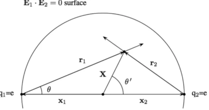
Let us now evaluate the ratio between the negative and the positive field interaction energy. The hard part is the evaluation of the contribution of the negative en-ergy. In order to perform this calculation some geomet-rical transformations will have to be made. Consider Fig. 3. In order to shift the origin of the coordinate system to the midpoint between the charges we intro-duce the position vectors of the charges with respect to the midpoint, x1 and x2, such that x1+x2 = 0 and
∥x1∥ = ∥x2∥ = R/2. We introduce also the position vector X of an arbitrary point P with respect to the midpoint. Notice that the magnitude∥X∥=X of this vector lies in the interval 0≤X≤R/2. The new polar angle isθ′
and the following vector relations are easily seen to hold
Figure 3 - Geometry for the evaluation of the negative energy density contribution.
r1=x2+X; r2=−x2+X. (25) The interaction energy as before depends on the dot product
E1·E2= e2 (4πϵ0)2r21r22
er1·er2 = e 2 (4πϵ0)2r21r22
r1 r1
·r2
r2 .
(26) From the vector relations above it follows that
r21= R2
4 +X
2+RX cosθ′
, (27)
and
r2 2=
R2 4 +X
2−RX cosθ′
. (28)
We also have
r1 r1
·r2
r2 =
X2−R2 4 r1r2
. (29)
Defining the dimensionless variable
u:= X
R, 0≤u≤1, (30)
the field energy content of this regionA12can be writ-ten as
A12=U12
∫ 1/2
0
du u2
(
u2−1
4
)
×
∫ 1
0
dξ
(1
4+u2+u ξ
)3/2(1
4+u2−u ξ
)3/2, (31)
whereξ:= cosθ′
. The integral in ξis
∫ 1
0
dξ
(1
4+u2+u ξ
)3/2 (1
4+u2−u ξ
)3/2 =
64
∥2u−1∥(2u+ 1) (16u4+ 8u2+ 1) , (32) and after performing the integral in uwe obtain
A12=−U12 π−2
4 . (33)
In order to get zero energy inside the spherical region of radiusRcentered at one of the charges we must have an equal amount of a positive contributionB12
B12= +U12 π−2
4 . (34)
Therefore the ratio of the negative energy to the posi-tive energy is
A12 U12+B12
=−
(
π−2 π+ 2
)
≈ −0.2220. (35)
This means that the negative energy content is consid-erable less than the positive energy one.
5.
Final remarks
To conclude let us call the reader’s attention to two points. The first one is that if the point charges have opposite algebraic signs then as before there will still be a sphere centered at one of the charges of radius equal to their separation inside of which the total content of energy is zero, but the energy contained in the smaller sphere of radius R/2 will be positive and the rest of the energy will be negative. This can be easily seen by sketching the dot productE1·E2.
The second one is that all calculations done for the configuration considered here – mutatis muntandis – apply to the corresponding gravitational case. The con-tent of energy stored in the gravitational field is given by
U =− 1
8πG
∫ ∫ ∫
where g(P) is the resultant field at a point P. For a gravitational configuration similar to the electrostatic one considered here g(P) = g1(P) +g2(P), and de-pending on the model we choose for the mass distribu-tion we will not need to deal with infinities due to self-energies.The same can be said about extended charge distributions.
As a final remark, we would like to emphasize that the regularization and renormalization of the divergent self-energy of a point charge is an important problem in classical and quantum electrodynamics, and quan-tum fields in general. For a pedagogical introduction to renormalization in a classical context see Refs. [3, 4]. The reader interested in the quantum aspects of the problem will find plenty of references in the literature. An introduction to its general aspects can be found in Ref. [5]. More technical approaches can be found in Ref. [6]. See also the pioneering work of M. Sch¨onberg in Ref. [7].
Acknowledgments
The author is grateful to the referee and to C. Farina for their helpful comments.
References
[1] E. PurcellElectricity and MagnetismBerkeley Physics Course Vol. 2 1/e See final chapter – Further Problems – Problem 2.30 (McGraw-Hill, New York, 1965).
[2] C.R. Hilborn, ArXiv: 1305.1220.
[3] G. Corb`o, Eur. J. Phys.31, L5-L8 (2010).
[4] A.C. Tort, Eur. J. Phys. 31, L49-L50 (2010).
[5] J.L. Lopes and A. da Silveira, Ciˆencia e Cultura3, 302 (1951)
[6] J.L. Lopes, An. Acad. Bras. Ciˆencias19, 519 (1947).