Exchange Rate Pass-Through in Brazil: Is
There a Relationship?
Reginaldo Pinto Nogueira Junior
∗
Contents: 1. Introduction; 2. A Nonlinear Approach to ERPT; 3. Results; 4. Conclusion.
Keywords: Exchange Rate Pass-Through, Smooth Transition Models.
JEL Code: E31, E52, F41.
Recent studies have suggested that the shift from a high to a low inflation environment induces a decline in the degree of exchange rate pass-through (ERPT) into prices. In this paper we present empirical evi-dence on this matter for Brazil, applying a smooth transition regression model and testing lagged inflation as a potential transition variable. The results presented in this paper go in line with the literature, and suggest that the lower ERPT largely documented for Brazil in recent years may also be a corollary of low and stable inflation.
A literatura recente sugere que a transição de um regime de alta para baixa inflação induz uma redução nopass-throughcambial (ERPT). Neste artigo apresentamos evidência empírica sobre essa questão, utilizando um modelo não-linear comsmooth transition, e testando defasagens da taxa de inflação como variável de transição. Os resultados encontrados corrobo-ram com a literatura sobre o tema, sugerindo que a redução de ERPT ampla-mente documentada para o Brasil em períodos recentes pode ser também uma conseqüência de taxas mais baixas e estáveis de inflação.
1. INTRODUCTION
Several studies have shown that the degree of exchange rate pass-through (ERPT) into prices has declined dramatically in both emerging and developed economies in recent years.1 The most common
explanation for this finding relates it to a lower inflation environment, as proposed by Taylor (2000). He showed that with staggered prices, firms are more likely to pass-through cost changes when inflation is high. In this sense, the degree of ERPT would be endogenous to a country’s inflation performance. Evidence on this relationship was provided by Bailliu and Fujii (2004) and Gagnon and Ihrig (2004)
∗Escola de Governo, Fundação João Pinheiro. Coordenação do Programa de Mestrado da Escola de Governo da Fundação João
markets.
Brazil is an example of country whose ERPT seems to have declined in the past decade (e.g. Nogueira Jr. (2007)). To what extent has a lower inflation environment contributed to this decline is an important question that still needs to be addressed. Hence, the objective of this paper is to present new empirical evidence on ERPT in Brazil, focusing on a possible role for the inflation environment in influencing it. To accomplish this, we take use of a nonlinear smooth transition regression (STR) model and test lagged inflation as a possible transition variable. The STR model allows taking into account that the response of ERPT to changes in inflation may be less than abrupt. In this case, the parameter of the underlying process may evolve continuously, with a smooth transition between the high and low inflation regimes. The results found go in line with the literature, suggesting some degree of influence of the inflation environment on ERPT in Brazil, which we estimate to vary in the long-run from 8% to around 40%, de-pending on the inflation level. Even though this result does not exclude other possible explanations for the decline in ERPT observed in Brazil in the late 1990s, it suggests that the lower inflation environment of the period has had an important role in such decrease, and therefore has been wrongly neglected.2
The remainder of the paper is structured as follows. Section 2 discusses our nonlinear approach to estimating ERPT. Section 3 presents the results. Finally, Section 4 concludes.
2. A NONLINEAR APPROACH TO ERPT
According to Clifton et al. (2001) STR models are a general class of nonlinear time-series models that can account for deterministic changes in parameters over time, combined with regime switching behaviour. The STR model can be roughly described as two weighted average of two linear models, with weights determined by the value of the transition function. The model takes the following general form:
yt=β1xt+β2xtG(st−i,γ,c) +υt (1)
where,st−iis the transition variable,Gis the transition function,γmeasures the speed of transition
from one regime to the other, andcis the threshold for the transition function. The transition function Gis a continuous function bounded between 0 and 1. Asγbecomes larger, the change of the function becomes almost instantaneous.
In this paper we use a particular case of STR models, which is the logistic smooth transition (LSTR). The transition function is given by:
G(st−i,γ,c) =
h
(1 + exp{−γ(St−i−c)})−
1i
(2)
As explained by Christopoulos and León-Ledesma (2007), the LSTR model implies that the nonlinear coefficient takes different values depending on whether the transition variable is below or above the threshold: as(st−c)→ −∞, the coefficient becomesβ1; as(st−c)→+∞the coefficient becomes
β1+β2; and ifst=cit is(β1+β1)/2.
We followed the modelling approach described in van Dijk et al. (2002). First, we tested the null of linearity of a baseline model against smooth transition nonlinearity; if the null was rejected, we estimated the model for which the rejection was the strongest; then, we evaluated the estimated model for general modelling misspecification (including remaining nonlinearity), if the model failed these tests, an extended model was estimated and evaluated.
The estimated model has the following form:
2The most common explanations for the decline in ERPT in Brazil are negative output gaps, greater exchange rate volatility, and
π1 = β0+
n
X
i=1
β1,iπt−i+ n
X
i=0
β2,i∆p∗t−i+ n
X
i=0
β3,iyt−i+ n
X
i=0
β4,i∆et−i+ n
X
i=0
β∗
4,i∆et−i
!
G(st;γ;c) +εt (3)
whereπis the inflation rate,∆p∗is the change in the foreign price of imports,yis the output gap,∆e
is the exchange rate change, andεis an error term. The introduction of foreign import prices follows the previous literature on ERPT. This variable should capture the impact of changes in foreign producer costs on the local currency price of imports.3
Long-run ERPT, or static solution, can be defined as:4
LR=
n
X
i=0
β4,i∆et−i+ n
X
i=0
β∗
4,i∆et−i
!
G(st;γ;c
.
1−
n
X
i=1
β1,iπt−i (4)
Data was obtained from the IMF’s IFS database. We have quarterly data for the period that spans from 1995:01 to 2007:03. All the data is in logs. Exchange rate change data is the change of the national currency per unit of dollar (average of the quarter). A positive variation means depreciation. Import prices are the changes in the series of unit value of imports (in US dollars). Inflation rate is the change of the consumer price index. Finally, output gap is the difference between the seasonally adjusted industrial production index and a trend constructed using the HP Filter. Some ADF unit root tests were applied on these variables, and the results suggest that they can be treated as stationary.
Table 1: ADF unit root tests
Lags t-Statitic p-Value
Exchange rate(∆e) 0 -5,474 0.000
Inflation(π) 1 -4.371 0.001
Output gap(γ) 0 -3.195 0.000
Import prices(∆p∗) 1 -7.440 0.000
Note: Number of lags determined using the Akaike Information Criteria with a maximum of 5 lags.
3. RESULTS
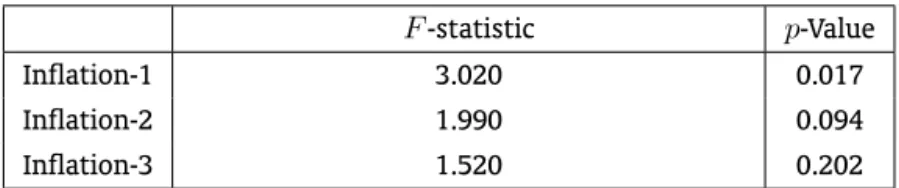
Table 2 provides the results of the linearity tests. Linearity was tested by means of a Lagrange Multiplier (LM) test with the null hypothesis of linearity.5 We tested inflation witht = 1,2,3, as possible transition variable. In Table 2 we present theF-statistics and thep-values of the standard LM test with the different lags for the transition variable.
We then applied the LM test post-estimation, again with the null hypothesis of linearity, in order to test for remaining nonlinearity in the model. The results are in Table 3. Given the combined evidence of Table 2 and Table 3 the chosen transition variable was the one-quarter lagged inflation rate.
3Basically, the price of imports in local currency depends on the price in foreign currency and the exchange rate. Hence,
control-ling for changes in the foreign producer costs allows us to isolate the exchange rate effect. See Campa and Goldberg (2005) for a discussion.
4As long-run ERPT we refer to the cumulative effect of a change in the exchange rate on prices until this effect has died-out.
F-statistic p-Value
Inflation-1 3.020 0.017
Inflation-2 1.990 0.094
Inflation-3 1.520 0.202
Note:F-version of the LM-type linearity test under the null hypothesis of linearity.
Table 3: Remaining nonlinearity tests
F-statistic p-Value
Inflation-1 0.703 0.734
Inflation-2 1.430 0.216
Inflation-3 1.210 0.332
Note:F-version of the LM-type linearity test under the null hypothesis of no remaining nonlinearity.
Table 4 presents the results of the ordinary least squares estimation of the baseline linear model.6
We observe that the linear model passes all the traditional diagnostic tests (including the LM test for autocorrelation,AR); with the exception of theRESETtest for correct functional form. The coefficients have the expected positive sign, and the estimated ERPT is statistically significant. We can think of the coefficients as multipliers: a depreciation of, say, 10% would lead to 0.5% inflation in the following quarter, and to 2.1% inflation over the long-run.
Table 4: Linear ERPT Model
Coefficient Std. error t-statistic
Constant 0.475 0.239 1.990
Inflation-1 0.534 0.154 3.470
Inflation-2 0.074 0.140 0.530
Exchange rate 0.031 0.016 1.980
Exchange rate-1 0.050 0.018 2.860
Import prices-1 0.003 0.006 0.473
Output-1 0.013 0.055 0.237
Linear Long-run ERPT 0.208
R-squared 0.573 Normality test 2.775
AR 1-4 test 2.054 RESET test 4.302
ARCH 1-4 test 1.013 Hetero test 1.365
Table 5 shows the results of the nonlinear least squares estimation of the LSTR model. The com-parison of the results of the linear and the nonlinear models shows that the latter provides a better fit to the data. TheR-squared obtained from the LSTR model is 0.71, whereas the one obtained from the linear model is just 0.57. The nonlinear model passes the diagnostic tests applied, this time including
Table 5: Nonlinear ERPT Model
Coefficient Std. error t-statistic
Gamma 3.892 3.163 1.230
Threshold 2.556 0.320 8.001
Constant 0.625 0.220 2.841
Inflation-1 0.239 0.169 1.501
Inflation-2 0.228 0.136 1 .677
Exchange rate 0.034 0.016 2.165
Exchange rate-1 0.010 0.041 0.239
Import prices-1 0.007 0.006 1.199
Output-1 -0.038 0.052 -0.721
Nonlinear Parameters
Exchange rate -0.057 0.050 -1.151
Exchange rate-1 0.220 0.063 3.503
Nonlinear Long-run ERPT
G(transition function) = 1 0.388 G(transition function) = 0 0.083
R-squared 0.714 AR 1-4 test 1.660
RESETtest 0.641 Akaike Info Criteria -0.511
the RESET test for correct functional form. These results reinforce the argument that ERPT should be modelled nonlinearly and that inflation is a viable transition variable.
As argued before we expect that ERPT will be lower under a better inflation environment, i.e. lower lagged inflation. Looking at the nonlinear parameters of the LSTR model we observe that this is the case for Brazil. The sum of the nonlinear coefficients is highly positive, although the coefficient of the contemporaneous effect is negative. This high value of the sum of the nonlinear coefficients (0.163) indicates a strong influence of inflation on ERPT in Brazil.
Let’s now turn our attention to the threshold. It shows that ERPT will enter the high inflation regime when the quarterly inflation rate is around 2.56%, or approximately 10.6% at an annualized rate. When inflation is above the threshold and the transition function (G) is equal to 1, the one-period lagged ERPT is 0.27, whereas the long-run effect is about 0.39. It means that, under those circumstances, a depreciation of, say, 10% would lead to 2.7% inflation in the next quarter, and almost 4% in the long-run. On the other hand when inflation is well below the threshold, and the transition function is equal to 0, long-run ERPT will be as low as 0.08, so a depreciation of 10% would lead to just 0.8% inflation in the long-run.
to 0, and therefore the lower ERPT is.
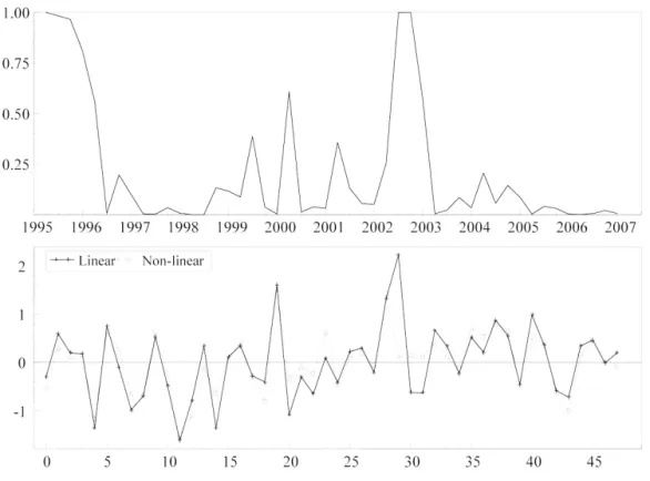
Figure 1: Transition function, and error terms
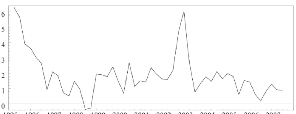
Figure 2 shows the evolution of the transition variable (inflation) over time. Comparing the figures of the transition function and the transition variable allows observing the evolution of ERPT through time, as well as the corresponding change in inflation. ERPT reached its maximum level during the first years of the sample, which correspond to the quarters immediately after the inflation stabilization brought about by the Real Plan. After that, both ERPT and inflation fluctuated considerably, but always at lower level than before. It is important to bear in mind that the Inflation Targeting framework was adopted in Brazil in mid-1999, but inflation has exceeded the target in several quarters. In the final quarters of 2002 ERPT reached its maximum level once again, when a huge confidence crisis stormed the country. After 2003 inflation was once again stabilized, and therefore the observed ERPT is very low, particularly in the last two years of the sample when inflation seems to have been tamed by the Central Bank.
Summing up, the results presented here support empirically the view of the recent literature, as we have found that a lower inflation environment is an important determinant of ERPT in Brazil.
4. CONCLUSION
Figure 2: Transition variable
by a successful monetary policy. This is a strong argument in favour of pursuing low and stable rates of inflation, as it demonstrates that once inflation is stabilized at low levels the inflationary impacts of depreciations will also be lower, making it easier and less costly to maintain the inflation stability. Although we do not discard other determinants of ERPT, such as measures of economic activity and exchange rate volatility, we believe that the role of low inflation has been mistakenly neglected.
BIBLIOGRAPHY
Bailliu, J. & Fujii, E. (2004). Exchange rate pass-through and the inflation environment in industrialized countries: An empirical investigation. Bank of Canada Working Paper 21.
Campa, J. & Goldberg, L. (2005). Exchange rate pass-through into imports prices. Review of Economics and Statistics, 87:679–690.
Ca’Zorzi, M., Hahn, E., & Sánchez, M. (2007). Exchange rate pass-through in emerging markets. Euro-pean Central Bank Working Paper 739.
Choudhri, E. & Hakura, D. (2006). Exchange rate pass-through to domestic prices: Does the inflationary environment matter? Journal of International Money and Finance, 25:614–639.
Christopoulos, D. & León-Ledesma, M. (2007). A long-run nonlinear approach to the Fischer effect.
Journal of Money, Credit and Banking, 39:543–559.
Clifton, E., Leon, H., & Wong, C. (2001). Inflation targeting and the unymployment-inflation trade-off. International Monetary Fund Working Paper 166.
Gagnon, J. & Ihrig, J. (2004). Monetary policy and exchange rate pass-through. International Journal of Finance and Economics, 9:315–338.
Nogueira Jr., R. (2007). Inflation targeting and exchange rate pass-through. Economia Aplicada, 11:189– 208.