Quantifying the sub-grid variability of trace gases and aerosols based on WRF-Chem simulations

(1)

ACPD

10, 10777–10837, 2010

Quantifying sub-grid variability of trace gases and aerosols

Y. Qian et al.

Title Page

Abstract Introduction

Conclusions References

Tables Figures

◭ ◮

Back Close

Full Screen / Esc

Printer-friendly Version

Interactive Discussion

Atmos. Chem. Phys. Discuss., 10, 10777–10837, 2010 www.atmos-chem-phys-discuss.net/10/10777/2010/ © Author(s) 2010. This work is distributed under the Creative Commons Attribution 3.0 License.

Atmospheric Chemistry and Physics Discussions

This discussion paper is/has been under review for the journal Atmospheric Chemistry and Physics (ACP). Please refer to the corresponding final paper in ACP if available.

Quantifying the sub-grid variability of

trace gases and aerosols based on

WRF-Chem simulations

Y. Qian, W. I. Gustafson Jr., and J. D. Fast

Atmospheric Sciences and Global Change Division, Pacific Northwest National Laboratory, Washington, USA

Received: 30 March 2010 – Accepted: 13 April 2010 – Published: 23 April 2010 Correspondence to: Y. Qian ([email protected])

(2)

ACPD

10, 10777–10837, 2010

Y. Qian et al.

Title Page

Tables Figures

◭ ◮

Back Close

Full Screen / Esc

Abstract

One fundamental property and limitation of grid based models is their inability to identify spatial details smaller than the grid cell size. While decades of work have gone into de-veloping sub-grid treatments for clouds and land surface processes in climate models, the quantitative understanding of sub-grid processes and variability for aerosols and

5

their precursors is much poorer. In this study, WRF-Chem is used to simulate the trace gases and aerosols over central Mexico during the 2006 MILAGRO field campaign, with multiple spatial resolutions and emission/terrain scenarios. Our analysis focuses on quantifying the sub-grid variability (SGV) of trace gases and aerosols within a typical global climate model grid cell, i.e. 75×75 km2.

10

Our results suggest that a simulation with 3-km horizontal grid spacing adequately reproduces the overall transport and mixing of trace gases and aerosols downwind of Mexico City, while 75-km horizontal grid spacing is insufficient to represent local emis-sion and terrain-induced flows along the mountain ridge, subsequently a_ffecting the transport and mixing of plumes from nearby sources. Therefore, the coarse model grid

15

cell average may not correctly represent aerosol properties measured over polluted areas. Probability density functions (PDFs) for trace gases and aerosols show that secondary trace gases and aerosols, such as O3, sulfate, ammonium, and nitrate, are

more likely to have a relatively uniform probability distribution (i.e. smaller SGV) over a narrow range of concentration values. Mostly inert and long-lived trace gases and

20

aerosols, such as CO and BC, are more likely to have broad and skewed distributions (i.e. larger SGV) over polluted regions. Over remote areas, all trace gases and aerosols are more uniformly distributed compared to polluted areas. Both CO and O₃SGV ver-tical profiles are nearly constant within the PBL during daytime, indicating that trace gases are very efficiently transported and mixed vertically by turbulence. But,

simu-25

(3)

ACPD

10, 10777–10837, 2010

Y. Qian et al.

Title Page

Tables Figures

◭ ◮

Back Close

Full Screen / Esc

and secondary aerosols reaches a maximum at the PBL top during the day. The SGV decreases with distance away from the polluted urban area, has a more rapid decrease for long-lived trace gases and aerosols than for secondary ones, and is greater during daytime than nighttime.

The SGV of trace gases and aerosols is generally larger than for meteorological

5

quantities. Emissions can account for up to 50% of the SGV over urban areas such as Mexico City during daytime for less-reactive trace gases and aerosols, such as CO and BC. The impact of emission spatial variability on SGV decays with altitude in the PBL and is insignificant in the free troposphere. The emission variability affects SGV more significantly during daytime (rather than nighttime) and over urban (rather than rural or

10

remote) areas. The terrain, through its impact on meteorological fields such as wind and the PBL structure, affects dispersion and transport of trace gases and aerosols and their SGV.

1 Introduction

One fundamental property and limitation of all Eulerian models is their inability to

iden-15

tify spatial details smaller than the grid cell size, known as sub-grid variability (SGV). SGV is present for meteorological variables as well as trace gases and aerosols, even when very small grid spacings are employed (Haywood et al., 1997; Karamchandani, et al., 2002; Ching et al., 2006). For weather and climate models, with grid spacing rang-ing from a few to hundreds of kilometers, the SGV of meteorological variables arises

20

from within-grid variability of terrain, land surface type and properties, and clouds. For example, Leung and Qian (2003) found that spatial resolution has a significant impact on simulation results over mountainous areas in the western US Higher spatial resolu-tion improves the simularesolu-tion, especially for orographic precipitaresolu-tion and snowpack, due to better reproduction of the temperature gradient by resolving the complex terrain and

25

(4)

ACPD

10, 10777–10837, 2010

Y. Qian et al.

Title Page

Tables Figures

◭ ◮

Back Close

Full Screen / Esc

effects of the sub-grid terrain variability itself.

For chemistry models, the SGV of trace gases and aerosols results from both the traditional sub-grid processes affecting meteorology and specific chemistry processes, such as emissions, chemical transformation, and removal. In most chemistry models, primary emissions are usually instantaneously and uniformly diluted over an entire grid

5

cell volume. In the real world, the spatial distribution of anthropogenic emissions (e.g. SO2, NOx, CO, black carbon, organic matter) from point, area, and mobile sources

are quite inhomogeneous and dissimilar within a model grid cell. Models that currently employ grid spacings of 1 to 100 km cannot resolve all the small-scale variations in anthropogenic, biomass burning, and biogenic emissions. In addition, the subsequent

10

dispersion and mixing of trace gas and aerosol plumes in the horizontal and vertical dimensions occurs at highly variable rates. Different spatial resolutions may result in different predictions of secondary products such as ozone and sulfates, since many atmospheric chemistry processes are nonlinear and frequently di_ffusion-limited.

Climate models in the Intergovernmental Panel on Climate Change Fourth

Assess-15

ment Report typically employ a horizontal grid spacing on the order of 100 km. This is much larger than the width of pollution plumes near source regions, such as power plant stacks (e.g. Chapman, et al., 2009), and also larger than the spatial scales of many of the other processes causing aerosol spatial variability, such as aqueous gener-ation and scavenging of aerosol induced by cloud, and transport and mixing influenced

20

by terrain features. While the reduction of grid spacing is foreseen in future model-ing activities, the question of how much resolution is needed to accurately reproduce aerosol impacts on climate is not known.

Another confounding factor when evaluating climate or chemistry models is the com-parison of point measurements with model grid cell averages. This is considered a

25

(5)

ACPD

10, 10777–10837, 2010

Y. Qian et al.

Title Page

Tables Figures

◭ ◮

Back Close

Full Screen / Esc

different choice in the size of the grid cell chosen for the simulation. Moreover, any ob-servation reflects an instantaneous event out of a population, while model predictions represent an average of the population during a time step. When SGV is significant, the comparison of grid model outputs against one or more point measurements can result in comparisons seeming worse than they really are (Ching et al., 2006; Touma

5

et al., 2006).

Decades of work have gone into developing sub-grid treatments for clouds or land surface process in climate models (Slingo, 1980; Randall et al., 2003; Avissar and Pielke, 1989; Seth et al., 1994). It has come to be accepted that high resolution is needed to improve the handling of clouds in climate models (e.g. Shukla, et al., 2009).

10

The quantitative understanding for sub-grid processes and variability of aerosols and their precursors are much poorer. For example, is the same resolution needed for aerosols as for clouds to resolve the SGV? If aerosols could be modeled at a coarser resolution than the clouds, a significant savings could be had since many more vari-ables must be stored and advected for the aerosols and the associated trace gas

chem-15

istry than are needed for the traditional meteorological fields. Quantification of sub-grid variability of aerosols and better understanding of the extent to which different sub-grid-scale processes contribute to uncertainty in aerosols and their radiative forcing within climate models are needed to assist in developing parameterization schemes that could account for at least a portion of the neglected sub-grid aerosol processes in

20

these models.

While a systematic approach has not yet been employed to document the impact of neglected subgrid aerosol variability, some work has been done to parameterize it. The most prominent of these attempts is the plume-in-grid concept, which was ini-tially developed for the handling of ozone plumes within a grid cell (Karamchandani,

25

(6)

ACPD

10, 10777–10837, 2010

Y. Qian et al.

Title Page

Tables Figures

◭ ◮

Back Close

Full Screen / Esc

models (Gustafson et al., 2008). This latter technique uses statistics from high resolu-tion cloud models embedded within each coarse GCM column to improve the treatment of vertical mixing and cloud processing of aerosols.

In this study, the chemistry version of the Weather Research and Forecasting model (WRF-Chem) is applied to simulate the aerosols and other trace gases over the vicinity

5

of Mexico City during the 2006 Megacity Initiative: Local and Global Research Obser-vations (MILAGRO) using multiple spatial resolutions and scenarios that examine the effect of SGV of emissions and terrain. Our analysis in this study focuses on quanti-fying the sub-grid variability of trace gases and aerosols within a typical global climate model (GCM) grid cell, i.e. 75×75 km. Nested domains with grid spacing representative 10

of mesoscale models (i.e. 15 km), and cloud-system resolving models (i.e. 3 km) are used to identify how the simulated aerosol characteristics change with spatial scale. The paper is organized as follows: in Section 2 we briefly introduce the WRF-Chem model configuration, experiment design, and observational data. In Section 3 we eval-uate WRF-Chem simulations at various spatial resolutions against observations, with

15

the objective of quantifying the uncertainty caused by spatial variability for trace gases and aerosols when comparing point measurements to grid cell volumes at di_fferent spatial resolutions. In Section 4 we present the basic characteristics of the SGV of trace gases and aerosols, including their spatial pattern, diurnal and vertical variation, and dependences on the distance to emission sources and on the spatial resolution. In

20

Section 5, based on a series of sensitivity experiments, we analyze the factors aff ect-ing sub-grid scale processes, includect-ing local forcect-ings such as topography and emission variability. Conclusions and discussions are presented in Section 6. The results of this study improve our understanding of sub-grid process of trace gases and aerosols and provide useful information guiding parameterization development designed to reduce

25

(7)

ACPD

10, 10777–10837, 2010

Y. Qian et al.

Title Page

Tables Figures

◭ ◮

Back Close

Full Screen / Esc

2 WRF-Chem and experiment design

2.1 Model description

The non-hydrostatic Weather Research and Forecasting (WRF) community model in-cludes various options for dynamic cores and physical parameterizations so that it can be used to simulate atmospheric processes over a wide range of spatial and

tempo-5

ral scales (Skamarock et al., 2008). WRF-Chem, the chemistry version of the WRF model (Grell et al., 2005), simulates trace gases and particulates interactively with the meteorological fields. WRF-Chem contains several treatments for photochemistry and aerosols developed by the user community.

The modules in WRF-Chem version 3 used in this study are: the CBM-Z gas-phase

10

chemistry mechanism (Zaveri and Peters, 1999), the MOSAIC aerosol model that em-ploys a sectional approach for the aerosol size distribution (Zaveri et al., 2008), and the Fast-J photolysis scheme (Wild et al., 2000). The aerosol direct effect is coupled to the Goddard shortwave scheme (Fast et al., 2006). The interactions between aerosols and clouds, such as the first and second indirect e_ffects, activation/resuspension, wet

15

scavenging, and aqueous chemistry (Gustafson et al., 2007; Chapman et al., 2009), are not turned on. Aerosol-cloud interactions were probably negligible prior to the cold surge on 23 March when mostly sunny conditions were observed over the central Mexican plateau (Fast et al., 2007). Prognostic species in MOSAIC include sulfate, nitrate, ammonium, chloride, sodium, other (unspecified) inorganics, organic matter

20

(OM), black carbon (BC), aerosol water, and aerosol number. Eight size bins are used for each aerosol specie. Aerosols are assumed to be internally mixed and volume-averaging is used to compute optical properties that influence radiation. It should be noted that no secondary organic aerosol (SOA) treatment is included in the version of MOSAIC used for this paper. The configuration of WRF-Chem is similar to Fast et al.

25

(8)

ACPD

10, 10777–10837, 2010

Y. Qian et al.

Title Page

Tables Figures

◭ ◮

Back Close

Full Screen / Esc

among domains with different resolutions so that the results would not be directly com-parable. We therefore chose to neglect data assimilation because it would confound the interpretation of SGV of trace gases and aerosols.

The following meteorological physics options were employed: the Rapid Radiative Transfer Model (RRTM) for longwave (Mlawer et al., 1997), the Goddard shortwave

5

scheme (Chou and Suarez, 1994), the Noah land surface model (Chen and Dudhia, 2001) for land surface processes, the Kain-Fritsch cumulus and shallow convection scheme (Kain, 2004) (for domains with grid spacing greater than 10 km), the Yonsei University nonlocal boundary layer turbulence transfer scheme (Hong et al., 2006), and the Lin mixed phase cloud microphysics scheme. Advection included the positive

10

definite limiter (Skamarock, 2006) for both the water and chemistry species as was found necessary by Chapman et al. (2009) to prevent spurious mass production.

2.2 Experiment design

The period of the simulations, from 06:00 UTC (00:00 LT, Local Time) 1 March to 06:00 UTC 30 March, coincides with most of the airborne and surface measurements

15

during MILAGRO. Only the results from 00:00 UTC 5 March to 00:00 UTC 30 March are averaged and used in the analysis shown later in this paper. Two computational domains are employed. The larger domain, which encompasses Mexico, Southern Texas, and a portion of Central America, has 75-km grid spacing. A smaller domain, encompassing central Mexico, a portion of the Gulf of Mexico and includes a large

frac-20

tion of the aircraft flight paths is used with smaller grid spacings. Simulations for the smaller domain use either 3-km or 15-km grid spacing. The analysis is conducted for a series of four locations that lie along the dominant synoptic flow pattern from Mexico City towards the Gulf of Mexico, with each station farther from the large source of emis-sions over Mexico City. The sites are referred to as T1, representing an area of large

25

(9)

ACPD

10, 10777–10837, 2010

Y. Qian et al.

Title Page

Tables Figures

◭ ◮

Back Close

Full Screen / Esc

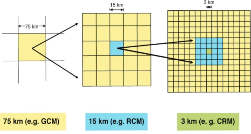
The 3-km and 15-km domains are setup with identical corner locations that coincide with the corners of cells on the 75-km grid. Each grid cell in the 75-km simulation consists of a 5×5 set of cells in the 15-km grid, and each grid cell in 15-km simulation

consists of a 5×5 set of cells in 3-km simulation (see Fig. 1). This allows us to easily

compare values over equivalent regions between grids. The statistics comparing the

5

high- and low-resolution grids are all for a 75 km by 75 km square equivalent to the grid cell from the 75-km grid cell containing the site. We define this area as GC75. For the 75-, 15-, and 3-km grids, the resulting area contains 1, 25, and 625 cells, respectively, that can contribute to variability within the region.

To ensure identical boundary forcings to the central region of the 75-km grid where

10

all three grids cover identical areas, the initial and boundary conditions are handled differently between the 75-km and the other two grids. For the 75-km grid, initial and boundary conditions are provided at 6 h intervals for the meteorological variables from the National Center for Environmental Prediction’s Global Forecast System (GFS) model on a 1 by 1-degree grid; the initial and boundary conditions for the trace gas

15

and aerosol species are provided every 6 h by the MOZART-4 global chemistry model (Pfister et al., 2008) as in Fast et al. (2009). Initial and boundary conditions for mete-orological, trace gas, and aerosol variables for the 15-km and 3-km grids are derived once per hour from the 75-km grid using one-way nesting. This procedure ensures that the large-scale forcing for the region of comparison is identical, allowing us to attribute

20

di_fferences between the simulations to local impacts and SGV derived from di_fferences between the grid resolutions.

Emissions for this study are identical to those used by Fast et al. (2009) with the exception that they have been regridded to the domains used in this study. Emissions of anthropogenic trace gases and particulates were obtained from two inventories: the

25

(10)

ACPD

10, 10777–10837, 2010

Y. Qian et al.

Title Page

Tables Figures

◭ ◮

Back Close

Full Screen / Esc

(http://www.epa.gov/5ttn/chief/net/mexico.html). Emissions of CO, NO_x, SO₂, VOC, NH3, PM2.5, and PM10are available for point, area, and mobile sources. The right

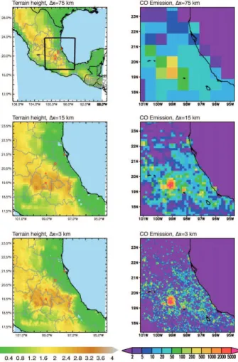
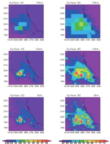
col-umn of Fig. 2 illustrates the area emission of CO for the three grid spacings. Biomass burning emissions are included and are based on the MODIS thermal anomalies prod-uct (Wiedinmyer et al, 2006). Biogenic emissions were calculated using the MEGAN

5

v2.04 model. Dust emissions were calculated interactively during the model simulation based on grid cell wind speed, moisture, and other relevant conditions using the dust module in WRF-Chem based on Shaw et al. (2008) (Zhao et al., 2010). Note that be-cause the dust and biogenic emissions are determined interactively during the model simulation, the total mass of emitted dust differs between domains, whereas the mass

10

of other emissions is consistent between the three grids for equivalent areas.

Table 1 summarizes the experiments done in this study. C75, C15, and C3 are control simulations, in which the model configuration is identical except for the grid spacings of 75 km, 15 km, and 3 km, respectively. E15 is the same as C15 except that the anthropogenic and biomass burning emissions are on the 75-km grid instead

15

of the 15-km grid, i.e. with a uniform emission over each GC75. E15 is a sensitivity experiment to test the e_ffect of emissions on SGV of trace gases and aerosols. T15 has everything the same as C15 except that the 15-km terrain is replaced with the 75-km terrain. This results in a flat terrain over each GC75, and serves as a sensitivity experiment to test the e_ffect of terrain on SGV of trace gases and aerosols.

20

2.3 Observational data

The Mexico City metropolitan area (MCMA), with a population of ∼20 million, is the

largest metropolitan area in North America and is located within a basin on the central Mexican plateau at an elevation of 2200 m above sea level. Mountain ranges that are

∼1000 m higher than the basin floor border the west, south, and east sides of the city, 25

(11)

ACPD

10, 10777–10837, 2010

Y. Qian et al.

Title Page

Tables Figures

◭ ◮

Back Close

Full Screen / Esc

Air pollution in MCMA has been studied for many years (Raga et al., 2001; Salcedo, 2006; Molina et al., 2007). MILAGRO, composed of several collaborative field exper-iments supported by various Mexican institutions and the US National Science Foun-dation (NSF) and Department of Energy (DOE), is the largest of a series of campaigns in and around the MCMA (Molina et al., 2008). The month of March was selected for

5

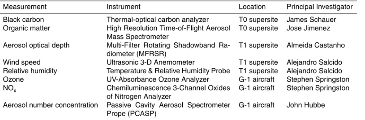
the field campaign period because of the dry, mostly sunny conditions observed over Mexico at this time of the year. A comprehensive set of meteorological, trace gas, and aerosol measurements were obtained at the surface and aloft over a wide range of spatial scales. Extensive surface chemistry and meteorological profiling measure-ments were made at three “supersites” denoted by T0, T1, and T2, of which the latter

10

2 are shown in Fig. 2 (e.g. Doran et al., 2007; Shaw et al., 2007). A detailed list of instruments and instrument platforms is given in Molina et al. (2010) and research find-ings derived from the measurements have been in a special section ofAtmospheric

Chemistry and Physicsat http://www.atmos-chem-phys.org/special issue83.html.

The observations used in this study were collected by the many scientists who

par-15

ticipated in MILAGRO, and were ported into the Aerosol Modeling Testbed (AMT) de-veloped at the Pacific Northwest National Laboratory (http://www.pnl.gov/atmospheric/ research/aci/amt/). The AMT (Fast et al., 2010) collects all the MILAGRO measure-ments into a central location and reformats the data into a single format, significantly reducing the time needed for analysis and graphing (Rishel et al., 2009). Table 2

high-20

lights the primary data used in this study, which consists of surface observations at the T0 and T1 MILAGRO supersites and measurements from the DOE G-1 aircraft.

3 Evaluation of WRF-Chem simulations at various spatial resolutions against observations

We first compare the performance of the model at various spatial resolutions. Fast

25

(12)

ACPD

10, 10777–10837, 2010

Y. Qian et al.

Title Page

Tables Figures

◭ ◮

Back Close

Full Screen / Esc

meteorology, trace gases, and aerosols during MILAGRO, with the simulations by Fast most closely resembling those in this study. Here we focus on comparing the present simulations against observations, with the objective of investigating uncertainty that arises from comparing point measurements to model grid cell estimates at different grid spacing.

5

3.1 Meteorological fields

High-pressure systems, weak synoptic forcing in the sub-tropics and horizontal temper-ature gradients over the central Mexican plateau are favorable for the development of local and regional thermally-driven flows (Fast et al., 2007). Several studies have eval-uated simulations of near-surface winds and PBL structure over the MCMA (e.g. Fast

10

and Zhong, 1998; de Foy et al., 2006). It remains a challenging task to simulate the details of near-surface winds at specific locations and times over areas with complex terrain, whereas most mesoscale models can capture the primary thermally-driven cir-culations and their interaction (Zhang et al., 2009). As summarized in Fast et al. (2007) and de Foy et al. (2008), clear skies, low humidity, and weak winds aloft associated

15

with high-pressure systems are usually observed over Mexico during March. The near surface winds over the central Mexican plateau are influenced by the thermally-driven circulation associated with terrain and large-scale synoptic flow. The thermal and dy-namic effects of urbanization and aerosols also modify boundary layer properties (Jau-regui, 1997) and subsequently near-surface transport and mixing of pollutants.

20

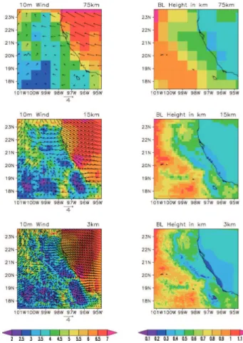
Wind Speed – The left column of Fig. 3 shows the near-surface wind fields (10-m

height) in C75, C15, and C3, averaged from 5 to 30 March. Generally, the wind speed is less than 4 m s−1 _{over land. The di}

fferences for wind speed and direction among the three simulations are smaller over the ocean and coastal plains where the surface is flat. In contrast, C75 is incapable of capturing many local wind features associated

25

(13)

ACPD

10, 10777–10837, 2010

Y. Qian et al.

Title Page

Tables Figures

◭ ◮

Back Close

Full Screen / Esc

central and southern Mexico since it better captures the local thermally-driven down-slope and up-down-slope flows due its higher spatial resolution. Small-scale heating and terrain geometry associated with the mountain ranges leads to local-scale circulations. While different wind patterns associated with various synoptic conditions (e.g. cold surge events) occurred during March (Fast et al., 2007), southerly winds can be found

5

in the vicinity of Mexico City when averaged from 5 to 29 March. Indeed, Fast et al. (2007) suggested that the Mexico City pollutant plume is transported northeastward 20–30% of the time during March.

The left column of Fig. 4 compares the observed and simulated wind speed at T1. Associated with the change of PBL structure, the near-surface wind speed over Mexico

10

City exhibits a strong diurnal cycle, with minimum wind speed during early morning and a maximum during late afternoon. The observed wind is between 1-5 m s−1 _{most of}

time and the maximum wind speed is less than 10 m s−1_{. The magnitude and variability}

of wind speed at T2 is similar to T1. While all three simulations capture the diurnal cycle of wind speed, C75 significantly underestimates the variability and diurnal range

15

of wind speed. C75 underpredicts the maximum wind speed by 40-50% during late afternoon and overpredicts the minimum wind speed during morning. As shown in Fig. 4, C3 and C15 capture the peak wind speed most days. It should be noted that it remains a difficult task to quantitatively compare the simulated wind speed at a specific location and time with the observation, especially when wind speed is low (Zhang et

20

al., 2009). Surface wind measurements in an area with a complex underlying surface are not likely to be representative of a larger area.

PBL Height– The PBL height (PBLH) is often used to describe the depth of the

ver-tical mixing that a_ffects the dispersion of pollutants. Mixing heights during the MCMA-2003 campaign reached around 3000 m and vigorous vertical mixing implied pollutants

25

(14)

ACPD

10, 10777–10837, 2010

Y. Qian et al.

Title Page

Tables Figures

◭ ◮

Back Close

Full Screen / Esc

simulated variation and magnitude of PBLH are very similar over T1 and T2, which is consistent with the measurements of Doran et al. (2007). It has been noted that the YSU PBL scheme used in WRF has a tendency to collapse the afternoon PBL too quickly (Fast et al., 2009).

The right column of Fig. 3 compares the simulated PBLH for the three spatial

reso-5

lutions. Since PBLH is strongly influenced by the terrain, the detailed features of PBLH over mountainous areas are not captured in C75. Generally, PBLH is higher over the southwestern portion of the grids and gradually decreases to the northeastward as shown in all three simulations, with the lowest values over the Gulf of Mexico. C75 overpredicts the PBLH over the eastern coastal plains and fails to capture the minimum

10

PBLH along 19◦_{N near MC.}

Relative Humidity – Relative humidity (RH) is an important meteorological variable

because it directly affects uptake and evaporation of aerosol water, thus significantly a_ffecting the optical properties of aerosols. The right column of Fig. 4 compares the observed and simulated RH at T1. A significant diurnal cycle for RH is found in both

15

the observations and simulations. The RH is usually lower than 60% before 15 March, and afternoon minimum RH often drops to below 10%. The daily maximum RH rises to above 80% around 15 March because of an El Norte event, which transports moisture to the plateau from the Gulf of Mexico. The averaged RH, especially maximum RH during later nighttime, is higher during the second half of the month than during the

20

first half of month.

All three simulations reproduce the diurnal cycle of RH, with the maximum value associated with a lower temperature and a shallower PBL around sunrise and the min-imum value associated with a higher temperature and a deeper PBL during afternoon. However, C75 overpredicts maximum RH by 20–30% and minimum RH by 5–15%,

re-25

(15)

ACPD

10, 10777–10837, 2010

Y. Qian et al.

Title Page

Tables Figures

◭ ◮

Back Close

Full Screen / Esc

decreases to southwestward as shown in all three simulations, with lowest RH over the central Mexican plateau.

3.2 Trace gases

CO– The chemical lifetime of carbon monoxide (CO) is about 2 months, thus over the few days relevant here it can be considered as a passive tracer that is emitted from the

5

surface, mixed in the PBL, and transported by the prevailing winds (Tie et al., 2009). We first examine the predictions of CO to evaluate the impact of transport on the SGV of trace gases. Fast et al. (2009), Tie et al. (2009) and Zhang et al. (2009) all evaluated their CO simulations against the observations from the RAMA operational monitors in Mexico City. Here, we focus on the comparison of simulated CO at various spatial

res-10

olutions. Generally, the three simulations reproduce the diurnal cycle of CO reasonably well. The surface CO concentration reaches a peak during 07:00–09:00 LT, because of the morning rush-hour traffic combined with accumulation during nighttime from shal-low PBL depth and shal-lower wind speed. As suggested by Tie et al. (2007), the diurnal variation of surface CO concentrations is mainly controlled by the daily variability of

15

PBL height and emission of CO. As morning progresses, the PBL height increases allowing rapid dilution of CO concentrations. Overall, the discrepancies for surface CO concentration between model and observation, for both the mean and percentiles, is smaller than 20% for C3 over Mexico City. The consistency of the observed and simu-lated CO suggests that the overall emission estimates of CO are reasonable over the

20

city.

Bias of simulated CO outside the city is larger than in the city, but the model quali-tatively captures the magnitude and temporal variation of CO. This is probably related to uncertainties in the emission inventories outside the city. Rapid changes in urban growth at the edge of the city and traffic along the highway just to the south of T1 during

25

(16)

ACPD

10, 10777–10837, 2010

Y. Qian et al.

Title Page

Tables Figures

◭ ◮

Back Close

Full Screen / Esc

Predictions of CO further downwind are also evaluated using aircraft measurements. The 10th, 25th, 75th, and 90th percentiles of CO concentration show that C3 overpre-dicts the range of observed CO on some days and underpreoverpre-dicts the range on others. When averaged among all the aircraft flights, the percentiles are slightly larger than the measurements and the median value is somewhat lower than observed. The

per-5

centiles and mean value of CO concentration is 10–20% lower in C75 than measured when all aircrafts data are averaged. The results suggest that C3 adequately repro-duces the overall transport and mixing of CO downward of Mexico City, although there are errors in space and time for the exact position and magnitude of plumes. The spa-tial distribution of bottom model level CO for the three simulations are shown in the left

10

column of Fig. 5, in which we find that surface CO concentration simulated in C75 is a factor of 3–4 lower than in C15 and C3 over Mexico City, whereas the overall pattern of plume transport is similar among the simulations. Indeed, the percentiles and median value of CO in C75 near the surface is a factor of 4–5 lower than the measurements, while C3 captures the median and extreme values of CO well. Poor performance of

15

C75 at the surface indicates that 75-km horizontal grid spacing is insufficient to repre-sent local emissions and terrain-induced flows along the mountain ridge, subsequently affecting the transport and mixing of plumes from nearby sources.

O3– In contrast to CO, ozone (O3) and nitrogen oxides (NOx) are more reactive trace

gases and their transport and mixing are influenced by more factors than CO. Figure 6

20

shows variability that is broadly consistent between the model and observations for the O3(left) and NOx(right) concentrations along the G-1 flight path on two example days,

20 March and 9 March, respectively. On 20 March the observations have four major peaks when the aircraft passed through plumes from the city during the 3-h flight, with the peak values twice as large as the average O3 concentration. While both C15 and 25

(17)

ACPD

10, 10777–10837, 2010

Y. Qian et al.

Title Page

Tables Figures

◭ ◮

Back Close

Full Screen / Esc

O₃.

NOx – Aircraft measurement for NOx on 9 March show multiple peaks with various

magnitudes during the 4-hour flight path, with the peak values 5–10 times larger than the average NO_xconcentration. C3 captures the variation and magnitudes well, includ-ing the maximum NOxmixing ratio around 17:30 UTC. C75 simulates higher NOxalong 5

polluted portions of the flight track but fails to capture any peaks. The performance of C15 is between C3 and C75. Figure 6 shows that C15 captures the multiple peaks but underpredicts the magnitude for each peak.

3.3 Aerosols and their optical properties

Black Carbon– The pollutants over the region are mainly from man-made emissions in

10

the vicinity of Mexico City and biomass burning. The right column of Fig. 5 shows the surface BC concentration for the three control simulations. Similar to CO, the spatial distribution of BC is similar between C3 and C15, with maximum mixing ratios over MC, Puebla, and Orizaba, but C3 provides more detail and spatial variability. The BC concentration of C75, however, is 50–100% less than in C3 over the central Mexico

15

Plateau and eastern Mexico. The center of maximum BC mixing ratio is shifted to the northeast of Mexico City, with a maximum value 0.7–0.8 µg kg−1_{in C75.}

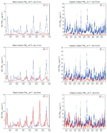
Over Mexico City (e.g. T0, T1), observed BC exhibits a strong diurnal variation (Yu et al., 2009), with the concentration increasing during the night and the largest values oc-curring in the morning hours around 08:00 LT. Because of the diurnal variation of PBL

20

depth and wind, the pollutants are trapped in the city overnight and during early morn-ing hours in a shallow surface layer before the rapid mixed layer growth commences in the morning. Comparing with observations over Mexico City (e.g. T0, Fig. 7), C3 captures the variation and maximum values of BC very well. C15 generally captures the observed variation of BC but significantly underestimates the magnitude during the

25

morning (06:00–10:00 LT). C75 fails to capture any peaks during entire week.

(18)

ACPD

10, 10777–10837, 2010

Y. Qian et al.

Title Page

Tables Figures

◭ ◮

Back Close

Full Screen / Esc

around 08:00 LT, since the PBL structure and evolution at T2 is similar with that at T1. Overall, the simulated BC concentration at T2 is 20–30% lower than at T1. Those features are consistent with the observations at T1 and T2 (Yu et al., 2009)

Organic Matter – The spatial distribution (not shown) and temporal variation (Fig. 7,

right panel) of OM are very similar with those for BC. This is not surprising since BC

5

and OM (excluding SOA in this study) share many common emission sources and their transport and mixing are often linked together (Hodzic et al., 2009). When comparing the three simulations against observations, the performance for OM is similar to BC (see Fig. 7 left panel). Transport from Mexico City to T2 appears to account for a substantial fraction of the BC and OM at T2. Since SOA is not included in the

WRF-10

Chem simulations, it is not surprising that simulated organic aerosol mass from all three simulations are lower than observed. Fast et al. (2009) and Hodzic et al. (2009) both show that simulated primary organic aerosols (POA) are similar to hydrocarbon-like organic aerosols (HOA) obtained via positive matrix factorization and Aerosol Mass Spectrometer (AMS) measurements.

15

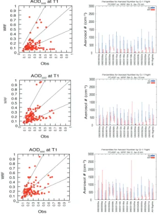
Aerosol Optical Depth– Figure 8 (left) shows scatter plots of AOD at 500 nm for the

observations at T1 versus the three simulations. The observed AOD ranges from 0.1 to 0.7, however, AOD simulated in C75 is below 0.3 for most cases, which is significantly underpredicted. C15 performs better than C75, with AOD ranging from 0 to 0.45. AOD simulated by C3 ranges from 0.05 to 0.95 and compares even better with

observa-20

tions. Recently, AERONET data have been widely used to evaluate or constrain AOD for global aerosol modeling and data assimilation (e.g. Dubovik et al. 2002). This study suggests that point measured AOD may reasonably represent the model grid cell av-erage if grid spacing is 3 km or smaller. When the grid resolution becomes larger, e.g. larger than 75 km, the model grid cell average may not correctly estimate AOD

mea-25

(19)

ACPD

10, 10777–10837, 2010

Y. Qian et al.

Title Page

Tables Figures

◭ ◮

Back Close

Full Screen / Esc

Aerosol Number Concentration – The aerosol number concentration, Na, is critical

information to investigate the indirect affect of aerosol on cloud and precipitation. The right column of Fig. 8 shows percentiles comparing observed (with a PCASP) and simulated Na for MOSAIC size bin 3 (0.15625 µm to 0.3125 µm dry particle diameter)

along the G-1 flight paths. C75 predicted Na, including median, percentile values and 5

ranges, are more than 2–3 times lower than observed for almost all the flights during the field campaign. C15 performs better at simulating Na, especially during the first half

of the month. Comparing C75 and C15 with C3 shows that C3 reasonably captures the median and percentile values of Na for most flights. All three simulations underpredict Na, possibly for many reasons. For example, SOA is not included which might impact 10

nucleation and there is uncertainty in the homogeneous nucleation parameterization. Also, uncertainties exist in the size distribution of emitted particles and some emission sources are missing, e.g. small biomass burning events, are not included in the emis-sion inventories used for this study. The underprediction of Na is much more serious

near the surface than aloft as measured by aircraft, especially for the simulation with

15

coarser resolution (not shown).

4 Sub-grid variability (SGV) of trace gases and aerosols

In this section we first present the probability density function (PDF) of trace gases and aerosols, and analyze the characteristics of their SGV, including the spatial distribution, diurnal and vertical variations, and dependences on the distance to emission sources

20

and the spatial resolution;

4.1 Definition of SGV

Each grid cell in C75 covers an area of 75×75 km2 (GC75) and contains a set of 5x5

(20)

ACPD

10, 10777–10837, 2010

Y. Qian et al.

Title Page Abstract Introduction Conclusions References Tables Figures ◭ ◮ ◭ ◮ Back Close

Full Screen / Esc

normalized standard deviation (SD) within a 75 km×75 km grid cell.

SGV= s 1 N N P

i₌1

(x_i₋x_¯₎2

¯

x

Here N=25 for C15 and N=625 for C3. xi refers to the value of a given species (e.g.

trace gas or particulate) for a C15 or C3 grid cell. ¯x_{is an average for the high resolution}

cells residing within the given C75 cell, GC75. This average consists of 25 C15 or 625

5

C3 grid cells for each GC75:

¯

x₌ 1 N

N

X

i₌1 x_i

Spatial variability is normalized by the average within GC75 so that the magnitude of SGV is not dependent on the species types or values. For a few variables, such as elevation, we also use standard deviation (SD) to describe their spatial variability.

10

S D₌

v u u t1 N N X

i₌1

(x_i₋x_¯₎

We calculate SGV or SD at every hour and make an average for entire valid simulation period from 5 to 30 March.

4.2 PDF

Figure 9 shows the frequency of occurrence of C3 simulated trace gases and aerosols

15

(21)

ACPD

10, 10777–10837, 2010

Y. Qian et al.

Title Page

Tables Figures

◭ ◮

Back Close

Full Screen / Esc

CO concentrations dramatically decreases, and maximum CO concentrations extends beyond 2.1 ppm only over regions close to emission sources. The maximum CO mixing ratio is 10 times larger than the minimum one, which is consistent with the observations and simulations in Tie et al. (2009).

O3 is distributed more evenly over a smaller range of values, i.e. the probabilities 5

are more similar across the O3concentration values and the maximum concentration

is around twice as large as the minimum one. The mixing ratio of O₃shows an approx-imately normal distribution. In contrast to CO, O3 is a secondary product with more

diverse sources and sinks and has a shorter lifetime. Similar to CO, the frequency of occurrences of BC dramatically decreases with the increase of concentration and

10

the maximum BC concentration is 9 times larger than the minimum one. Contrasting with BC are the properties of SO4, NO3, and NH4 (SNN), of which SO4 is the

domi-nant contributor by mass. SNN exhibit similar SGV properties with PDFs that are more evenly and narrowly distributed, and the maximum mixing ratio is around twice as large as the minimum one, although the frequency has an overall decreasing trend with the

15

increase of SNN mixing ratio.

In summary for the urban location, secondary trace gases and aerosols, such as O₃ and SNN, are more likely to have a normal distribution over a small range of values. For primary trace gases and aerosols, such as CO and BC, it is more likely to have a large range of values over polluted source regions, with the frequency decreasing with

20

increasing concentration.

For periods of southwesterly winds, T1, T2, T3, to T4 show the PDFs of the Mexico City plume as it is transported downwind. For other periods, the PDFs at these sites characterize the variability of trace gases and aerosols associated with high (T1) to low (T4) local emissions. For all periods, the PDFs from T1, T2, T3, and T4 gradually

be-25

come more evenly distributed for CO, BC, O₃and SNN. Over remote areas in general, all trace gases and aerosols are more evenly distributed compared to polluted areas.

(22)

ACPD

10, 10777–10837, 2010

Y. Qian et al.

Title Page

Tables Figures

◭ ◮

Back Close

Full Screen / Esc

falls between 2.5 and 5.0 m s−1 _{with a negative skew. RH has a positive skew with}

values typically between 40% and 50%. Maximum PBLH is two times higher than the minimum, which indicates a strong spatial variability of PBL structure over MC. The elevation varies from 2200 m to 3600 m, with around 30% of the area higher than 2500 m and a much larger amount of area with lower elevations.

5

4.3 Spatial pattern

Figure 10 shows the C3 spatial distribution of SGV for surface CO, BC, and SNN, and the SD for wind speed, PBLH, and terrain height. Maximum SGV for CO is centered over the MCMA, with a maximum value of 0.6–0.8. The spatial distribution of SGV for CO coincides with the maximum CO concentration (Fig. 5) and emission rates (Fig. 2),

10

even though SGV is normalized by the mean CO mixing ratio. This makes sense given that the strongest gradients in concentration typically exist where pollutants are emit-ted. High values exist in a grid cell containing emissions while non-emitting neighboring upwind cells can have very low concentrations in the most extreme case. Farther down-wind pollutants become more spatially mixed, and therefore more uniform with smaller

15

SGV. SGV for CO is smaller than 0.2 in other regions. Overall, the SGV for BC is larger than for CO, with a maximum value greater than 1.0 over Puebla (southeast of Mexico City), attributed to the higher emission and complex terrain along the southern border of the Mexican Plateau. The SGV of BC is larger than 0.3 over other remote regions, because of more widely spread emission sources (e.g. biomass burning) and larger

20

variability in surface concentrations of BC (Fig. 5).

SGV of SNN is larger than 0.2 over the majority of land areas, with a maximum value around 0.5 over Puebla. The SGV of SNN, with a range of 0.4 to 0.5, is much smaller than for BC and CO over the MCMA, which is consistent with the more evenly distributed PDF for SNN as shown in Fig. 9. This implies that the overall features

25

(23)

ACPD

10, 10777–10837, 2010

Y. Qian et al.

Title Page

Tables Figures

◭ ◮

Back Close

Full Screen / Esc

as seen in Fig. 10.

The SD for wind speed over land is around 1.0 to 1.6 m s−1 _{(Fig. 10), which is half}

of the mean wind speed at 10-m height. The SGV for wind speed is between 0.4 and 0.55 over the majority of the ocean (not shown). The SD for PBLH is between 140 and 280 m over land, with SGV around 0.4 to 0.65 (not shown). Maximum SD for elevation

5

is along the southern, eastern and northeastern borders of the Mexican Plateau, where T3 is located.

4.4 Vertical profile and diurnal variation of SGV

Figures 11 & 12 show the vertical profiles of SGV over the four GC75 for 6 variables during daytime and nighttime, respectively. During daytime (e.g. 15:00 LT as shown

10

in Fig. 11), the SGV for CO over T1 is around 0.6 within the PBL, i.e. below 2.75 km, but substantially drops to around 0.1 above the PBL top. The near vertically constant SGV within the PBL indicates that simulated CO is very efficiently transported and mixed vertically by turbulence but not well mixed horizontally, even in upper layers of the PBL. Indeed, the horizontal wind speed decreases only slightly with height and

15

vertical gradient of CO concentration is very small within the PBL (not shown). The nighttime vertical profile of CO, as shown at 03:00 LT in Fig. 12, is significantly different than during daytime. The SGV for CO over T1 reaches 0.8 at the surface, and quickly decreases with height. The shallower PBL and lower wind speed during nighttime does not facilitate the dispersion of pollutants vertically and horizontally, so the CO

20

mixing ratio is much larger at the surface during nighttime than during daytime. The CO concentration dramatically decreases in the free troposphere over T1 because of efficient horizontal transport, resulting in a significant decrease of CO SGV with height. The vertical variations of O₃SGV are similar to CO during both daytime and nighttime, except for a maximum SGV for O3observed in the lower stratosphere.

25

(24)

ACPD

10, 10777–10837, 2010

Y. Qian et al.

Title Page

Tables Figures

◭ ◮

Back Close

Full Screen / Esc

smaller below 1.5 km, which is similar as for CO. However, SGV for BC dramatically increases with height above 1.5 km and reaches a maximum value around the PBL top (around 3 km m.s.l.), which is not observed for CO. The vertical variability of SGV of CO is relatively straightforward within the PBL because CO concentration is mainly controlled by its emission rate and meteorological conditions. The concentration of BC

5

is also affected by deposition and interactions with other types of particles. An example of this type of interaction is the mixing of two different types of particulate species that have different spatial patterns for emissions. If only one of these species is present, there would be a given SGV, but when both species are present the SGV is modified, and typically increased, if the second specie has a different emission pattern. Because

10

MOSIAC uses an internal mixture for representing the particles, the net e_ffect is an increased SGV for particles compared to gases.

The vertical structure of SGV for SNN is very similar to BC during daytime over all four GC75, with a maximum SGV at the PBL top. During nighttime, however, the SGV is almost constant vertically with no large second peak as observed during daytime. The

15

different vertical variations of SGV for aerosols between daytime and nighttime within the PBL, where most of particulates are suspended, are important for estimating the SGV of direct radiative forcing of aerosol by reflecting and/or absorbing solar radiation during only daytime.

SGV of RH also exhibits double peaks in its vertical profile during daytime over T1

20

and T2 GC75, one at the surface and one at the PBL top. The vertical variability of SGV for RH is small and steady during nighttime over all four GC75. After being normalized by mean wind speed, the SGV for wind speed gradually decreases with height during nighttime. The SGV for wind speed during daytime is smaller at the surface and varies slightly vertically within the PBL.

25

(25)

ACPD

10, 10777–10837, 2010

Y. Qian et al.

Title Page

Tables Figures

◭ ◮

Back Close

Full Screen / Esc

and the particulate species. Animations of all the RH profiles contributing to a given GC75 (not shown) reveal that the RH typically is highest at the top of the PBL and then strongly decays above the PBL. Because the PBL height is not constant within a given GC75, small changes in the PBL height cause a strong gradient in RH leading to large SGV. At night when the PBL decays, the RH typically peaks near the surface and the

5

peak aloft goes away.

It should be noted that there is a strong relationship between the SGV vertical profile for RH and the particulates. Close examination of Figs. 11 and 12 reveal that the existence of the SGV peak at the top of the PBL typically correspond between RH, BC, and SNN. All of these tend to form or not form peaks consistently at the same time of

10

day and locations. For example, in the nighttime profile for T3 the RH maintains the SGV peak similar to during the daytime and the aerosol SGV also maintains the peak aloft at night. There are mechanisms that connect RH to aerosol processes such as particle coagulation and chemical reaction rates. So, the RH SGV likely directly impacts the particulate SGV. However, since the particulates also have a strong gradient at the

15

top of the PBL, the undulating PBL most likely plays a larger role in establishing the SGV peak at the PBL top than the RH interactions.

Figure 13 shows the diurnal cycle of SGV at the surface. SGV of CO exhibits two peaks over T1. The first peak with maximum SGV of 1.2 occurs at 07:00 LT when the CO concentration peaks and the PBL starts growing. The second SGV peak of

20

about 1.0 occurs around midnight. The diurnal variation pattern of SGV for CO shown in Fig. 12 is consistent with that for CO concentration (not shown), but it should be remembered that SGV is normalized by mean CO concentration. While CO concen-tration during nighttime is larger than during daytime, it exhibits a noticeable minimum around 03:00 LT. In theory, the CO concentration should continuously increase from

25

(26)

ACPD

10, 10777–10837, 2010

Y. Qian et al.

Title Page

Tables Figures

◭ ◮

Back Close

Full Screen / Esc

O₃, which has higher concentrations during daytime and lower concentrations during nighttime, exhibits an opposite diurnal cycle compared to CO. However, SGV for O3

shows a similar diurnal cycle to CO, except for a smaller magnitude, with one peak around 07 LT and another around midnight over T1 GC75. SGV for BC is larger during nighttime than during daytime, with one SGV peak of 1.1 around 07:00 LT. The SGV for

5

BC exhibits a different diurnal variation compared to CO, although the concentration of BC has a very similar diurnal cycle as CO, with a low values around 03 affected by lower BC emission between 00 and 06:00 LT. The maximum SGV for SNN occurs in early afternoon with a magnitude around 0.75, smaller than CO, O3, or BC. The SGV

for RH is around 0.2 and a maximum value occurs later in the afternoon that is less

10

than 0.4, which is smaller than SGV for trace gases and aerosols. The SGV for wind speed reaches a maximum (above 0.7 for T1) around early morning over all GC75, which partly contributes to the maximum SGV for trace gases and aerosols around 07:00 LT.

4.5 Dependences of SGV on the distance to the polluted sources

15

Figures 11–13 also can be interpreted as vertical profiles and diurnal variations of SGV for increasing distance from the large urban emission source as once progresses from T1 to T2, T3, and T4. The vertical and diurnal variations over T1 GC75 are described in Sect. 4.4. Here the discussion focuses on the differences of SGV among the four areas.

20

The vertical variation of CO and O₃ over T2 is similar with that over T1 during both daytime and nighttime, but with a smaller magnitude of SGV within the PBL over T2, especially at the surface during nighttime. For example, within the PBL, the SGV for both CO and O₃ over T2 is nearly constant vertically during daytime but at night de-creases quickly with distance above the surface, which is consistent with T1. But the

25

SGV for CO and O3 at T2 is 30–40% as large as at T1 during daytime, resulting from

(27)

ACPD

10, 10777–10837, 2010

Y. Qian et al.

Title Page

Tables Figures

◭ ◮

Back Close

Full Screen / Esc

The vertical profile of SGV for BC and SNN over T2 is similar as over T1 and a SGV peak also appears at the PBL top during daytime, except with a smaller magnitude over T2. A SGV peak also appears at the PBL top over T3 in both daytime and nighttime, but vertical variability of SGV is smaller over T4. Generally, the SGV for BC and SNN are larger than for CO and O3 because of larger and more variable emissions of BC 5

and SNN precursors over rural or remote areas. For RH and wind speed, SGV over T2 exhibits similar vertical pattern as over T1, but with a smaller magnitude at T2 during daytime. Overall SGV for RH and wind speed does not differ as much over the four GC75 as for trace gases and aerosols because the spatial variability of meteorological variables does not depend on local emission rates.

10

The vertical profiles show that major di_fferences in SGV among the four GC75 occur within the PBL, especially near the surface. Figure 13 compares the daily mean SGV over the four GC75 at the lowest model level, which reflects the state of the entire PBL for CO and O₃. Surface SGV of CO at T1 is about two times larger than at T2 and 10 times larger than at T3 and T4. Surface SGV of O3at T1 is about two and three times 15

as large as at T2 and at T3 and T4, respectively. SGV of BC and SNN over T2, T3, and T4 are smaller during daytime because of more e_fficient ventilation, are larger during nighttime, and do not have the two diurnal peaks. This is different than at T1 where two peaks exist at midnight and 07:00 LT. The SGV for BC and SNN are larger at T1 than at the other three GC75, but the di_fference between urban and downwind remote

20

regions is much smaller than for CO and O3. For BC and SNN, the difference of SGV

is very small among T2, T3, and T4.

As summarized in Fig. 14, the SGV for trace gases and aerosols generally decreases with the distance away from the urban area with large emission sources, even with the normalization by the mean concentrations. As described in Sect. 2.2, the model lateral

25

boundaries provide time dependent inflow conditions for pollutants from other portions of the globe, which is important for species with longer chemical life times, e.g. CO and O3. Aerosols and short-lived trace gases over T3 and T4 are not likely to be affected

(28)

ACPD

10, 10777–10837, 2010

Y. Qian et al.

Title Page

Tables Figures

◭ ◮

Back Close

Full Screen / Esc

Our simulations show that the decreasing rate of SGV with the distance is more significant for trace gases than for aerosols. Among the trace gases, the decrease of SGV with distance for CO is more dramatic than for O3, while among the aerosols the

decrease of SGV with distance for BC is more dramatic than for SNN. This implies that the SGV primary trace gases and aerosols with a longer lifetime decrease with distance

5

more quickly than for secondary trace gases and aerosols. This is probably related to the emission source, whether it is more localized or more wide-spread spatially, and the interaction and deposition processes of aerosols species. In addition, the rate at which SGV decreases with the distance away from the polluted urban area is more significant during daytime than at nighttime.

10

4.6 Dependences of SGV on the spatial resolution

Figure 14 also compares SGV for trace gases and aerosols over the four GC75 be-tween two simulations with 3-km and 15-km grid spacing (i.e. C3 and C15), respec-tively. The SGV for CO, BC and SNN are 60-100% larger for C3 than for C15 over the T1 urban site, even though the SGV of emissions is only 25–35% larger at C3

15

compared to C15 over the same grid cell (Fig. 15). Over the other GC75 (i.e. T2, T3, and T4), the SGV for trace gases and aerosols are 30–60% larger for C3 than for C15, except for CO, which has a much lower SGV over these rural or remote areas. For me-teorological variables, the SGV is 20-30% larger in C3 than in C15 for RH and PBLH and 20–60% larger for wind speed over the four GC75. The increase of SGV from

20

C15 to C3, ranging from 150% over T1 to 60% over T3 (Fig. 15), is much larger for cloud optical depth than for other meteorological variables. Overall, the SGV for C3 is larger than for C15 for all variables, which numerically implies that the model solution has not converged at the 3-km grid spacing. However, it is unreasonable to expect full convergence, i.e. the result does not change with a further increase in resolution,

25

(29)

ACPD

10, 10777–10837, 2010

Y. Qian et al.

Title Page

Tables Figures

◭ ◮

Back Close

Full Screen / Esc

from clouds, topography, etc. that get introduced as the resolution increases. Most importantly, the increase of SGV for trace gases and aerosols is stronger than for most meteorological variables. This sensitivity is most likely due to the increased SGV of emissions at higher resolutions.

5 Impacts of emission and terrain on the SGV of trace gases and aerosols

5

In Sect. 4 we discussed the spatial and temporal variations of SGV for trace gases, aerosols, and meteorological variables. However, what factors affect the subgrid pro-cessing and variability of trace gases and aerosols, and how significant are each of those factors? In this section we discuss the contributions of emissions and orography on the SGV based on the results of sensitivity experiments.

10

5.1 Emissions

It would be expected that the spatial variability of emissions has a great impact on the SGV of trace gases and aerosols over urban areas. Figure 16 shows the vertical profiles of 24-hour mean SGV over T1 for three simulations with 15-km grid spacing. The settings for E15 are exactly same as for C15, except that the emission rates in

15

E15 are averaged to match the emissions from the 75-km grid. In effect, this makes the emission values constant for each 5×5 set of grid cells in E15, corresponding to

the single 75-km grid cell from C75. So, the di_fference between output from C15 and E15 reflects the contribution of emission spatial variability between global model and regional model grid spacings on the SGV of trace gases and aerosols.

20

As shown in Fig. 16, the vertical profile of SGV for C15 is similar to the profile for C3 over T1 when we combine the day and nighttime profiles in Figs. 11 and 12, except for a smaller magnitude in C15 as discussed in Sect. 4.6. With a uniform emission rate used in T1 GC75 (i.e. E15), the SGV decreases from 0.38 to 0.21 for CO and from 0.34 to 0.18 for BC at the surface during daytime (not shown). The differences of SGV

(30)

ACPD

10, 10777–10837, 2010

Y. Qian et al.

Title Page

Tables Figures

◭ ◮

Back Close

Full Screen / Esc

(15–25%) between C15 and E15, however, are much smaller during nighttime over T1, partly because of the minimum emissions rate after midnight (see Sect. 4.4). As shown in Fig. 16, the daily averaged SGV difference between E15 and C15 is around 37% for CO and BC at the surface, and decreases with height in the PBL.

Differences in SGV between C15 and E15 for O3 and SNN decrease with height 5

within the PBL during daytime (not shown) and are smaller than for CO and BC. When uniform emissions are used in each GC75, the SGV drops by 25% for O₃and by 15% for SNN during daytime. The changes in SGV are minor for O3 and SNN during the

night. The daily averaged SGV changes are 10–20% for O3 and SNN at the surface

(Fig. 16). The differences of SGV between C15 and E15 are near zero in the free

10

troposphere for trace gases, aerosols, and meteorological variables. The SGV for meteorological variables, including RH and wind, are not affected by the emission rates in the simulations since there is minimal feedback between aerosols and meteorology in the chosen model configuration, only the aerosol direct e_ffect.

The impact of emissions on SGV of trace gases and aerosols is much less significant

15

over rural or remote areas. As shown in Fig. 17, the SGV differences are almost indistinguishable over T3, except for near the surface where SGV actually increases in E15 for CO, BC, and SNN. However, both the emission amount and the SGV are small over T3. At T3, which has complex and varied terrain, the SGV for trace gases and aerosols is primarily determined by terrain rather than by emissions.

20

In summary, the spatial variability of emissions can account for up to 50% of the SGV during daytime for long-lived trace gases and aerosols, such as CO and BC, over urban areas like MC. The impact of emissions on secondary trace gases and aerosols, such as O3 and SNN, are less than for CO and BC. The impact of emissions on the SGV

of trace gases and aerosols decays with altitude in the PBL and has almost no effect

25