Simulation of trace gases and aerosols over the Indian domain: evaluation of the WRF-Chem model

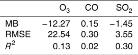
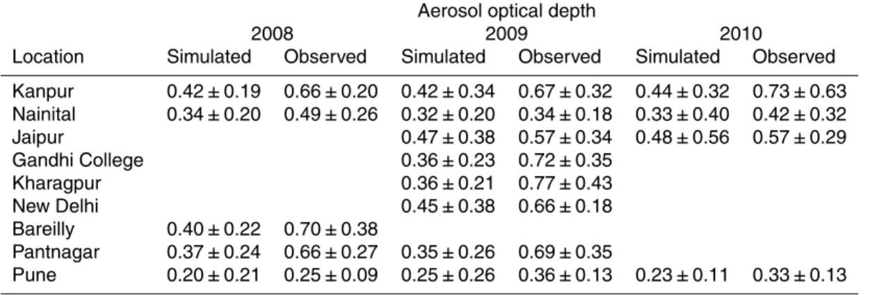
Therefore, the objectives of this work are (i) to assess whether the inclusion of aerosol radiative feedbacks in the online coupled WRF-Chem model improves the modelling outputs

Examples of the elevated layers observed for ozone and various other trace gases and aerosol properties during INDOEX: (A) O 3 profiles over KCO from balloon sondes (solid line)

Measurements of aerosol chemical composition and aerosol optical depth in the Nepal Himalaya have clearly shown the build up of aerosols in the pre-monsoon season during the winter

These measurements are used to retrieve spatially resolved information of the stratospheric aerosol distribution, including spectral extinction coe ffi cient and particle size.. Here

during the 2006 MILAGRO field campaign using multiple spatial resolutions and sce- narios that examine SGV of emissions and terrain. Our analysis focuses on quantifying the SGV of

Using Pollution Load Index and Geo-accumulation Index for the Assessment of Heavy Metal Pollution and Sediment Quality of the Benin River, Nigeria. Heavy metals

At the first stage of the measurements results analysis, the gear wheel cast surface image was compared with the casting mould 3D-CAD model (fig.. Next, the measurements results

The structure of the remelting zone of the steel C90 steel be- fore conventional tempering consitute cells, dendritic cells, sur- rounded with the cementite, inside of

References

Ackermann, I. J., Hass, H., Memmesheimer, M., Ebel, A., Binkowski, F. S., and Shankar, U.: Modal aerosol dynamics model for Europe: development and first applications, Atmos. Envi-ron., 32, 2981–2999, doi:10.1016/S1352-2310(98)00006-5, 1998.
Adhikary, B., Carmichael, G. R., Tang, Y., Leung, L. R., Qian, Y., Schauer, J. J., Stone, E. A., 5
Ramanathan, V., and Ramana, M. V.: Characterization of the seasonal cycle of south Asian aerosols: a regional-scale modeling analysis, J. Geophys. Res., 112, D22S22, doi:10.1029/2006JD008143, 2007.
Anderson, T. L., Charlson, R. J., Bellouin, N., Boucher, O., Chin, M., Christopher, S. A., Hay-wood, J., Kaufman, Y. J., Kinne, S., Ogren, J. A., Remer, L. A., Takemura, T., Tanré, D., 10
Torres, O., Trepte, C. R., Wielicki, B. A., Winker, D. M., and Yu, H.: An “A-Train” strategy for quantifying direct climate forcing by anthropogenic aerosols, B. Am. Meteorol. Soc., 86, 1795–1809, doi:10.1175/BAMS-86-12-1795, 2005.
Bian, H., Tie, X., Cao, J., Ying, Z., Han, S., and Xue, Y.: Analysis of a severe dust storm event over China: application of the WRF-Dust model, Aerosol Air Qual. Res., 11, 419–428, 15
doi:10.4209/aaqr.2011.04.0053, 2011.
Carmichael, G. A., Adhikary, B., Kulkarni, S., D’Allura, A., and Tang, Y.: Asian aerosols: current and year 2030 distributions and implications to human health and regional climate change, Environ. Sci. Technol., 43, 5811–5817, doi:10.1021/es8036803, 2009.
Chen, F. and Dudhia, J.: Coupling an advanced land surface–hydrology model with the Penn 20
State-NCAR MM5 modeling system – Part 1: Model implementation and sensitivity, Mon. Weather Rev., 129, 569–585, doi:10.1175/1520-0493(2001)129<0569:CAALSH>2.0.CO;2, 2001
Cherian, R., Venkataraman, C., Ramachandran, S., Quaas, J., and Kedia, S.: Examination of
aerosol distributions and radiative effects over the Bay of Bengal and the Arabian Sea region
25
during ICARB using satellite data and a general circulation model, Atmos. Chem. Phys., 12, 1287–1305, doi:10.5194/acp-12-1287-2012, 2012.
Cherian, R., Venkataraman, C., Quaas, J., and Ramachandran, S.: General circulation model (ECHAM5-HAM) studies of aerosol extinction, atmospheric heating and precipitation pat-terns over India, J. Geophys. Res., submitted, 2014.
30
(24)
gen-GMDD
7, 431–482, 2014
Evaluation of the WRF-Chem model
M. Michael et al.
Title Page
Abstract Introduction
Conclusions References
Tables Figures
◭ ◮
Back Close
Full Screen / Esc
Printer-friendly Version Interactive Discussion