Hydrol. Earth Syst. Sci., 17, 2685–2699, 2013 www.hydrol-earth-syst-sci.net/17/2685/2013/ doi:10.5194/hess-17-2685-2013
© Author(s) 2013. CC Attribution 3.0 License.
Geoscientiic
Geoscientiic
Hydrology and
Earth System
Sciences
Open Access
Regionalization of patterns of flow intermittence from gauging
station records
T. H. Snelder1,2, T. Datry1, N. Lamouroux1, S. T. Larned3, E. Sauquet4, H. Pella1, and C. Catalogne4
1IRSTEA, UR MALY, Lyon, France
2Aqualinc Research, Christchurch, New Zealand
3National Institute of Water and Atmospheric Research, Christchurch, New Zealand 4IRSTEA, UR HHLY, Lyon, France
Correspondence to:T. H. Snelder ([email protected])
Received: 24 December 2012 – Published in Hydrol. Earth Syst. Sci. Discuss.: 30 January 2013 Revised: 20 May 2013 – Accepted: 1 June 2013 – Published: 11 July 2013
Abstract.Understanding large-scale patterns in flow inter-mittence is important for effective river management. The duration and frequency of zero-flow periods are associated with the ecological characteristics of rivers and have impor-tant implications for water resources management. We used daily flow records from 628 gauging stations on rivers with minimally modified flows distributed throughout France to predict regional patterns of flow intermittence. For each sta-tion we calculated two annual times series describing flow intermittence; the frequency of zero-flow periods (consec-utive days of zero flow) in each year of record (FREQ; yr−1), and the total number of zero-flow days in each year
of record (DUR; days). These time series were used to cal-culate two indices for each station, the mean annual fre-quency of zero-flow periods (mFREQ; yr−1), and the mean
duration of zero-flow periods (mDUR; days). Approximately 20 % of stations had recorded at least one zero-flow pe-riod in their record. Dissimilarities between pairs of gauges calculated from the annual times series (FREQ and DUR) and geographic distances were weakly correlated, indicating that there was little spatial synchronization of zero flow. A flow-regime classification for the gauging stations discrim-inated intermittent and perennial stations, and an intermit-tence classification grouped intermittent stations into three classes based on the values of mFREQ and mDUR. We used random forest (RF) models to relate the flow-regime and in-termittence classifications to several environmental charac-teristics of the gauging station catchments. The RF model of the flow-regime classification had a cross-validated Cohen’s kappa of 0.47, indicating fair performance and the
intermit-tence classification had poor performance (cross-validated Cohen’s kappa of 0.35). Both classification models iden-tified significant environment-intermittence associations, in particular with regional-scale climate patterns and also catch-ment area, shape and slope. However, we suggest that the fair-to-poor performance of the classification models is be-cause intermittence is also controlled by processes operat-ing at scales smaller catchments, such as groundwater-table fluctuations and seepage through permeable channels. We suggest that high spatial heterogeneity in these small-scale processes partly explains the low spatial synchronization of zero flows. While 20 % of gauges were classified as inter-mittent, the flow-regime model predicted 39 % of all river segments to be intermittent, indicating that the gauging sta-tion network under-represents intermittent river segments in France. Predictions of regional patterns in flow intermittence provide useful information for applications including envi-ronmental flow setting, estimating assimilative capacity for contaminants, designing bio-monitoring programs and mak-ing preliminary predictions of the effects of climate change on flow intermittence.
1 Introduction
(Lake, 2003) (Turner and Richter, 2011). Many river net-works in arid regions are entirely intermittent (Jacobson and Jacobson, 2013; Meirovich et al., 1998). Temporal patterns of flow intermittence range from near-perennial flow regimes with infrequent, short periods of zero flow to episodic flow regimes with rare flow events separated by long zero-flow periods (Crocker et al., 2003; Houston, 2006; Larned et al., 2011; Meirovich et al., 1998). In turn, the duration and fre-quency of zero-flow periods are increasingly viewed as the primary determinants of river ecosystem processes (Corti et al., 2011; Datry et al., 2011; Dieter et al., 2011) and biotic communities (Arscott et al., 2010; Datry, 2012; Davey and Kelly, 2007).
Many intermittent rivers support diverse plant and ani-mal communities, particularly when viewed at timescales that encompass periods of river flow, standing water, and no water. Aquatic and terrestrial species colonize and emi-grate from intermittent rivers in response to shifts between wet and dry habitat (Acu˜na et al., 2005; Corti and Datry, 2012; Datry et al., 2012; Davey and Kelly, 2007; Steward et al., 2011). A smaller number of intermittent river specialists persist through multiple wet–dry cycles; this group includes aestivating fish and encysting invertebrates (Kikawada et al., 2005; Perry et al., 2008; Sayer, 2005). The alternating oc-cupation of habitat by aquatic and terrestrial species means that the time-averaged biodiversity of intermittent segments can exceed that of perennial segments (Katz et al., 2012). In addition to their ecological values, intermittent rivers pro-vide numerous ecosystem services, including flood irriga-tion, flood control, and waste-water conveyance (Angel et al., 2010; Larned et al., 2010a). In the Mediterranean region and other water-scarce areas, intermittent rivers represent an im-portant source or the sole source of freshwater for human use (e.g., Jacobson and Jacobson, 2013; Ji et al., 2006). Under-standing large-scale patterns in flow intermittence in these regions is a prerequisite for effective water resources man-agement.
The last decade has seen rapid growth in ecological and water resources research focused on intermittent rivers (Da-try et al., 2011). This research has been accompanied by a widespread acknowledgment that intermittent rivers re-quire careful management to protect biological and socio-economic values (Jacobson and Jacobson, 2013; Larned et al., 2010a; Nadeau and Rains, 2007). However, current man-agement practices and natural resources policies are often inadequate. For example, there are fewer restrictions im-posed on the use or alteration of intermittent rivers in the United States compared with perennial rivers (Leibowitz et al., 2008). In much of the world, alterations of intermittent river channels and flow regimes are entirely unrestricted (El-more and Kaushal, 2008; G´omez et al., 2005; Hughes, 2005). Effective management of intermittent rivers is impeded by the scarcity of information about their abundance, distribu-tion patterns, patterns of flow variability, and the
environ-mental conditions that produce those patterns (Datry et al., 2011; Fritz et al., 2008; Hansen, 2001).
Identifying intermittent rivers and river segments, and characterizing intermittent flow regimes at scales larger than individual catchments pose several challenges. Small-scale river maps (>1 : 25 000) produced from digital elevation models, aerial photography or airborne laser scanning omit many intermittent segments (Hansen, 2001; Leopold, 1994). More intermittent segments are included in detailed maps based on field surveys (e.g., Brooks and Colburn, 2011), but large-scale field surveys are prohibitively laborious. As alternatives to surveys and remote sensing, empirical mod-els have been used to predict the locations of intermittent river segments based on catchment characteristics (Bent and Steeves, 2006; Heine et al., 2004; Wood et al., 2009). These models perform moderately well in the areas for which they are defined and provide information about intermittence-environment associations over large, intermittence-environmentally hetero-geneous areas. For example, an empirical model used to pre-dict the occurrence of streams identified as intermittent or perennial based on visual observation during low-flow peri-ods in the state of Massachusetts was reasonably accurate, with a misclassification rate of approximately 20 %, (Bent et al., 2006). In another empirical modeling study, intermittent segments in forested headwater streams were distinguished from perennial segments using field survey data (Fritz et al., 2008). However, survey data alone are insufficient for further subdividing intermittent segments on the basis of intermittent flow patterns (i.e., grouping segments with similar frequen-cies and durations of zero flow); this step requires flow time series that field surveys cannot provide.
Grouping gauging stations into flow-regime classes based on time-series data is an important component of large-scale river management and research (Olden et al., 2012). Flow-regime classifications serve as spatial frameworks for envi-ronmental monitoring, and they simplify water allocation de-cisions and environmental flow setting (Kennard et al., 2010; Olden et al., 2012; Snelder et al., 2009). Most flow-regime classifications are based on hydrological indices calculated from time series recorded at gauging stations. Hydrologi-cal indices describe the magnitude, timing, duration, rate-of-change and frequency of flow events. Statistical similar-ities in hydrological indices are then used to group gaug-ing stations with similar flow regimes (Olden et al., 2012). The utility of a flow-regime classification is maximized when class membership can be extrapolated to ungauged loca-tions. In several recent studies, flow time series have been combined with spatial data describing environmental con-ditions in statistical classifications that were used to pre-dict river flow regimes at ungauged locations (e.g., Kennard et al., 2010; Snelder et al., 2009). To our knowledge, there have been no comparable studies that focused specifically on flow intermittence.
modified flows regimes to study regional patterns of flow intermittence. Our study had two objectives: (1) to charac-terize flow intermittence in terms of the spatial distribution of intermittent segments, and the frequency and duration of zero-flow periods in those segments; and (2) to determine the extent to which flow intermittence patterns are associated with environmental conditions.
2 Materials and methods 2.1 Study area
The study area was continental France, which extends from 42◦19′to 51◦5′N latitude and from 4◦46′W to 8◦14′E
lon-gitude and has an area of 550 000 km2. Environmental varia-tion within France that is pertinent to hydrological patterns is summarized by the hydro-ecoregions (HER) framework (Wasson et al., 2002). The HER is a regionalization de-veloped for river management in accordance with the Eu-ropean Water Framework Directive. The first level of the HER divides France into 21 regions based primarily on vari-ation in climate, topography and geology. Climate condi-tions in the hydro-ecoregions range from mediterranean in the “M´editerran´een” and “C´evennes” regions to temperate maritime in the “Armoricain” region, to cold and wet in the Alpine “Alpes internes” (Fig. 1). Geological conditions range from calcareous in the “Jura-Pr´ealpes” regions to alluvial in the “Plaine Saˆone” and “Alsace” regions (Fig. 1). Topo-graphic conditions range from plains in the “Alsace” regions to high mountains in the “Alpes internes” and “Pyr´en´eees” regions.
2.2 Hydrological data
We started our analysis with a hydrology dataset composed of time series of daily mean flow from over 3800 gaug-ing stations distributed throughout France, acquired from the HYDRO database (http://www.hydro.eaufrance.fr/). We re-moved stations from the dataset that lacked quality-assured data as defined by the HYDRO database managers, and for which the flow records were coded as modified due to the presence of reservoirs, diversions or significant abstractions in the upstream catchment. From the remaining stations, we selected those for which flow data were available in the 35 yr period from 1975 to 2009. We searched these records for gaps longer than 20 days and removed the year of record in which these gaps occurred. This resulted in an average re-moval of 1.2 (std dev = 1.7) yr per station. After these steps, 628 stations with 23–35 yr of record were retained (Fig. 2).
2.3 Flow variables and indices
We used the daily flow data for each gauging station to pro-duce two annual times series describing flow intermittence; the frequency of zero-flow periods (consecutive days of zero
Fig. 1. France showing the hydro-ecoregion (HER) boundaries (Wasson et al., 2002). The number of gauging stations included in this study in each region is shown in parentheses in the legend.
flow) in each calendar year of record (FREQ; yr−1), and
the total number of zero-flow days in each calendar year of record (DUR; days). From these time series we calcu-lated two inter-annual indices for each station, the mean an-nual frequency of zero-flow periods (mFREQ; yr−1), and the
mean duration of zero-flow periods (mDUR; days). To de-termine whether zero flows may have been recorded at some gauging stations due to freezing, we also calculated mFREQ and mDUR separately for the winter season, December to February.
2.4 River network and environmental variables
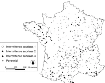
Fig. 2.Map of the location of the gauging stations used in this study. Stations on perennial segments are indicated by closed circles. Sta-tions on intermittent segments are classified into three intermittence subclasses (see text for class descriptions).
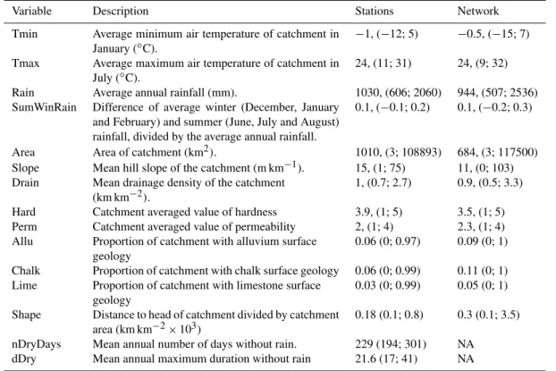
Rainfall and air temperatures were measured by M´et´eo-France at meteorological stations during the period 1961– 1990 and were interpolated onto a 1 km grid (resolution 1 km) using the method of Benichou and Le Breton (1987). The climatic layers included average annual rainfall, mean monthly rainfall, average maximum daily temperature in the warmest month (July) and average minimum daily temper-ature in the coldest month (January). The tempertemper-ature and rainfall data were then used to calculate values of the fol-lowing variables for the catchment of each segment: average annual rainfall (Rain), the difference between average sum-mer and winter rainfall divided by annual average rainfall (SumWinRain), average minimum January air temperature (Tmin), and average maximum July air temperature (Tmax) (Table 1). We derived two additional climate variables that described periods without rainfall: the catchment average of the mean annual number of days without rain (nDryDays), and the catchment average of the mean annual maximum duration of consecutive days without rain (dDry). The data used for these predictors were available only for stations, not for the entire network. Values of nDryDays and dDry were obtained from a rainfall time series for the period 1970 to 2005 generated for the catchment of each gauging station de-rived from the high-resolution Safran atmospheric reanalysis over France (Quintana-Segu´ı et al., 2008) using methods de-scribed by Sauquet and Catalogne (2011).
Topographic data consisted of a slope grid that we de-rived from the DEM, and mapped river channels represented on the 1 : 250 000 scale BD Carthage® map obtained from IGN. We used the river-channel map to derive an estimate of the observed drainage density that was independent of our DEM-based network. We considered that the observed
net-work density may reflect relevant soil and geological charac-teristics such as perviousness of the surficial material and that this may provide a useful predictor variable. We calculated the catchment average values of slope and drainage density for each segment to define the variables Slope and Drain (Ta-ble 1). We also used the DEM to estimate the distance from each segment to the most distant point of its upstream catch-ment. This distance divided by catchment area was defined as the variable Shape. Elongated catchments have high val-ues of Shape, and round catchments have low valval-ues.
Geological data were derived from a 1 :1 000 000-scale digital geological map of France obtained from Bureau des Recherches G´eologiques et Mini`eres (BRGM, 1996). The map defined 22 categories and comprised approximately 18 000 individually categorized polygons with a mean area of 40 km2. The map was used to develop two GIS layers de-scribing physical hardness (i.e., resistance to erosion) and permeability. For each layer, each of the 22 geological cat-egories was assigned an ordinal value corresponding to rela-tive hardness and permeability (Table 2). For detailed meth-ods, see Snelder et al. (2008). We computed the catchment surface area weighted mean of the ordinal values represent-ing physical hardness (Hard) and permeability (Perm) of geo-logical categories. We also computed the proportions of each catchment occupied by the broad geological categories chalk (Chalk), limestone (Lime) and alluvium (Alluv) (Table 2). We also derived the average segment subcatchment values of the ordinal values representing hardness and permeability (segHard and segPerm) and the geological categories chalk (segChalk, segLime and segAlluv) to address the possibility that local geological conditions affect flow intermittence.
2.5 Flow regime and intermittence classifications
Table 1.Regionalization of patterns of flow intermittence from gauging station records.
Variable Description Stations Network
Tmin Average minimum air temperature of catchment in
January (◦C). −
1, (−12; 5) −0.5, (−15; 7)
Tmax Average maximum air temperature of catchment in July (◦C).
24, (11; 31) 24, (9; 32)
Rain Average annual rainfall (mm). 1030, (606; 2060) 944, (507; 2536) SumWinRain Difference of average winter (December, January
and February) and summer (June, July and August) rainfall, divided by the average annual rainfall.
0.1, (−0.1; 0.2) 0.1, (−0.2; 0.3)
Area Area of catchment (km2). 1010, (3; 108893) 684, (3; 117500) Slope Mean hill slope of the catchment (m km−1). 15, (1; 75) 11, (0; 103)
Drain Mean drainage density of the catchment (km km−2).
1, (0.7; 2.7) 0.9, (0.5; 3.3)
Hard Catchment averaged value of hardness 3.9, (1; 5) 3.5, (1; 5) Perm Catchment averaged value of permeability 2, (1; 4) 2.3, (1; 4) Allu Proportion of catchment with alluvium surface
geology
0.06 (0; 0.97) 0.09 (0; 1)
Chalk Proportion of catchment with chalk surface geology 0.06 (0; 0.99) 0.11 (0; 1) Lime Proportion of catchment with limestone surface
geology
0.03 (0; 0.99) 0.05 (0; 1)
Shape Distance to head of catchment divided by catchment area (km km−2
×103)
0.18 (0.1; 0.8) 0.3 (0.1; 3.5)
nDryDays Mean annual number of days without rain. 229 (194; 301) NA dDry Mean annual maximum duration without rain 21.6 (17; 41) NA
2.6 Spatial synchronization of intermittence patterns
To better understand the spatial scale of observed intermit-tence patterns, we evaluated the degree of spatial synchro-nization of the variables FREQ and DUR at the gauging sta-tions on intermittent segments using the Mantel statisticr
(Mantel, 1967). The Mantel statistic is the Pearson correla-tion coefficient between two matrices of dissimilarities and is used to quantify spatio-temporal clustering (i.e., spatially organized synchronization). Our first matrix described the dissimilarity in annual intermittence patterns between pairs of stations. Our second dissimilarity matrix defined the geo-graphic (Euclidian) distance between pairs of stations. The significance of the statistic is established by permutation based on the null hypothesis of “no correlation” (Legendre and Legendre, 1998). The procedure made random permu-tations of the rows in one matrix and recomputed the corre-lation. The observed correlation was compared to the distri-bution of values derived from 10 000 permutations and mea-sures the probability of obtaining higher than observed cor-relation by chance (Legendre and Legendre, 1998).
Dissimilarities in the two annual times series describing flow intermittence (FREQ and DUR) between pairs of sta-tions were calculated as (1−ρ), whereρis the rank (Spear-man) correlation of the time series. Therefore, stations were compared on the basis of the relative frequency and duration of zero flow in each year, rather than the absolute magnitudes of the events. The calculation of dissimilarities was
compli-cated by missing data for some years as a result of gaps or because the station records had differing durations within the analysis period. Thus, we calculated the correlation between each pair of stations for the years in which data were avail-able at both stations.
The assumption of linearity is implicit in Mantel tests and consequently, the tests will not detect spatial structures if there are non-linear relationships between space and syn-chronous behavior. For example, gauging stations in close proximity may have similar temporal behavior, but the be-havior of widely separated pairs of stations may be unre-lated. We used a Mantel correlogram to determine the level of synchrony among the gauging stations at different spatial scales (Goslee and Urban, 2007). The Mantel correlogram used Mantel tests to determine the correlations between geo-graphic distance and the indices FREQ and DUR for subsets of stations belonging to several distance classes. The dis-tance classes subdivided the log-transformed disdis-tances be-tween stations into nine equi-distant categories. Because of the multiple comparisons made by the Mantel correlogram, Bonferroni corrections were applied before interpreting the significance of the correlations (Goslee and Urban, 2007).
2.7 Statistical modeling of classifications
Table 2.Geological categories represented on the 1 : 1 000 000 scale geological map of France (BRGM, 1996). Ordinal values of physi-cal hardness range from 1 (soft) to 5 (hard); ordinal values of per-meability range from 1 (impermeable) to 4 (permeable). The fourth column shows the geological categories that were also included in-dependently as environmental variables in our analysis (as propor-tion of the catchment in category). The sum of three categories was used to define alluvium (Allu).
Catchment Geological Physical geological category hardness Permeability category
Fluvial alluvium 1 3 Allu Quaternary alluvium 1 3 Allu Clay and sand 1 1
Limestone 5 4 Lime
Chalk 3 4 Chalk
Glacial deposit 1 1 Sedimentary flysch 3 2
Marls 3 1
Marls with evaporates 3 1
Molasse 2 3
Basaltic rock 5 1 Igneous rock 5 1 Calcareous detrial rock 4 2 Cystaline detrial rocks 5 1 Noncalcareous detrial rock 5 3 Metamorphic rocks 5 1 Volcanic rocks 5 2
Sand 1 3 Allu
Carbonaceous schist 3 2 Metamorphic schist 3 2 Sedimentary schist 3 2 Stratified calcareous rocks 3 2
gauging stations on the basis of flow-regime class (peren-nial and intermittent) using the environmental variables as predictors. The statistical model was used to assess the de-gree to which intermittence was related to different environ-mental variables, and to make predictions of the flow-regime class for all segments (gauged and ungauged) in the digital river network. Second, we fitted a model that used the envi-ronmental variables to discriminate intermittence subclasses of the gauging stations classed as intermittent. This second model was used to assess the degree to which different tem-poral patterns in flow intermittence were related to different environmental variables.
We used random forest (RF) models to relate the flow-regime and intermittence classifications to the environmental variables. Recent studies have shown that RF models pre-dict spatial patterns in river characteristics better than more conventional methods such as linear regression (Booker and Snelder, 2012; Snelder et al., 2012). For a detailed descrip-tion of RF models see Breiman (2001) and Cutler et al. (2007). Briefly, an RF model comprises an ensemble of indi-vidual classification and regression trees (CART, Breiman et al., 1984) that can be used in a classification mode to model the probability that each case belongs to some set of
cate-gories (here flow-regime and intermittence classes). In a clas-sification context, CART partitions observations into groups that minimize the misclassification rate based on a series of binary rules (splits) constructed from the predictor variables (here the environmental variables). CART models have two desirable features for modeling complex relationships: they are free from distributional assumptions, and they automati-cally fit non-linear relationships and high order interactions. However, CART models have two limitations, they do not produce an optimal tree structure and they are sensitive to small changes in input data (Hastie et al., 2001).
The limitations in CART models can be reduced by using RF models (Breiman, 2001). A final prediction of the prob-ability that each case belongs to each category is based on the average of all the individual predictions obtained from the ensemble of trees (the forest). An important feature of RF models is that each tree is grown with a bootstrap sample of the training data. In addition, at each node only small, ran-dom samples of the predictors are used to define the split. The introduction of these random components, combined with averaging individual predictions over an ensemble of trees, increases the prediction accuracy of RF models while retain-ing the desirable features of CART.
RF models produce a limiting value of the generalization error (Breiman, 2001). As the number of trees (k) increases, the generalization error always converges to the minimum. Thus, RF models cannot be over-fitted (Cutler et al., 2007). The number of trees needs to be set sufficiently high to en-sure that convergence occurs and this number depends on the number of variables that are used at each split. Model per-formance can be optimized by altering the number of trees and variables that a‘re used at each split. However, we used the recommended default values (the square root of the to-tal number of predictors) and a large number of trees (500; Cutler et al., 2007).
The structure of RF models can be examined using im-portance measures and partial dependence plots. Imim-portance measures indicate the contribution of the predictors to model accuracy and are calculated from the degradation in model performance (i.e., the increase in misclassification rate) when a predictor is randomly permuted (Breiman, 2001). Impor-tance represents the increase in the misclassification rate that could be expected for new cases (i.e., cases not used to fit the model) if the predictor was excluded from the model (Breiman, 2001). Partial dependence plots show the marginal contribution of a predictor to the response (i.e., the response as a function of the predictor when the other predictors are held at their mean value; Friedman and Meulman (2003)). These plots are not a perfect representation of the effects of each predictor, particularly if there are interactions or predic-tors are strongly correlated, but they provide useful informa-tion for interpretainforma-tion (Friedman and Meulman, 2003).
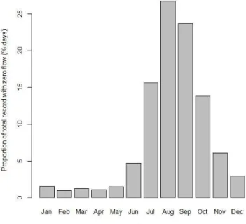
Fig. 3.Monthly variation in the occurrence of zero flow days. The days with zero flow in each month was computed from the flow records for all 123 intermittent gauges.
the procedure of Svetnik et al. (2004) to reduce the RF mod-els to the most parsimonious set of predictors. The procedure uses a cross-validation process that recursively removes the least-important predictors from the model and tests if the re-duced model has significantly lower prediction performance than the full model. We used the “1 standard error rule” (Breiman et al., 1984) to select the reduced model with the highest prediction performance that was not different, within the error generated from the cross-validation process, from the model with the best performance. The reduced models were considered to be the most parsimonious and we used these to interpret the relationships between predictors and the classifications.
We used a leave-one-out cross-validation procedure to es-timate the performance of the models and to optimize the probability threshold for the flow-regime model. In the cross-validation step, we fitted RF models to as many subsets of the data as there were gauging stations. For each subset, we withheld one gauging station in turn from the training data used to fit the RF models. We then used the RF model to independently predict the probability of the withheld station belonging to each of the classes represented by the classifi-cation. The cross-validated probabilities were then converted into predictions of class membership for each station based on a chosen probability threshold.
The performance of a classification model is sensitive to the probability threshold that is applied (Freeman and Moi-sen, 2008). We used receiver operating curves (ROCs) to pro-vide a method of evaluating the performance of the flow-regime model that was independent of the threshold. ROC
plots show the true positive rate (sensitivity) against the false positive rate (1-specificity) as the threshold varies from 0 to 1 (Hanley and McNeil, 1982). Good models have high true positive rates and relatively small false positive rates and, therefore, have curves that rise steeply at the origin, and level off near the maximum value of 1. The ROC plot for a poor model lies near the diagonal, where the true positive rate equals the false positive rate for all thresholds. The area under the ROC plot (AUC) is a measure of overall model performance that is independent of the threshold, with good models having an AUC near 1, while a poor models will have an AUC near 0.5 (Hanley and McNeil, 1982).
We used the cross-validation predictions for the flow-regime classification to derive ROC statistics to select the best threshold for assigning gauging stations to the peren-nial or intermittent class. There are several criteria that can be used to define the best threshold (Freeman and Moisen, 2008) including maximising the percent correctly classified (PCC) and maximising Cohen’s kappa (Cohen, 1960). Kappa measures the agreement between two classifications, each of which classifyNitems intoCmutually exclusive categories. We chose Kappa because it adjusts for chance agreement and is therefore a more robust measure than misclassification rate when observed occurrence is low (Freeman and Moisen, 2008). Kappa takes a value between 0 (no agreement) and 1 (complete agreement).
We also used the results of the cross-validation predictions and Kappa to characterise the performance of the intermit-tence classification model. We did not optimize the proba-bility threshold for the intermittence classification and sim-ply assigned stations to the intermittence sub-class with the highest probability.
3 Results
3.1 Zero flows and indices
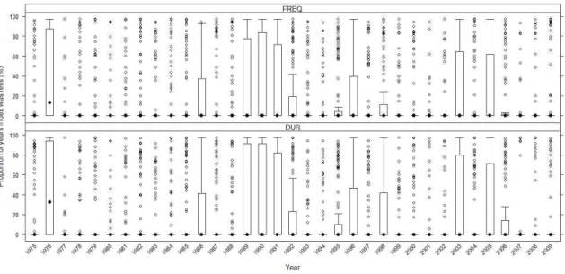
Fig. 4.Box plots of the annual variables (FREQ and DUR) for all years. The plots show data for only the gauging stations on intermittent segments. The variables have been standardized within stations by expressing them as the frequency that the index was less. Plotted values therefore indicate the severity of the zero-flow events in each year relative to the extremes observed at each station. The box contains the inter-quartile range, the dot shows the median value, whiskers indicate 1.5 times interquartile range and the circles indicate outliers.
The index mFREQ varied between 0 and 7.5 yr−1across
all 628 gauging stations. For stations on intermittent seg-ments, mFREQ ranged from 0.03 to 7.5 with a mean of 0.6 and a median of 0.3, indicating that most intermittent seg-ments had low zero-flow frequencies. For stations on inter-mittent segments, mDUR ranged from 1 to 128 days with a mean of 15 and a median of 7.3.
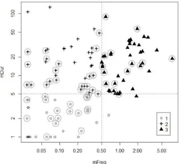
The two flow-intermittence indices mFREQ and mDUR were weakly, positively correlated (r=0.19, p= 0.03; Fig. 5). The intermittence subclasses 1, 2 and 3 comprised 41, 40 and 42 stations respectively. Three stations that fell just outside the ranges of mFREQ and mDUR that defined the subclasses and were assigned to the closest subclasses (lower right quadrant in Fig. 5). Gauging stations on inter-mittent river segments occurred across France; the highest densities were located near the southern and western coasts (Fig. 2). There was no clear geographic pattern evident in the spatial distribution of the three flow intermittence types (Fig. 2).
3.2 Spatial synchronization
The correlation coefficients (Mantelr)between dissimilar-ities corresponding to FREQ and DUR values for gauging stations on intermittent segments, and their spatial separa-tion were 0.1 and 0.14, respectively (p <0.0001; 10 000 per-mutations), indicating weak spatial synchronization. Mantel correlograms for both FREQ and DUR indicated that correla-tions were weak at all spatial scales (Fig. 6). The largest cor-relations were negative and occurred between stations with the largest separation (i.e., mean distances of 700 km).
3.3 Discrimination of intermittent and perennial gauging stations
The RF model that related the flow-regime classification of 628 gauging stations to environmental variables had a cross-validated AUC of 0.77. The performance of the RF model as measured by misclassification rate and Cohen’s kappa was sensitive to the probability value used as the threshold for assigning stations to either class (Fig. 7). The maximum per-cent correctly classified was 14.8 % and occurred at a prob-ability threshold of 0.49 (Fig. 7). The maximum Cohen’s kappa was 0.47 and occurred at a threshold of 0.35 (Fig. 7).
Fig. 5.Intermittence index values for gauging stations on intermit-tent segments. Three intermittence subclasses are indicated by dif-ferent symbols. Subclasses were defined using threshold values of mFREQ and mDUR (dashed lines). Sites that were misclassified by the RF model are indicated with gray circles.
When a probability threshold for the flow-regime model that maximized Cohen’s kappa (0.35) was used, 39 % of the digital river network segments were predicted to be intermittent (Fig. 10). When these predictions were aggre-gated into hydro-ecoregions, the proportion of intermittent segments in each region well predicted by the model. The regression of observed proportion of intermittent segments versus predicted proportion of intermittent segments had an
r2value of 0.73 (Fig. 10a).
The mapped predictions of the flow-regime model and the aggregation of these predictions into hydro-ecoregions highlighted a broad gradient in the probabilities of flow intermittence that corresponded to large-scale climate pat-terns (Figs. 9 and 10b). Regions with the highest propor-tion of intermittent segments tended to those with the low-est annual rainfall (Rain)<800 mm, the highest winter tem-perature (Tmin)>5◦C (Fig. 10b) and the highest summer
temperatures (Tmax)>20◦C. Regions with high
probabil-ities of flow intermittence were located along the Mediter-ranean and central Atlantic coasts, in the Midi-Pyr´en´ees re-gion (Fig. 9). In contrast, rere-gions with higher annual rainfall (Rain) >1100 mm, lower summer air temperature (Tmax)
<16◦C and lower winter air temperatures (Tmin)<1◦C had
high probabilities of perennial flow (Fig. 10b). There were additional, smaller regions in which river segments had high probabilities of flow intermittence. These regions were char-acterized by low values of hardness (Hard) and low slopes (Slope). There was also a general tendency for segments along large river main stems to have low probabilities of
be-Fig. 6.Mantel correlograms of FREQ and DUR for gauging stations on intermittent segments in nine distance classes. The plots indicate the Mantelrvalues for each distance class plotted against the mean separation of gauging stations in the class. Solid dots indicate sig-nificant Mantelrvalues (p <0.05) after Bonferroni correction.
Fig. 7.Receiver operating curves (ROC) plot (left) and threshold plot (right) for the flow-regime classification. The black circles on the threshold plot indicate the probabilities thresholds that maxi-mize the classification performance as measured by Cohen’s kappa and the percent correctly classified (PCC).
longing to the intermittent class (Fig. 9). Main stem segments had large values of catchment area (Area) and generally had low values of Shape, both of which were associated with low probabilities of flow intermittence (Figs. 8 and 9).
3.4 Discrimination of flow-intermittence patterns
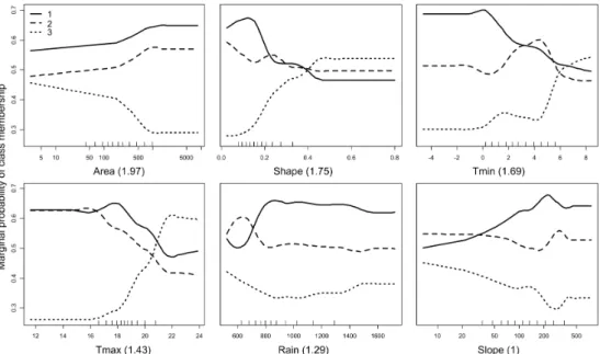
The RF model of the intermittence classification (classifica-tion of intermittent segments into three subclasses), had in-dependent misclassification rates of 51 %, 47 % and 31 % for classes 1, 2 and 3, respectively, and an overall misclassifica-tion rate of 46 % (Fig. 5). The value of kappa for the com-parison of predicted and actual membership of gauged river segments to the three intermittence types was 0.32.
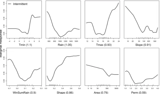
Fig. 8.Partial dependence of the probability of intermittence for each of significant environmental variables retained in the reduced model. The variables are shown in order of importance from the top-right to the bottom left. The plots show the marginal contribution to probability of flow intermittence (y-axis) as a function of the variables (i.e., the other contributing variables were held at their mean). The rug plots on the horizontal axes show deciles of the predictors. The value in brackets on the horizontal axis is the importance measure.
Fig. 9.Predictions of the probability of being intermittent made by the RF model of the flow-regime classification for the entire river network. Based on maximising Cohen’s kappa (Fig. 7), network segments whose probabilities are greater than 0.35 are intermittent and those less than 0.35 are perennial.
subPerm, subChalk, subLime, subAlluv) did not contribute significantly to model performance.
The partial plots indicated that the intermittence sub-classes were discriminated based on differences in catch-ment characteristics (Fig. 11). Subclass 1 (low-frequency, short-duration zero-flow periods) had highest probability of occurrence in large catchments with relatively high rainfall
Fig. 10. (A)Observed and predicted proportions of gauging stations on intermittent segments in hydro-ecoregions. The dashed line is the regression of observed versus predicted gauges on intermittent segments. The solid line indicates a perfect agreement between ob-served and predicted (i.e., slope = 1 and intercept = 0).(B)Scatter plot of the mean values of the most important predictor variables (Tmin and Rain) in each HER. The symbol sizes indicate the per-centage of gauges on intermittent segments each region.
Fig. 11.Partial dependence plots for the three flow intermittence subclasses for the six environmental variables retained in the reduced model, in order of importance from the top-right to the bottom left. The plots show the marginal contribution to probability of class membership (y-axis) as a function of the variable (i.e., the other contributing variables were held at their mean). The rug plots on the horizontal axes show deciles of the predictors. The value in brackets on the horizontal axis is the importance measure.
4 Discussion
In this study we used statistical models to identify rela-tionships between flow intermittence and catchment char-acteristics. To our knowledge, there have been no compa-rable studies that attempted to classify types of flow inter-mittence and predict its spatial distribution. Random forest models of the flow-regime and intermittence classifications had cross-validated kappa values that indicated only fair and poor performance respectively, based on the guidelines of Fleiss (1981). However, both classification models identified associations between intermittence and environmental vari-ables and provided some useful insights into the occurrence of flow intermittence.
Our models indicated significant associations and ex-pected relationships between intermittence and environmen-tal variables (Figs. 8 and 9). Regions with high probabili-ties of intermittent river segments are those with low annual rainfall, warm air temperatures, and steep, small, elongated catchments. The probability of intermittence had significant but more complex relationships with the environmental vari-ables SumWinRain and Perm. The similarity in importance values for the environmental variables retained in the RF model suggests that intermittence is caused by multiple phys-ical factors, each of which has a moderate influence.
The RF model of the intermittence classification identi-fied associations between environmental variables and dif-ferent combinations of zero-flow frequency and duration (Fig. 11). Based on its relationship with the environmental variables, intermittence Subclass 3 appears to represent
intermittence in France is only broadly associated with large-scale climate patterns (Figs. 9 and 10b). Flow intermittence is at least partly controlled by processes acting at smaller scales than climate, such as local groundwater-table fluctua-tions and seepage through permeable channels (Fleckenstein et al., 2006; Larned et al., 2010a, b). The proximate cause of flow intermittence in many river segments is water table fluc-tuation relative to river channel elevation; flow occurs when the water table intersects the channel, and ceases when the water table drops below the channel (Konrad, 2006; Larned et al., 2010a; von Schiller et al., 2011). In areas where chan-nels are permanently perched above the water table, intermit-tence is controlled by run-off from upstream and by transmis-sion losses (Morin et al., 2009; Sharma and Murthy, 1994). Interactions between these local processes and the climatic processes that generate runoff and rainfall recharge deter-mine where and when flow intermittence occurs. Two results lend support to the suggestion that intermittence, and in par-ticular, the timing of zero-flow periods, are only partly in-fluenced by large-scale climatic processes. First, the plots of annual zero-flow behavior (Fig. 4) and low values of Mantel statistics (Fig. 6) indicate that there was weak spatial syn-chronization in zero-flow frequency and duration. Although there was a general tendency for the frequency and duration of zero-flow periods to peak in the driest years of the time series (1976, 1989/1990, 2003), many sites did not follow this temporal pattern (Fig. 4). Second, the variables nDry-Days and dDry represent rainfall patterns that we expected to be more relevant to the duration and frequency of zero flows than mean annual rainfall, which was included in the RF models. However, these variables did not improve the classification models.
In contrast to the present study, a flow-regime classifica-tion of France reported by Snelder et al. (2009) distinguished river network segments on the basis of a variety of hydrolog-ical indices including the frequency of zero flow and others that described the frequency, timing and duration of high and low flows, and the frequency of changes in flow. A predictive model of this classification performed well and was based on similar statistical methods, and used the same river network and environmental variables used in the present study. We suggest that most of the flow-regime components described by the classification of Snelder et al. (2009) result predom-inantly from variation in large-scale processes such as rain-fall, evaporation, catchment storage and runoff. Variation in these processes over large spatial scales was reflected in rela-tively strong discrimination of flow-regime classes using the environmental variables.
The contrasting performance of the models in the present study with the model of the flow-regime classification of Snelder et al. (2009) indicates that different suites of environ-mental variables are needed to model intermittent flows and whole flow regimes (in which zero-flow frequency is only one of many components). Aquifer structure and riverbed permeability are probably among the factors that influence
the small-scale processes that determine intermittence and were represented in our models by variables such as catch-ment slope, shape and permeability. These variables had sim-ilar levels of importance in the RF models as the variables representing broad-scale climate, which supports our con-tention that processes at a range of scales are involved. How-ever, it is likely that, although these variables acted as sur-rogates for local processes, they were too broad scale and insufficiently representative of the actual causes of intermit-tency to achieve good predictive performance. The inclusion of predictor variables that described subcatchment (i.e., lo-cal) geology (Hard, Perm, Chalk, Lime, Alluv) was intended to provide better surrogates for small-scaled processes; how-ever, these did not improve model performance. It is likely that the 1 : 1 000 000 scale of the geological map used to de-fine the geological predictor variables was too coarse to dis-criminate geological or hydrogeological variation at segment scales. If flow intermittence is related to groundwater dynam-ics, spatial data corresponding to aquifer structure, riverbed permeability and other small-scale factors may improve our ability to model intermittent flows accurately, but these data are rarely available. Until that data scarcity is alleviated, pre-dictive models of regional or national patterns in flow inter-mittence will have limited accuracy.
Our predictions of the abundance and distribution of inter-mittent rivers in France will have several potential practical applications. First, the Water Framework Directive requires the ecological status of all surface and ground waters to be assessed (Chave, 2001), and this includes intermittent rivers. However, partly because they have been considered “atypi-cal” and rare in France, intermittent rivers have been often ignored by water managers. Our predictions may increase awareness of the prevalence of intermittent rivers among sci-entists and water managers by showing they are abundant and occur in most regions of France and are not restricted to the dry Mediterranean region.
Our flow-regime classification predictions indicate that the gauging station network under-represents intermittent river segments in France (i.e., 19.6 % of gauges were classified as intermittent whereas 39 % of segments in the river net-work are predicted to be intermittent). More accurate predic-tions of the abundance and distribution intermittent segments could be achieved by supplementing the gauging network. Alternative methods of monitoring flow intermittence, such as the use of electrical resistance arrays (Jaeger and Olden, 2012) or citizen-observation networks (Turner and Richter, 2011) could also increase the representation of intermittence in future studies at less effort than is required to operate per-manent gauging stations.
finer-resolution analysis would likely result in higher esti-mates of the proportion of intermittent segments. Other stud-ies have also concluded that lower order streams are more likely to be intermittent and represent a large proportion of river networks by length (Meyer et al., 2007).
Although predictions of intermittence were not accurate at the segment scale, when aggregated by HER they produced good estimates of the proportion of intermittent segments at regional scales (Fig. 10). Regional estimates of the propor-tion of intermittent segments provide important informapropor-tion for several management applications including environmen-tal flow setting (Hughes, 2005), estimating assimilative ca-pacity for contaminants (Tsagarakis et al., 2004) and design-ing bio-monitordesign-ing programs that are representative of the full range of river environments (Steward et al., 2011).
Finally, predictive models describing intermittence can be used to provide preliminary estimates of how climate change could change the frequency of intermittence (e.g., Benito et al., 2011). Our results suggest that the probability of intermit-tence in France would typically increase by approximately 2 % with each 1◦C rise in summer air temperature (Tmax)
and by 3 % for each 100 mm reduction in mean annual rain-fall (Rain) (Fig. 8).
Acknowledgements. Ton Snelder was supported by Marie Curie Incoming International Fellowship within the 6th European Community Framework Programme and by a joint Irstea-Onema research project on Low Flow Hydrology). We thank Andr´e Chan-desris for assistance with hydrological data and the French Water Agency Rhˆone-M´editerran´ee-Corse for financial support. We acknowledge the use of data supplied by the French database Banque Hydro and M´et´eo-France. Ton Snelder and Scott Larned were funded by the New Zealand Foundation for Research, Science and Technology, Environmental Flows Programme (C01X0308).
Edited by: D. Mazvimavi
References
Acu˜na, V., Mu˜noz, I., Giorgi, A., Omella, M., Sabater, F., and Sabater, S.: Drought and postdrought recovery cycles in an inter-mittent Mediterranean stream: structural and functional aspects, J. N. Am. Benthol. Soc., 24, 919–933, 2005.
Angel, R., Asaf, L., Ronen, Z., and Nejidat, A.: Nitrogen trans-formations and diversity of ammonia-oxidizing bacteria in a desert ephemeral stream receiving untreated wastewater, Micro-biol. Ecol., 59, 46–58, 2010.
Arscott, D. B., Larned, S., Scarsbrook, M. R., and Lambert, P.: Aquatic invertebrate community structure along an intermittence gradient: Selwyn River, New Zealand, J. Am. Water Resour. As., 29, 530–545, 2010.
Benichou, P. and Le Breton, O.: Prise en compte de la topographie pour la cartographie des champs pluviom´etriques statistiques (Use of topography on mapping of statistical rainfall fields), La M´et´eorologie, 7, 23–34, 1987.
Benito, G., Thorndycraft, V.R., Rico, M.T.: S´anchez-Moya, Y., Sope˜na, A., Botero, B. A., Machado, M. J., Davis, M., and P´erez-Gonz´alez, A.: Hydrological response of a dryland ephemeral river to southern African climatic variability during the last mil-lennium, Quaternary Res., 75, 471–482, 2011.
Bent, G. C. and Steeves, P. A.: A revised logistic regression equa-tion and an automated procedure for mapping the probability of a stream flowing perennially in Massachusetts, US Department of the Interior, US Geological Survey, 2006.
Booker, D. J. and Snelder, T. H.: Comparing methods for estimating flow duration curves at ungauged sites, J. Hydrol., 434–435, 78– 94, 2012
Breiman, L.: Random Forests, Mach. Learn., 45, 5–32, 2001. Breiman, L., Friedman, J. H., Olshen, R., and Stone, C. J.:
Classi-fication and Regression Trees, Wadsworth, Belmont, California, 1984.
BRGM: Carte g´eologique de France au 1/1.000.000`eme, 1996. Brooks, R. T. and Colburn, E. A.: Extent and channel morphology
of unmapped headwater stream segments of the Quabbin Wa-tershed, Massachusetts, J. Am. Water Resour. As., 47, 158–168, 2011.
Chave, P.: The EU Water Framework Directive: An Introduction, IWA Publishing, London, 2001.
Cohen, J.: A coefficient of agreement for nominal scales, Educ. Psy-chol. Meas., 20, 37–46, 1960.
Corti, R. and Datry, T.: Invertebrate and sestonic matter in an ad-vancing wetted front travelling down a dry riverbed (Albarine, France), Freshw. Sci. 31, 1187–1201, 2012.
Corti, R., Datry, T., Drummond, L., and Larned, S.: Leaf litter de-composition along the advancing-retreating front of a temporary river, Aquat. Sci., 73, 537–550, 2011.
Crocker, K. M., Young, A. R., Zaidman, M. D., and Rees, H. G.: Flow duration curve estimation in ephemeral catchments in Por-tugal, Hydrolog. Sci. J., 48, 427–439, 2003.
Cutler, D. R., Edwards, J. T. C., Beard, K. H., Cutler, A., Hess, K. T., Gibson, J., and Lawler, J. J.: Random forests for classification in ecology, Ecology, 88, 2783–2792, 2007.
Datry, T.: Benthic and hyporheic invertebrate assemblages along a flow intermittence gradient: effects of duration of dry events, Freshwater Biol., 57, 563–574, 2012.
Datry, T., Arscott, D., and Sabater, S.: Recent perspectives on tem-porary river ecology, Aquat. Sci., 73, 453–457, 2011
Datry, T., Corti, R., and Philippe, M.: Spatial and temporal aquatic– terrestrial transitions in the temporary Albarine River, France: responses of invertebrates to experimental rewetting, Freshwater Biol., 57, 716–727, 2012.
Davey, A. J. H. and Kelly, D. J.: Fish community responses to dry-ing disturbances in an intermittent stream: a landscape perspec-tive, Freshwater Biol., 52, 1719–1733, 2007.
Dieter, D., von Schiller, D., Garcia-Roger, E. M., S´anchez-Montoya, M. M., G´omez, R., Mora-G´omez, J., Sangiorgio, F., Gelbrecht, J., and Tockner, K.: Preconditioning effects of inter-mittent stream flow on leaf litter decomposition, Aquat. Sci., 73, 599–609, 2011.
Elmore, A. J. and Kaushal, S. S.: Disappearing headwaters: patterns of stream burial due to urbanization, Front. Ecol. Environ., 6, 308–312, 2008.
management, Ground Water, 44, 837–852, 2006.
Fleiss, J. L.: The measurement of interrater agreement, Statistical Methods for Rates and Proportions, 2, 212–236, 1981.
Freeman, E. A. and Moisen, G. G.: A comparison of the perfor-mance of threshold criteria for binary classification in terms of predicted prevalence and kappa, Ecol. Model., 217, 48–58, 2008. Friedman, J. H. and Meulman, J. J.: Multiple additive regression trees with application in epidemiology, Stat Med., 22, 1365– 1381, 2003.
Fritz, K. M., Johnson, B. R., and Walters, D. M.: Physical indicators of hydrologic permanence in forested headwater streams, J. Am. Water Resour. As., 27, 690–704, 2008.
G´omez, R., Hurtado, I., Su´arez, M., and Vidal-Abarca, M.: Ramblas in south-east Spain: threatened and valuable ecosystems, Aquat. Conserv., 15, 387–402, 2005.
Goslee, S. C. and Urban, D. L.: The ecodist package for dissimilarity-based analysis of ecological data, J. Stat. Softw., 22, 1–19, 2007.
Hanley, J. A. and McNeil, B. J.: The meaning and use of the area un-der a receiver operating characteristic (ROC) curve, Radiology, 143, 29–36, 1982.
Hansen, W. F.: Identifying stream types and management implica-tions, Forest Ecol. Manag., 143, 39–46, 2001.
Hastie, T., Tibshirani, R., and Friedman, J. H.: The Elements of Statistical Learning: Data Mining, Inference, and Prediction, Springer-Verlag, New York, 2001.
Heine, R. A., Lant, C. L., and Sengupta, R. R.: Development and comparison of approaches for automated mapping of stream channel networks, Ann. Assoc. Am. Geogr., 94, 477–490, 2004. Houston, J.: Variability of precipitation in the Atacama Desert: its causes and hydrological impact, Int. J. Climatol., 26, 2181–2198, 2006.
Hughes, D. A.: Hydrological issues associated with the determina-tion of environmental water requirements of ephemeral rivers, River Res. Appl., 21, 899–908, 2005.
Jacobson, P. and Jacobson, K.: Hydrologic controls of physical and ecological processes in Namib Desert ephemeral rivers: Impli-cations for conservation and management, J. Arid Environ., 93, 80–93, doi:10.1016/j.jaridenv.2012.01.010, 2013.
Jaeger, K. L. and Olden, J. D.: Electrical resistance sensor arrays as a means to quantify longitudinal connectivity of rivers, River Res. Appl., 28, 1843–1852, 2012.
Ji, X., Kang, E., Chen, R., Zhao, W., Zhang, Z., and Jin, B.: The impact of the development of water resources on environment in arid inland river basins of Hexi region, Northwestern China, Environ. Geol., 50, 793–801, 2006.
Katz, G. L., Denslow, M. W., and Stromberg, J. C.: The Goldilocks effect: intermittent streams sustain more plant species than those with perennial or ephemeral flow, Freshwater Biol., 57, 467–480, 2012.
Kennard, M. J., Pusey, B. J., Olden, J. D., Mackay, S. J., Stein, J. L., and Marsh, N.: Classification of natural flow regimes in Australia to support environmental flow management, Freshwa-ter Biol., 55, 171–193, 2010.
Kikawada, T., Minakawa, N., Watanabe, M., and Okuda, T.: Fac-tors inducing successful anhydrobiosis in the African chirono-mid Polypedilum vanderplanki: significance of the larval tubular nest, Integr. Comp. Biol., 45, 710–714, 2005.
Konrad, C.: Longitudinal hydraulic analysis of river-aquifer exchanges, Water Resour. Res., 42, 8425, doi:10.1029/2005WR004197, 2006.
Lake, P.: Ecological effects of perturbation by drought in flowing waters, Freshwater Biol., 48, 1161–1172, 2003.
Larned, S. T., Datry, T., Arscott, D. B., and Tockner, K.: Emerging concepts in temporary-river ecology, Freshwater Biol., 55, 717– 738, 2010a.
Larned, S. T., Arscott, D. B., Schmidt, J., and Diettrich, J. C.: A Framework for Analyzing Longitudinal and Temporal Variation in River Flow and Developing Flow-Ecology Relationships, J. Am. Water Resour. As., 46, 541–553, 2010b.
Larned, S. T., Schmidt, J., Datry, T., Konrad, C. P., Dumas, J. K., and Diettrich, J. C.: Longitudinal river ecohydrology: flow variation down the lengths of alluvial rivers, Ecohydrology, 4, 532–548, 2011.
Legendre, P. and Legendre, L.: Numerical ecology, Elsevier, Ams-terdam, the Netherlands, 1998.
Leibowitz, S. G., Wigington Jr., P. J., Rains, M. C., and Downing, D. M.: Non-navigable streams and adjacent wetlands: addressing science needs following the Supreme Court’s Rapanos decision, Front. Ecol. Environ., 6, 364–371, 2008.
Leopold, L. B.: A View of the River, Harvard Univ Press.California, 1994.
Mantel, N.: The detection of disease clustering and a generalized regression approach, Cancer Res., 27, 209–220, 1967.
Meirovich, L., Ben-Zvi, A., Shentsis, I., and Yanovich, E.: Fre-quency and magnitude of runoff events in the arid Negev of Is-rael, J. Hydrol., 207, 204–219, 1998.
Meyer, J. L., Strayer, D. L., Wallace, J. B., Eggert, S. L., Helfman, G. S., and Leonard, N. E.: The contribution of headwater streams to biodiversity in river networks, J. Am. Water Resour. As., 43, 86–103, 2007.
Morin, E., Grodek, T., Dahan, O., Benito, G., Kulls, C., Jacoby, Y., Langenhove, G. V., Seely, M., and Enzel, Y.: Flood routing and alluvial aquifer recharge along the ephemeral arid Kuiseb River, Namibia, J. Hydrol., 368, 262–275, 2009.
Nadeau, T. L. and Rains, M. C.: Hydrological connectivity between headwater streams and downstream waters: how science can in-form policy, J. Am. Water Resour. As., 43, 118–133, 2007. Olden, J. D., Kennard, M. J., and Pusey, B. J.: A framework
for hydrologic classification with a review of methodologies and applications in ecohydrology, Ecohydrology, 5, 503–518, doi:10.1002/eco.251, 2012.
Pella, H., Lejot, J., Lamouroux, N., and Snelder, T.: Le r´eseau hydrographique th´eorique (RHT) franc¸ais et ses attributs envi-ronnementaux (The theoretical hydrographical network (RHT) for France and its environmental attributes), G´eomorphologie, 3, 317–336, 2012.
Perry, S., Euverman, R., Wang, T., Loong, A., Chew, S., Ip, Y., and Gilmour, K.: Control of breathing in African lungfish (Pro-topterus dolloi): a comparison of aquatic and cocooned (terres-trialized) animals, Resp. Physiol. Neurobi., 160, 8–17, 2008. Quintana-Segui, P., Le Moigne, P., Durand, Y., Martin, E., Habets,
Sauquet, E. and Catalogne, C.: Comparison of catchment group-ing methods for flow duration curve estimation at ungauged sites in France, Hydrol. Earth Syst. Sci., 15, 2421–2435, doi:10.5194/hess-15-2421-2011, 2011.
Sayer, M. D. J.: Adaptations of amphibious fish for surviving life out of water, Fish. Fish., 6, 186–211, 2005.
Sharma, K. and Murthy, J.: Estimating transmission losses in an arid region – a realistic approach, J. Arid Environ., 27, 107–112, 1994.
Snelder, T. H., Pella, H., Wasson, J., and Lamouroux, N.: Defini-tion procedures have little effect on performance of environmen-tal classifications of streams and rivers, Environ. Manage., 42, 771–788, 2008.
Snelder, T. H., Lamouroux, N., Leathwick, J. R., Pella, H., Sauquet, E., and Shankar, U.: Predictive mapping of natural flow regimes of France, J. Hydrol., 373, 57–67, 2009.
Snelder, T., Ortiz, J. B., Booker, D., Lamouroux, N., Pella, H., and Shankar, U.: Can bottom-up procedures improve the perfor-mance of stream classifications?, Aquat. Sci., 74, 45–59, 2012. Steward, A. L., Marshall, J. C., Sheldon, F., Harch, B., Choy, S.,
Bunn, S. E., and Tockner, K.: Terrestrial invertebrates of dry river beds are not simply subsets of riparian assemblages, Aquat. Sci., 73, 551–566, 2011.
Svetnik, V., Liaw, A., Tong, C., and Wang, T.: Application of Breiman’s Random Forest to Modeling Structure-Activity Rela-tionships of Pharmaceutical Molecules, 5th International Work-shop on Multiple Classifier Systems, Springer, Cagliari, Italy, 334–343, 2004.
Tsagarakis, K. P., Dialynas, G., and Angelakis, A.: Water resources management in Crete (Greece) including water recycling and reuse and proposed quality criteria, Agr. Water Manage., 66, 35– 47, 2004.
Turner, D. S. and Richter, H. E.: Wet/dry mapping: using citizen sci-entists to monitor the extent of perennial surface flow in dryland regions, Environ. Manage., 47, 497–505, 2011.
von Schiller, D., Acu˜na, V., Graeber, D., Mart´ı, E., Ribot, M., Sabater, S., Timoner, X., and Tockner, K.: Contraction, fragmen-tation and expansion dynamics determine nutrient availability in a Mediterranean forest stream, Aquat. Sci., 73, 485–497, 2011. Wasson, J. G., Chandesris, A., Pella, H., and Blanc, L.: Typology
and reference conditions for surface water bodies in France: the hydro-ecoregion approach, TemaNord, 37–41, 2002.