Optical extinction by upper tropospheric/stratospheric aerosols and clouds: GOMOS observations for the period 2002–2008

(1)

ACPD

10, 11109–11138, 2010

GOMOS aerosol/cloud

extinction observations

F. Vanhellemont et al.

Title Page

Abstract Introduction

Conclusions References

Tables Figures

◭ ◮

Back Close

Full Screen / Esc

Printer-friendly Version

Interactive Discussion

Atmos. Chem. Phys. Discuss., 10, 11109–11138, 2010 www.atmos-chem-phys-discuss.net/10/11109/2010/ © Author(s) 2010. This work is distributed under the Creative Commons Attribution 3.0 License.

Atmospheric Chemistry and Physics Discussions

This discussion paper is/has been under review for the journal Atmospheric Chemistry and Physics (ACP). Please refer to the corresponding final paper in ACP if available.

Optical extinction by upper

tropospheric/stratospheric aerosols and

clouds: GOMOS observations for the

period 2002–2008

F. Vanhellemont1, D. Fussen1, N. Mateshvili1, C. T étard1, C. Bingen1, E. Dekemper1, N. Loodts1, E. Kyr öl ä2, V. Sofieva2, J. Tamminen2,

A. Hauchecorne3, J.-L. Bertaux3, F. Dalaudier3, L. Blanot3,4, O. Fanton d’Andon4, G. Barrot4, M. Guirlet4, T. Fehr5, and L. Saavedra5

1

Belgian Institute for Space Aeronomy, Brussels, Belgium 2

Finnish Meteorological Institute, Helsinki, Finland 3

Service d’A ´eronomie du CNRS, Verrieres-le-Buisson, France 4

ACRI-ST, Sophia-Antipolis, France 5

ESA-ESRIN, Frascati, Italy

Received: 26 January 2010 – Accepted: 20 April 2010 – Published: 26 April 2010 Correspondence to: F. Vanhellemont (filip.vanhellemont@aeronomie.be)

(2)

ACPD

10, 11109–11138, 2010

Title Page

Tables Figures

◭ ◮

Back Close

Full Screen / Esc

Interactive Discussion Abstract

Although the retrieval of aerosol extinction coefficients from satellite remote

measure-ments is notoriously difficult (in comparison with gaseous species) due to the lack

of typical spectral signatures, important information can be obtained. In this paper we present an overview of the current operational nighttime UV/Vis aerosol extinction

5

profile results for the GOMOS star occultation instrument, spanning the period from August 2002 to May 2008. Some problems still remain, such as the ones associated with incomplete scintillation correction and the aerosol spectral law implementation, but good quality extinction values can be expected at a wavelength of 500 nm. Typ-ical phenomena associated with atmospheric particulate matter in the Upper

Tropo-10

sphere/Lower Stratosphere (UTLS) are easily identified: Polar Stratospheric Clouds, tropical subvisual cirrus clouds, background stratospheric aerosols, and post-eruption volcanic aerosols (with their subsequent dispersion around the globe). In this overview paper we will give a summary of the current results.

1 Introduction

15

Upper tropospheric and stratospheric particles (whether liquid or solid) are intensively studied for a number of reasons that can be roughly summarized as follows: (1) they have an impact on the Earth radiative balance due to their optical properties, (2) they play a crucial role in heterogeneous chemistry, and (3) they provide information on the emission of precursor species from which they originate. Here, the word ’particles’

20

should be taken in its most general context: liquid or solid aerosols of submicron size, cloud droplets or crystals with sizes of tens or hundreds of microns, etc. From previous experiences with satellite occultation instruments, we know that a few particle types are commonly encountered in the measurements: stratospheric aerosols, tropical sub-visual cirrus clouds and Polar Stratospheric Clouds (PSCs).

25

(3)

ACPD

10, 11109–11138, 2010

Title Page

Tables Figures

◭ ◮

Back Close

Full Screen / Esc

Junge et al., 1961) consists of liquid droplets composed of a mixture of sulphuric acid and water. The layer manifests itself in a pronounced way after major volcanic

erup-tions that are powerful enough to inject teragrams of SO2into the stratosphere, such as

the ones of Mount Pinatubo (the Philippines, 1991) or El Chich ´on (Mexico, 1982); see Robock (2000). After an oxidation process, sulfate aerosols are formed that are

subse-5

quently transported globally, depending on the latitude of the eruption. Eventually they are removed from the stratosphere, although this process can take years. Neverthe-less, the last major eruption (Mount Pinatubo) dates already from 18 years ago, and the stratospheric aerosol layer returned to its “background” level around 1997. Since then, no significant trend is observed in data from SAGE II, balloon-borne instruments

10

and lidars (Deshler et al., 2003, 2006), even when compared with volcanically quiet years such as 1979. These findings suggest a more or less stable input of sulphuric species in the stratosphere that maintain the background layer. Crutzen (1976) sug-gested carbonyl sulfide (OCS) as the major precursor gas, although this hypothesis has been challenged (see e.g. Chin and Davis, 1995; Leung et al., 2002). Very recently,

15

increased anthropogenic SO2emission by coal burning in China has been proposed as

a possible origin for an upward trend in lidar measurements of stratospheric aerosols (Hofmann et al., 2009).

Polar Stratospheric Clouds have been investigated for over two decades now. The well-known classification scheme of PSCs was originally based on observations of

20

backscatter and depolarization ratios with lidar instruments (Poole and McCormick, 1988). Type Ia particles are believed to be relatively large crystalline particles

con-sisting of hydrates of HNO₃ such as Nitric Acid Trihydrate (NAT) or Dihydrate (NAD).

The smaller, liquid Type Ib particles consist of a supercooled ternary solution (STS) of HNO3, H2SO4 and H2O. The crystalline Type II particles are formed of pure water ice.

25

(4)

ACPD

10, 11109–11138, 2010

Title Page

Tables Figures

◭ ◮

Back Close

Full Screen / Esc

below about 195 K, while the Type II ice crystals form at the ice frost point, about 188 to 190 K in the lower stratosphere. These cold temperatures are provided in the polar regions during local winter.

The so-called subvisual cirrus clouds are a fairly recent discovery for the obvious reason that they are optically thin and thus invisible from the ground (hence the name):

5

an upper limit for the optical thickness of 0.03 at 694 nm is sometimes mentioned in the literature. Long optical pathlengths ensure that satellite occultation instruments such as SAGE II have detected them frequently (Wang et al., 1996). They are mainly found in the tropics and midlatitudes, around the tropopause altitude region (16–17 km). Much is still to be learned about the formation of these clouds, but Jensen et al. (1996)

10

proposed at least two mechanisms: (1) they originate from horizontal anvil-shaped out-flows of large convective cumulonimbus clouds, and (2) from nucleation inside a humid layer that experiences slow uplift through the extremely cold region of the tropopause. Subvisual cirrus form cloud layers with a very large horizontal extent (hundreds of kilo-meters) but are at the same time very thin (smaller than 1 km). In recent years they

15

received a lot of attention due to their possible role in the radiative balance of the atmosphere, their impact on ozone concentrations through heterogeneous chemistry (Solomon et al., 1997), and their role in the dehydration of air that enters the tropical lower stratosphere (Jensen et al., 1996).

The Global Ozone Monitoring by Occultation of Stars (GOMOS) instrument was

pri-20

marily intended to deliver accurate altitude profiles of trace gas concentrations. These retrievals can be performed since each gas is detected by its specific spectral signa-ture in the measured light intensity. Atmospheric particle populations pose a more challenging problem since the spectral shape is unknown, with the direct consequence that it is a priori impossible to find out which kind of particles are in the line of sight of

25

(5)

ACPD

10, 11109–11138, 2010

Title Page

Tables Figures

◭ ◮

Back Close

Full Screen / Esc

spectral dependence). However, the distinction will be made in this paper with the use of additional information, such as time of appearance/disappearance, geolocation and altitude.

First results on GOMOS aerosol/cloud extinction profiles representing the year 2003 were previously published (Vanhellemont et al., 2005). This paper presents results for

5

the period 2002–2008.

2 GOMOS: instrument and obtained data set

The GOMOS instrument has been adequately described elsewhere (Kyr ¨ol ¨a et al., 2004; Bertaux et al., 1991, 2000, 2010), so we only give a brief summary here. GO-MOS, onboard ENVISAT, was launched in a sunsynchroneous orbit on 1 March 2002.

10

GOMOS routine operations started in August 2002, and since then the instrument has been recording data almost continuously until present. GOMOS observes occultations of stars (chosen from a predefined catalogue) behind the earth limb, and records the received light intensity in the UV/Vis/NIR spectral range: 248–690 nm (spectrometers A1 and A2), 755–774 nm (spectrometer B1) and 926–954 nm (spectrometer B2). From

15

measured signals, transmittances are calculated that in turn are used to derive alti-tude concentration profiles for O₃, NO₂, NO₃, H₂O and O₂, and temperature profiles.

Furthermore, aerosol/cloud extinction profiles at different wavelengths are obtained.

It is important to know that the uncertainty on the obtained profiles is largely deter-mined by the magnitude and temperature of the observed star. But even bright stars

20

(such as Sirius) are weak light sources in comparison with the Sun; profiles obtained from stellar occultations have therefore larger uncertainties than the ones from solar occultations. This disadvantage is however largely compensated for by the fact that stars are abundant in the sky: about 30 to 40 occultations have been typically ob-served per orbit, although this number decreased to 20 or 30 occultations per orbit

25

(6)

ACPD

10, 11109–11138, 2010

Title Page

Tables Figures

◭ ◮

Back Close

Full Screen / Esc

The occultation statistics for the period August 2002–May 2008 (a total of about 600 000 events, the entire data set that was available to us at the time of writing) are represented by histograms in Fig. 1. Of course, the lower number of occultations for the years 2002 and 2008 are caused by an incomplete sampling of these years, while the smaller number in 2005 resulted from the instrument failure mentioned earlier.

Longi-5

tudinal sampling is clearly very homogeneous. Most occultations occur at midlatitudes, although plenty of polar measurements are available. Most stars have moderate to weak brightness, and are rather cold. Also, about half of the occultations occur in the Sun-illuminated atmosphere (“bright limb”, Solar Zenith Angle SZA<100), the other half

in “dark limb” (SZA≥100). More details about the solar illumination condition and its

10

consequences are given below.

3 Retrieval method

3.1 Spectral behaviour

As already said above, the particle optical extinction spectrum is a priori unknown. Therefore, the actual optical spectrum is treated as a product of the retrieval algorithm.

15

It is far from clear how such a particle optical spectrum should be parameterized, but we can be guided by the fact that usual atmospheric particle size distributions are broad, covering a few orders of magnitude, and the resulting optical spectra are thus smooth. Hence they are often described with analytic, smooth functions, such as polynomi-als. For data version 6.0, the GOMOS Science team chose to implement a quadratic

20

polynomial as a function of wavelength for the simple reason that it is versatile: large (constant spectrum), medium-sized (peak at mid-visible wavelengths) or small

parti-cle spectra (β∼λ−4) can within good approximation be captured by such polynomials.

Retrieval algorithms for other satellite occultation instruments are often also equipped with this feature. Furthermore, Vanhellemont et al. (2006) showed with simulated data

25

(7)

ACPD

10, 11109–11138, 2010

Title Page

Tables Figures

◭ ◮

Back Close

Full Screen / Esc

obtain good aerosol retrievals without introducing too many degrees of freedom in the retrieval problem.

3.2 Spectral/spatial inversion

The GOMOS retrieval algorithm has been described in detail in another paper of this special issue (Kyr ¨ol ¨a et al., 2010). Here it suffices to say that the retrieval consists of

5

two parts: (1) the spectral inversion, where measured transmittance spectra at each tangent altitude separately are inverted to slant path integrated column densities (for gases) and optical thickness (for particles), and (2) the spatial or vertical inversion, where the retrievals of the first step are separately inverted to local concentration pro-files (gases) and optical extinction propro-files (particles). This second step is performed

10

in combination with a Tikhonov altitude smoothing (Twomey, 1985; Rodgers, 2000) in order to get partially rid of the perturbations caused by residual scintillation in mea-surements taken during very inclined occultations (Sofieva et al., 2009). The amount of smoothing is determined by a predetermined target resolution for the profile. For particles, a profile resolution of 4 km was chosen since unsmoothed profiles showed

15

strong oscillations; aerosol extinction spectra have the tendency to swallow a large por-tion of the residual scintillapor-tion perturbapor-tions. Nevertheless, fine-scale structures (e.g. thin clouds) are smeared out due to this feature.

It is in the spectral inversion model that the slant path particle optical thickness is implemented as a quadratic polynomial:

20

τ(λ)=σref(r0+r1∆λ+r2∆λ2)

with ∆λ=λ−λref and λref=500 nm a reference wavelength. For scaling purposes, a

“cross section” σref=6·10− 10

cm2 was used. Notice that only the first parameter r0

has a direct physical meaning:σrefr0equals the particle slant path optical thickness at 500 nm. During the spatial inversion, this parameter receives Tikhonov-style altitude

25

(8)

ACPD

10, 11109–11138, 2010

Title Page

Tables Figures

◭ ◮

Back Close

Full Screen / Esc

turned out to be a poor methodology: while the obtained extinction profiles at 500 nm look quite good, the spectra at other wavelengths are often very noisy.

Finally, it should be mentioned that during the spectral inversion, the optical extinc-tion spectra from the neutral air (Rayleigh scattering) are removed instead of retrieved from the measurements, using external ECMWF (European Centre for Medium-range

5

Weather Forecasts) air density data, to avoid interferences with the residual scintilla-tion and the spectrally similar aerosol contribuscintilla-tion. Also, only spectrometer A measure-ments are currently used for the aerosol retrieval.

3.3 The homogeneous layer assumption

Occultation measurements have a limited information content. Hence the assumption

10

of homogeneous atmospheric layers that is so often found in retrieval codes: the num-ber of unknowns is drastically reduced, leading to a more stable inversion. For more or less uniformly mixed gases and particles (such as stratospheric aerosols), the as-sumption should hold quite well. However, when local phenomena (such as clouds)

are observed, the assumption is wrong: the phenomenon a_ffects the light ray only

lo-15

cally. This should be taken into account whenever we analyse retrievals of PSCs and

volcanic plumes, for example: the obtained extinction coefficients should be seen as

slant path equivalent values.

3.4 Bright limb versus dark limb retrievals

When the optical light path traverses the Sun-illuminated atmosphere, parts of the

at-20

mosphere located in the field-of-view scatter additional light into the instrument, which means that the simple optical transmission model for the retrieval is not correct any-more. This was anticipated: the additionnal upper and lower CCD bands in GOMOS were implemented to correct for this background illumination (Bertaux et al., 2010; Kyr ¨ol ¨a et al., 2010). However, post-launch processing showed that the correction is not

25

(9)

ACPD

10, 11109–11138, 2010

Title Page

Tables Figures

◭ ◮

Back Close

Full Screen / Esc

smooth optical extinction spectrum strongly resembles the limb signal. The aerosol ex-tinction retrievals typically show unrealistic features at very high stratospheric altitudes. At present, the best we can do is exclude the bright limb profiles from data analysis. Investigations showed that occultation events with a solar zenith angle of 100◦or larger deliver unperturbed, dark limb aerosol retrievals.

5

3.5 Retrieval results

In summary, the GOMOS particle extinction profiles have acceptable quality around 500 nm, but are oversmoothed. At other wavelenghts, the profile quality is poor, and we therefore exclude them from further study. Furthermore, it is best to exclude the aerosol profiles in bright limb (SZA<100): from the entire data set of 600 000

occul-10

tations, about 301 000 remain to be exploited. Among these, some are still perturbed by residual scintillation. These perturbations are visible in individual aerosol extinction profiles. When averaging large numbers of profiles (see e.g. the zonal plots below), the perturbations disappear, confirming that they are random in nature, with zero mean.

Like all profiles derived from occultation measurements, GOMOS aerosol extinction

15

profiles are increasingly more uncertain when we descend to lower altitudes, because

the transmitted light intensity becomes weaker. In principle, a cut-offaltitude can be

defined, below which no aerosol information is present anymore. This altitude depends on the wavelength considered, and the magnitude and temperature of the star, and therefore changes from one occultation to the next. At 500 nm, an average limit of

20

10 km can be considered as the value below which the profiles are not trustworthy anymore.

On Fig. 2, we present individual GOMOS extinction retrievals at 500 nm for a number of particle types. It is impossible to distinguish these types using only one wavelength; the presented profiles were selected after analysis of the entire GOMOS data set and

25

knowledge about geolocation and time of occurence of these particle phenomena (see further on in this paper).

(10)

ACPD

10, 11109–11138, 2010

Title Page

Tables Figures

◭ ◮

Back Close

Full Screen / Esc

are known to be horizontally extended cloud layers that are quite thin, having a thick-ness smaller than 1 km (Jensen et al., 1996); the example on the figure clearly shows that the layer has been spread out by the smoothing constraint.

4 Comparisons with other instruments

A detailed validation study for the GOMOS aerosol extinction profiles has not been

per-5

formed yet. Nevertheless, Vanhellemont et al. (2008) already performed comparisons with the results derived from the imagers of the Atmospheric Chemistry Experiment ACE (Bernath et al., 2005). Here, we present first comparisons with aerosol extinc-tion profiles from the Stratospheric Aerosol and Gas Experiment II (SAGE II; see Chu et al., 1989), its follow-up SAGE III (Thomason and Taha, 2003) and the Polar Ozone

10

and Aerosol Measurement POAM III (Lucke et al., 1999). As already stated, only dark limb measurements were considered. Furthermore we avoided PSCs by excluding oc-cultations inside the polar vortex: apart from the wrong assumption of homogeneous layers, two different instruments with two different viewing geometries will deliver two

different profiles for the same cloud. A coincidence window of 500 km and 1/2 day was

15

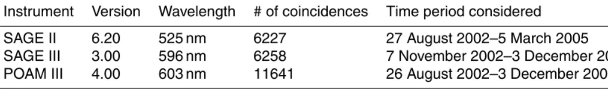
used, allowing us to find a fairly large comparison data set, summarized in Table 1. Notice that we used a spectral channel of each instrument that is close to the GO-MOS reference wavelength of 500 nm. Furthermore, GOGO-MOS data were interpolated to these wavelengths using the retrieved quadratic polynomial.

For the i-th coincidence, the difference between GOMOS (GOM) and the other

in-20

strument (SAT), relative to the mean of the two, was evaluated as follows:

∆i=100×2

(pGOM,i−pSAT,i)

|pGOM,i+pSAT,i|

As statistical estimators for the entire data set, we prefered to use the median (50th percentile) since it is more robust with respect to outliers than the numerical mean. The variance of the data set was calculated with the 16th and 84th percentile. The obtained

(11)

ACPD

10, 11109–11138, 2010

Title Page

Tables Figures

◭ ◮

Back Close

Full Screen / Esc

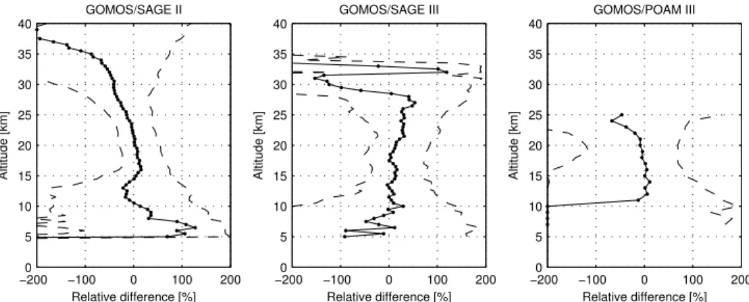
statistical estimates are shown in Fig. 3. As can be seen, the comparisons are quite

good at upper tropospheric/lower stratospheric altitudes. Differences with SAGE II are

within 20% from 10 to 25 km, a conclusion that can also be drawn for the SAGE III

comparisons. The median differences with POAM III are even smaller, within 10% from

11 to 22 km. Notice however that the variance is much larger than for the SAGE II/III

5

comparisons.

5 Results

5.1 Yearly zonal statistics

A coarse idea about the presence of aerosols and clouds in the upper tropo-sphere/lower stratosphere can be gained by considering zonal yearly statistics.

Rang-10

ing from 90◦S to 90◦N, 72 latitude bins with a width of 2.5 degrees were defined.

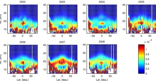
Aerosol extinction profiles were linearly interpolated on a common altitude grid ranging from 1 to 50 km with a spacing of 1 km. Yearly statistics were subsequently calculated on all data within one bin. Once again: we used percentiles as statistical estimators since extinction values are not necessarily normally distributed and because the

me-15

dian (50th percentile) is rather insensitive to outliers. We should also mention that yearly zonal statistics are seasonally biased when we use only dark limb measure-ments, since Arctic/Antarctic summer is not sampled. The median particle extinction at 500 nm is shown in Fig. 4 for every GOMOS mission year. A few phenomena are readily observed: (1) the umbrella-shaped stratospheric aerosol layer that is highest at

20

the equator, lowest at the poles, (2) higher extinction values in the Antarctic (and to a lesser extent Arctic) stratosphere that are caused by PSCs, and (3) higher extinction values in a localized tropical zone at an altitude of about 16–17 km due to subvisual cirrus clouds. The picture is almost systematic for every year, but there are some

signif-icant differences however. First notice that Antarctic PSCs are less pronounced for the

25

(12)

ACPD

10, 11109–11138, 2010

Title Page

Tables Figures

◭ ◮

Back Close

Full Screen / Esc

years: the data set starts end of August 2002 and ends in May 2008. More important, stratospheric aerosol extinction levels are much higher in 2007 and remain elevated even in 2008, suggesting the formation of new aerosols following stratospheric injec-tion of SO2 by a volcanic eruption. This is the case; the Soufri `ere Hills eruption (see below) in May 2006 is most likely the source. Furthermore, 2005 also seems to exhibit

5

elevated aerosol levels, although the picture is noisier due to the incomplete sampling of the year (instrument failure).

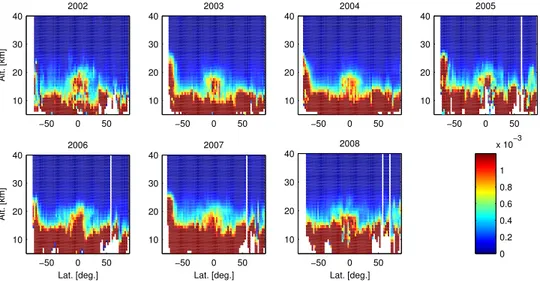
Equally interesting is the yearly zonal variability of the 500 nm aerosol extinction

values, calculated as half the difference between the 84th and 16th percentile. The

variability is of course determined by the S/N-ratio of the measurements and (more

10

importantly) by natural aerosol/cloud variability, caused by the appearing, disappear-ing and atmospheric transport of particles. This is clearly visible on Fig. 5. Typical

“on/off-events” such as clouds (tropical cirrus, PSCs) exhibit large variability, while

slowly changing features (such as the stratospheric aerosol layer) vary little within one year. Notice once again that the Antarctic PSC variability during 2002 and 2008 is weak

15

since these years have not been completely sampled. At lower, tropospheric altitudes, we see large variability due to a combination of larger profile uncertainty (measured signals are weaker) and tropospheric clouds.

5.2 Volcanic stratospheric aerosols

The observed elevated extinction levels in 2005 and 2007 require a more detailed

in-20

vestigation. On Fig. 6, we present aerosol extinction values at an altitude of 20 km (which lies above the subvisual cirrus altitudes) for the period 2004–2006, in a

trop-ical latitude band from 6◦N to 26◦N. Three distinct periods can be seen. First, we

observe low background aerosol levels until the end of 2004. Second, from early 2005 to the beginning of June 2006, large data gaps are present due to instrument failure.

25

(13)

ACPD

10, 11109–11138, 2010

Title Page

Tables Figures

◭ ◮

Back Close

Full Screen / Esc

levels. The same conclusions are drawn when inspecting the evolution in latitude and time on Fig. 7. It is clear that at least two volcanic events in the tropics should be considered.

The elevated values in 2005 are most likely caused by stratospheric sulfate aerosols,

formed out of the SO₂cloud injected in the stratosphere by the eruptions of the Manam

5

volcano (Papua New Guinea, 4.080◦S, 145.037◦E) on 27 and 28 January (Kamei et al.,

2006). Manam is one of the most active volcanoes in the region; the above mentioned eruptions followed ongoing volcanic activity that started already in October 2004. An image taken by the infrared Aqua/MODIS (Moderate Resolution Imaging Spectrora-diometer) indicates that the ash clouds of the first eruption on 27 January reached to

10

over 20 km altitude, well into the stratosphere. The ash clouds of the second eruption on 28 January ascended to 18 km altitude (Smithsonian Institution, 2005). Several days later, stratospheric aerosol layers were detected twice between about 18 to 20 km alti-tude (layer thickness ranging from 0.2 to 1.4 km) by a shipboard lidar using a Nd:YAG laser operated at 1064 nm and 532 nm (Kamei et al., 2006). The layers were detected

15

in the Western Pacific around 0–2◦N, 156◦E (3–4 February 2005) and 7–9◦N, 156◦E

(9–10 February). Inspecting Fig. 7, we see that the amount of injected sulfur was large enough to leave a significant aerosol trace in the GOMOS data during the largest part of 2005.

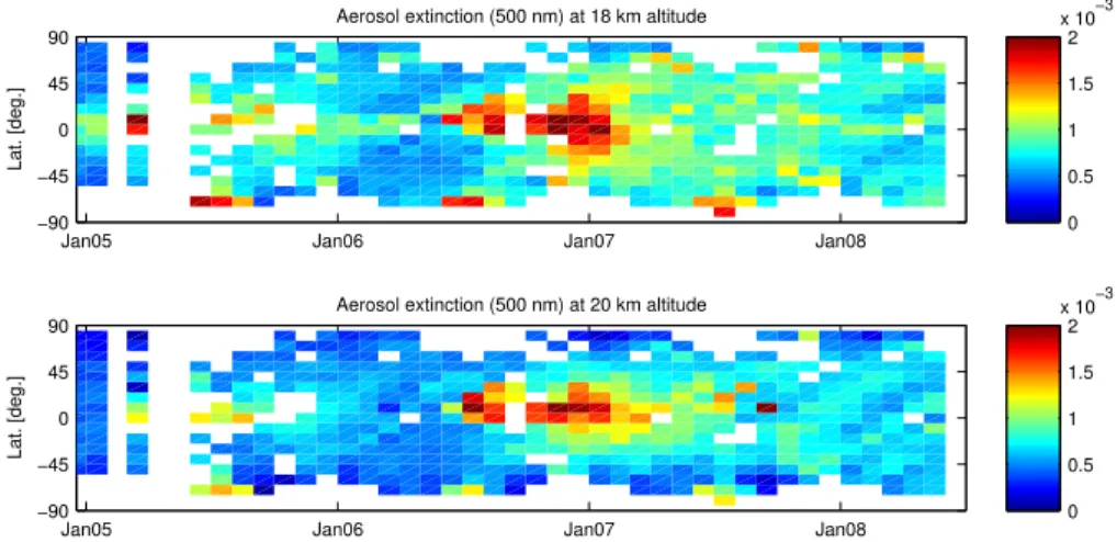
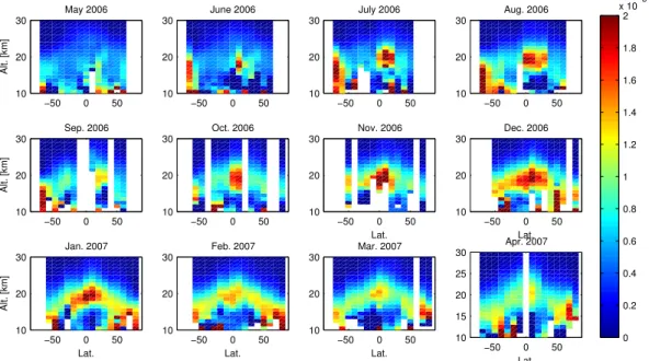
The source for the elevated aerosol levels in the second half of 2006 and 2007

20

has been identified as the eruption of the Soufri `ere Hills volcano (16.72◦N, 62.18◦W, Montserrat, West Indies), on 20 May 2006. Immediately following the collapse of the eastern volcano flank, an eruption column of ash and gases rose to at least 17 km. Prata et al. (2007) used a combination of satellite instruments (Aqua/AIRS, MSG/SEVIRI, MLS, OMI and CALIPSO/CALIOP) to reconstruct the event and its

im-25

mediate aftermath. They found that an estimated 0.1 Tg(S) was injected in the

strato-sphere in the form of SO₂, after which the gas cloud traveled westward at an altitude

of about 20 km. Carn et al. (2007) on the other hand used OMI data to obtain an

(14)

ACPD

10, 11109–11138, 2010

Title Page

Tables Figures

◭ ◮

Back Close

Full Screen / Esc

measurements of the associated stratospheric aerosol layer as early as 7 June 2006, at an altitude of 20 km. The layer remained visible in the CALIOP data until 6 July. However, as Thomason et al. (2007) remarked, in general the stratospheric aerosol layer remains quite invisible in CALIOP backscatter measurements, while occulation instruments such as SAGE II have no problem with the detection. No doubt this is

5

caused by the preferential forward scattering of light by small particles, in combination with longer optical path lengths. The fact that GOMOS identifies stratospheric sulfate aerosols well after the eruption date is illustrated in Fig. 8, which shows the appearing and poleward transport of the sulfuric acid particles.

Figures 7 and 8 also indicate that it took roughly one year for the Soufri `ere Hills

10

aerosol cloud to cover the entire globe. Elevated extinction levels remained present until at least the end of 2007. In the months following the Soufri `ere Hills eruption, a few other eruptions possibly impacted the stratospheric aerosol layer. Hofmann et al.

(2009) briefly mentioned the 14 July 2006 Tungurahua eruption (Ecuador, 1.467◦S,

78.442◦W), less than a month after the Soufri `ere Hills eruption. And Thomason et al.

15

(2007) showed CALIOP observations of the volcanic plume resulting from the 7

Octo-ber 2006 Tavurvur eruption (Rabaul, Papua New Guinea, 4.271◦S, 152.203◦E). Both

are equatorial volcanoes that possible injected sulfur into the stratosphere, hereby en-hancing the already existing Soufri `ere Hills perturbation. From GOMOS data it is at present unclear wether or not the existing volcanic aerosol layer was replenished with

20

new sulfate aerosols originating from these eruptions.

5.3 Polar Stratospheric Clouds

GOMOS observes PSCs quite well. Strongly enhanced optical extinction is measured every year in the Antarctic PSC season (roughly from the end of May to October), with values typically 3 or 4 times larger than in normal background conditions. These kind

25

(15)

ACPD

10, 11109–11138, 2010

Title Page

Tables Figures

◭ ◮

Back Close

Full Screen / Esc

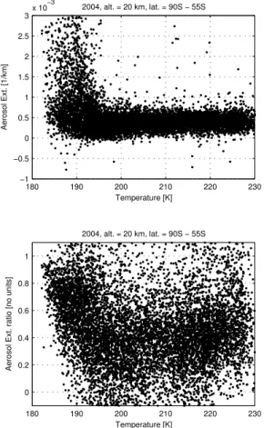
aerosol extinction measurements at 500 nm taken in 2004 at an altitude of 20 km for the

latitude band from 90◦S to 55◦S. This data set represents a mixture of measurements

inside and outside the Antarctic vortex (PSCs and stratospheric aerosols), but plotted

against temperature the differentiation is very clear: clouds are formed below about

195 K, the known formation temperature of NAT and STS PSCs. It is however less

5

clear from the data whether or not Type II PSCs form at even lower temperatures. Ideally, differentiation of different types of PSC with UV/Vis/NIR data should be done by inspecting particle size distributions, or the shape of the associated optical spectrum. Methods have already been devised in the past for the SAGE and POAM instruments to make a distinction between Type Ia and Ib particles, based on the assumption that the

10

latter are smaller than the former, with a di_fferent extinction spectrum as a consequence (Strawa et al., 2002; Poole et al., 2003). The second panel of Fig. 9 shows the ratio of 600 nm to 400 nm GOMOS optical extinction. Theoretically, very small particles (β(λ)∼λ−4) should lead to a value of 0.2, while large particles (β(λ)₌constant) should have a value of 1. The data are extremely noisy due to the already mentioned problem

15

with the aerosol spectral law implementation. Nevertheless, the data cloud is more or less situated between the theoretical limits, and larger particles are observed below

195 K, as expected. The data show also that it is currently impossible to differentiate

between different PSC types.

6 Conclusions

20

The current GOMOS operational aerosol/cloud product consists of optical extinction profiles at 500 nm and additional spectral coefficients to evaluate the extinction at other wavelengths as well. The quality of the product is not optimal yet, due to a problematic spectral law implementation, combined with an altitude smoothing that is too strong. Furthermore, profiles derived from bright limb measurements are currently not usable.

25

(16)

ACPD

10, 11109–11138, 2010

Title Page

Tables Figures

◭ ◮

Back Close

Full Screen / Esc

fine structure (thin cirrus clouds, cloud inhomogeneities etc.) has been smoothed. A comparison with SAGE II, SAGE III and POAM III showed good agreement within 20% in the upper troposphere/lower stratosphere, from 10 km to about 25 km.

All the atmospheric particle types that are expected to be observed by a satellite oc-cultation instrument have been detected by GOMOS: the background stratospheric

5

sulfate aerosol layer (or Junge layer) with its typical umbrella-shaped form, sulfate aerosols from volcanic origin, tropical subvisual cirrus clouds just below the tropopause at an altitude of about 16–17 km, and PSCs in the polar regions. The cloud-type events (PSCs and cirrus) have a strong yearly variability, while the Junge layer remains re-markably constant within one year.

10

The last major volcanic SO₂injection into the stratosphere dates already from almost

18 years ago (Mount Pinatubo, 1991), with the consequence that current aerosol

lev-els are extremely low. So low that the effect of “moderate” volcanic eruptions becomes

visible in the GOMOS aerosol record. One might wonder if the so-called background is not only maintained by the typically mentioned sources (OCS, recently even

an-15

thropogenic sulfate from coal burning in China), but as well by these moderate volcanic eruptions, that are much weaker than the catastrophic events (Mt. Pinatubo, Mt. St. He-lens, El Chich ´on), but much more frequent. In the GOMOS data, the aerosol enhance-ments resulting from the eruptions of Manam (Papua New Guinea) and Soufri `ere Hills (Montserrat, West Indies) have been identified. In the latter case, GOMOS was clearly

20

able to track the global dispersion of the aerosols. In the aftermath of the eruption, two other possible intrusions should in principle be visible: Tungurahua (Ecuador) and Tavurvur (Papua New Guinea). We hope to identify them in future aerosol profile im-provements.

The dynamics of PSCs have been studied previously with GOMOS data

(Vanhelle-25

(17)

ACPD

10, 11109–11138, 2010

Title Page

Tables Figures

◭ ◮

Back Close

Full Screen / Esc

As of February 2009, our team has been involved in a new project (AERGOM, an ESA financed project) to develop an improved algorithm that should deliver significantly better aerosol extinction profiles (at all GOMOS wavelengths) in the close future. A cloud-Type Identification method will also be devised. This will enable us to derive particle size distributions, and to study the microphysics of the observed particle

phe-5

nomena.

Acknowledgements. This work came into existence with the financial aid of the Belgian Federal Science Policy Office (BELSPO) and the European Space Agency (ESA) through the AERGOM project (Contract No. 22022/08/I-OL). ENVISAT is an ESA mission andGOMOS is an EFI (ESA Funded Instrument).

10

References

Bernath, P. F., McElroy, C. T., Abrams, M. C., Boone, C. D., Butler, M., Camy-Peyret, C., Carleer, M., Clerbaux, C., Coheur, P.-F., Colin, R., DeCola, P., DeMazi `ere, M., Drummond, J. R., Dufour, D., Evans, W. F. J., Fast, H., Fussen, D., Gilbert, K., Jennings, D. E., Llewellyn, E. J., Lowe, R. P., Mahieu, E., McConell, J. C., McHugh, M., McLeod, S. D., Michaud, R.,

15

Midwinter, C., Nassar, R., Nichitiu, F., Nowlan, C., Rinsland, C. P., Rochon, Y. J., Rowlands, N., Semeniuk, K., Simon, P., Skelton, R., Sloan, J. J., Soucy, M. A., Strong, K., Tremblay, P., Turnbull, D., Walker, K. A., Walkty, I., Wardle, D. A., Wehrle, V., Zander, R., and Zou, J.: Atmospheric Chemistry Experiment (ACE): Mission overview, Geophys. Res. Lett., 32, L15S01, doi:10.1029/2005GL022386, 2005. 11118

20

Bertaux, J., Kyr ¨ol ¨a, E., and Wehr, T.: Stellar occultation technique for atmospheric ozone mon-itoring: GOMOS on Envisat, Earth observation quarterly, 17–20, 2000. 11113

Bertaux, J. L., Megie, G., Widemann, T., Chassefi ère, E., Pellinen, R., Kyr öl ä, E., Korpela, S., and Simon, P.: Monitoring of ozone trend by stellar occultations: The GOMOS instrument, Adv. Space Res., 11, 3237–3242, 1991. 11113

25

(18)

ACPD

10, 11109–11138, 2010

Title Page

Tables Figures

◭ ◮

Back Close

Full Screen / Esc

10, 9917–10076, 2010,

http://www.atmos-chem-phys-discuss.net/10/9917/2010/. 11113, 11116

Carn, S. A., Krotkov, N. A., Yang, K., Hoff, R. M., Prata, A. J., Krueger, A. J., Loughlin, S. C., and Levelt, P. F.: Extended observations of volcanic SO₂and sulfate aerosol in the stratosphere, Atmos. Chem. Phys. Discuss., 7, 2857–2871, 2007,

5

http://www.atmos-chem-phys-discuss.net/7/2857/2007/. 11121

Chin, M. and Davis, D. D.: A reanalysis of carbonyl sulfide as a source of stratospheric back-ground sulfur aerosol, J. Geophys. Res., 100, 8993–9005, 1995. 11111

Chu, W., McCormick, M., Lenoble, J., Brogniez, C., and Pruvost, P.: SAGE II inversion algo-rithm, J. Geophys. Res., 94, 8339–8351, 1989. 11118

10

Crutzen, P.: The possible importance of OCS for the sulfate layer of the stratosphere, Geophys. Res. Lett., 3, 73–76, 1976. 11111

Deshler, T., Hervig, M. E., Hofmann, D. J., Rosen, J. M., and Liley, J. B.: Thirty years of in situ stratospheric aerosol size distribution measurements from Laramie, Wyoming (41N), using balloon-borne instruments, J. Geophys. Res., 108(D5), 4167, doi:10.1029/2002JD002514,

15

2003. 11111

Deshler, T., Anderson-Sprecher, R., J ¨ager, H., Barnes, J., Hofmann, D. J., Clemesha, B., Si-monich, D., Osborn, M., Grainger, R. G., and Godin-Beeckmann, S.: Trends in the non-volcanic component of stratospheric aerosol over the period 1971–2004, J. Geophys. Res., 111, D01201, doi:10.1029/2005JD006089, 2006. 11111

20

Hofmann, D., Barnes, J., O’Neill, M., Trudeau, M., and Neely, R.: Increase in background stratospheric aerosol observed with lidar at Mauna Loa Observatory and Boulder, Colorado, Geophys. Res. Lett., 36, L15808, doi:10.1029/2009GL039008, 2009. 11111, 11122

Jensen, E. J., Toon, O. B., Selkirk, H. B., Spinhirne, J. D., and Schoeberl, M. R.: On the for-mation and persistence of subvisible cirrus clouds near the tropical tropopause, J. Geophys.

25

Res., 101, 21361–21375, 1996. 11112, 11118

Junge, C., Chagnon, C., and Manson, J.: Stratospheric aerosols, J. Meteorol., 18, 80–108, 1961. 11111

Kamei, A., Sugimoto, N., Matsui, I., Shimizu, A., and Shibata, T.: Volcanic aerosol layer ob-served by shipboard lidar over the tropical western Pacific, Scientific Online Letters on the

30

Atmosphere, 2, 001–004, doi:10.2151/sola.2006-001, 2006. 11121

(19)

ACPD

10, 11109–11138, 2010

Title Page

Tables Figures

◭ ◮

Back Close

Full Screen / Esc

B., Guirlet, M., Etanchaud, F., Snoeij, P., Koopman, R., Saavedra, L., Fraisse, R., Fussen, D., and Vanhellemont, F.: GOMOS on Envisat – an overview, Adv. Space Res., 33, 1020–1028, 2004. 11113

Kyr ¨ol ¨a, E., Tamminen, J., Sofieva, V., Bertaux, J. L., Hauchecorne, A., Dalaudier, F., Fussen, D., Vanhellemont, F., Fanton d’Andon, O., Barrot, G., Guirlet, M., Mangin, A., Blanot, L.,

5

Fehr, T., Saavedra de Miguel, L., and Fraisse, R.: Retrieval of atmospheric parameters from GOMOS data, Atmos. Chem. Phys. Discuss., 10, 10145–10217, 2010,

http://www.atmos-chem-phys-discuss.net/10/10145/2010/. 11115, 11116

Leung, F.-Y. T., Colussi, A. J., Hoffmann, M. R., and Toon, G. C.: Isotopic fractionation of car-bonyl sulfide in the atmosphere: Implications for the source of background stratospheric

sul-10

fate aerosol, Geophys. Res. Lett., 29(10), 1474, doi:10.1029/2001GL013955, 2002. 11111 Lucke, R. L., Korwan, D. R., Bevilacqua, R., Hornstein, J. S., Shettle, E. P., Chen, D. T., Daehler,

M., Lumpe, J. D., Fromm, M. D., Debrestian, D., Ne_ff, B., Squire, M., K ¨onig-Langlo, G., and Davies, J.: The Polar Ozone and Aerosol Measurement (POAM) III instrument and early validation results, J. Geophys. Res., 104, 18785–18799, 1999. 11118

15

Poole, L. R. and McCormick, M. P.: Airborne lidar observations of Arctic polar stratospheric clouds: Indications of two distinct growth stages, Geophys. Res. Lett., 15, 21–23, 1988. 11111

Poole, L. R., Trepte, C. R., Harvey, V. L., Toon, G. C., and Van Valkenburg, R. L.: SAGE III observations of Arctic polar stratospheric clouds – December 2002, Geophys. Res. Lett.,

20

30(23), 2216, doi:10.1029/2003GL018496, 2003. 11123

Prata, A. J., Carn, S. A., Stohl, A., and Kerkmann, J.: Long range transport and fate of a stratospheric volcanic cloud from Soufri `ere Hills volcano, Montserrat, Atmos. Chem. Phys., 7, 5093–5103, 2007,

http://www.atmos-chem-phys.net/7/5093/2007/. 11121

25

Robock, A.: Volcanic eruptions and climate, Rev. Geophys., 38, 191–219, 2000. 11111 Rodgers, C.: Inverse Methods for Atmospheric Sounding – Theory and Practice, World

Scien-tific, first edn., 2000. 11115

Smithsonian Institution: Bulletin of the Global Volcanism Network, 30(2): February 2005, Manam, online available at: http://www.volcano.si.edu/reports/bulletin, (last access: April

30

2010) 2005. 11121

(20)

ACPD

10, 11109–11138, 2010

Title Page

Tables Figures

◭ ◮

Back Close

Full Screen / Esc

GOMOS, Atmos. Chem. Phys., 9, 9197–9207, 2009, http://www.atmos-chem-phys.net/9/9197/2009/. 11115

Solomon, S., Borrmann, S., Garcia, R. R., Portmann, R., Thomason, L., Poole, L. R., Winker, D., and McCormick, M. P.: Heterogeneous chlorine chemistry in the tropopause region, J. Geophys. Res., 102, 21411–21429, 1997. 11112

5

Strawa, A. W., Drdla, K., Fromm, M., Pueschel, R. F., Hoppel, K. W., Browell, E. V., Hamill, P., and Dempsey, D. P.: Discriminating Types Ia and Ib polar stratospheric clouds in POAM satellite data, J. Geophys. Res., 107(D20), 8291, doi:10.1029/2001JD000458, 2002. 11123 Thomason, L. W., Pitts, M. C., and Winker, D. M.: CALIPSO observations of stratospheric

aerosols: a preliminary assessment, Atmos. Chem. Phys., 7, 5283–5290, 2007,

10

Thomason, L. W. and Taha, G.: SAGE III aerosol extinction measurements: Initial results, Geophys. Res. Lett., 30(12), 1631, doi:10.1029/2003GL017317, 2003. 11118

Twomey, S.: Introduction to the Mathematics of Inversion in Remote Sensing and Indirect Mea-surements, Elsevier Scientific Publishing Company, New York, USA, 1985. 11115

15

Vanhellemont, F., Fussen, D., Bingen, C., Kyr öl ä, E., Tamminen, J., Sofieva, V., Hassinen, S., Verronen, P., Sepp äl ä, A., Bertaux, J. L., Hauchecorne, A., Dalaudier, F., Fanton d’Andon, O., Barrot, G., Mangin, A., Theodore, B., Guirlet, M., Renard, J. B., Fraisse, R., Snoeij, P., Koopman, R., and Saavedra, L.: A 2003 stratospheric aerosol extinction and PSC climatol-ogy from GOMOS measurements on Envisat, Atmos. Chem. Phys., 5, 2413–2417, 2005,

20

http://www.atmos-chem-phys.net/5/2413/2005/. 11113, 11124

Vanhellemont, F., Fussen, D., Dodion, J., Bingen, C., and Mateshvili, N.: Choosing a suitable analytical model for aerosol extinction spectra in the retrieval of UV/visible satellite occultation measurements, J. Geophys. Res., 111, D23203, doi:10.1029/2005JD006941, 2006. 11114 Vanhellemont, F., Tetard, C., Bourassa, A., Fromm, M., Dodion, J., Fussen, D., Brogniez, C.,

25

Degenstein, D., Gilbert, K. L., Turnbull, D. N., Bernath, P., Boone, C., and Walker, K. A.: Aerosol extinction profiles at 525 nm and 1020 nm derived from ACE imager data: com-parisons with GOMOS, SAGE II, SAGE III, POAM III, and OSIRIS, Atmos. Chem. Phys., 8, 2027–2037, 2008,

30

(21)

ACPD

10, 11109–11138, 2010

Title Page

Tables Figures

◭ ◮

Back Close

Full Screen / Esc

Table 1. GOMOS aerosol extinction retrievals: comparison data set; coincidence window: (500 km, 1/2 day).

(22)

ACPD

10, 11109–11138, 2010

Title Page

Tables Figures

◭ ◮

Back Close

Full Screen / Esc

2002 2004 2006 2008 0

0.5 1 1.5 2

x 105

Year

# occultations

−180 −90 0 90 180 0

0.5 1 1.5 2

x 104

Longitude [degrees]

# occultations

−90 −45 0 45 90 0

1 2 3

x 104

Latitude [degrees]

# occultations

−2 0 2 4

0 5 10 15x 10

4

Star magnitude

# occultations

0 1 2 3 4

x 104 0

0.5 1 1.5

2x 10

5

Star temperature [K]

# occultations

50 100 150 0

1 2 3 4x 10

4

Solar zenith angle [degrees]

# occultations

(23)

ACPD

10, 11109–11138, 2010

Title Page

Tables Figures

◭ ◮

Back Close

Full Screen / Esc

0 2 4

x 10−3 10

20 30 40 50

Extinction [km−1]

Altitude [km]

Polar stratospheric cloud

0 2 4

x 10−3 10

20 30 40 50

Extinction [km−1]

Altitude [km]

Tropical subvisual cirrus

0 2 4

x 10−3 10

20 30 40 50

Extinction [km−1]

Altitude [km]

Background aerosol

0 2 4

x 10−3 10

20 30 40 50

Extinction [km−1]

Altitude [km]

Volcanic aerosol

(24)

ACPD

10, 11109–11138, 2010

Title Page

Tables Figures

◭ ◮

Back Close

Full Screen / Esc

−2000 −100 0 100 200 5

10 15 20 25 30 35 40

GOMOS/SAGE II

Relative difference [%]

Altitude [km]

−2000 −100 0 100 200 5

10 15 20 25 30 35 40

GOMOS/SAGE III

Altitude [km]

−2000 −100 0 100 200 5

10 15 20 25 30 35 40

GOMOS/POAM III

Altitude [km]

Fig. 3. Comparison of GOMOS aerosol extinction profiles with other satellite measurements: SAGE II at 525 nm (left panel), SAGE III at 596 nm (middle panel) and POAM III at 603 nm (right panel). Shown are the statistics for the relative differences, calculated as 100×2(p_GOMOS−

p_SAT)/|p_GOMOS+p_SAT|. The median of the set of relative differences is shown with full lines and

(25)

ACPD

10, 11109–11138, 2010

Title Page

Tables Figures

◭ ◮

Back Close

Full Screen / Esc

−50 0 50 10

20 30 40

2002

Alt. [km]

−50 0 50 10

20 30 40

2003

−50 0 50 10

20 30 40

2004

−50 0 50 10

20 30 40

2005

−50 0 50 10

20 30 40

2006

Lat. [deg.]

Alt. [km]

−50 0 50 10

20 30 40

2007

Lat. [deg.]

−50 0 50 10

20 30 40

2008

Lat. [deg.]

0 0.2 0.4 0.6 0.8 1 x 10−3

(26)

ACPD

10, 11109–11138, 2010

Title Page

Tables Figures

◭ ◮

Back Close

Full Screen / Esc

−50 0 50 10

20 30 40

2002

Alt. [km]

−50 0 50 10

20 30 40

2003

−50 0 50 10

20 30 40

2004

−50 0 50 10

20 30 40

2005

−50 0 50 10

20 30 40

2006

Alt. [km]

Lat. [deg.]

−50 0 50 10

20 30 40

2007

Lat. [deg.]

−50 0 50 10

20 30 40

2008

Lat. [deg.]

0 0.2 0.4 0.6 0.8 1 x 10−3

(27)

ACPD

10, 11109–11138, 2010

Title Page

Tables Figures

◭ ◮

Back Close

Full Screen / Esc

Feb04 Jun04 Sep04 Dec04 Mar05 Jul05 Oct05 Jan06 May06 Aug06 Nov06 −1

−0.5 0 0.5 1 1.5 2 2.5

3x 10

−3

Aerosol. Ext. [1/km]

Date

2004 to 2006 − Aerosol ext. 500 nm, alt = 20 km, lat = 6N − 26N

(28)

ACPD

10, 11109–11138, 2010

Title Page

Tables Figures

◭ ◮

Back Close

Full Screen / Esc

Jan05 Jan06 Jan07 Jan08 −90

−45 0 45 90

Lat. [deg.]

Aerosol extinction (500 nm) at 18 km altitude

0 0.5 1 1.5 2 x 10−3

Jan05 Jan06 Jan07 Jan08 −90

−45 0 45 90

Lat. [deg.]

Aerosol extinction (500 nm) at 20 km altitude

0 0.5 1 1.5 2 x 10−3

(29)

ACPD

10, 11109–11138, 2010

Title Page Abstract Introduction Conclusions References Tables Figures ◭ ◮ ◭ ◮ Back Close

Full Screen / Esc

−50 0 50 10

20 30

Alt. [km]

May 2006

−50 0 50 10

20 30

June 2006

−50 0 50 10

20 30

July 2006

−50 0 50 10

20 30

Aug. 2006

−50 0 50 10

20 30

Alt. [km]

Sep. 2006

−50 0 50 10

20 30

Oct. 2006

−50 0 50 10

20 30

Lat. Nov. 2006

−50 0 50 10

20 30

Lat. Dec. 2006

−50 0 50 10 20 30 Lat. Alt. [km] Jan. 2007

−50 0 50 10

20 30

Lat. Feb. 2007

−50 0 50 10

20 30

Lat. Mar. 2007

−50 0 50 10 15 20 25 30 Lat. Apr. 2007 0 0.2 0.4 0.6 0.8 1 1.2 1.4 1.6 1.8 2 x 10−3

(30)

ACPD

10, 11109–11138, 2010

Title Page

Tables Figures

◭ ◮

Back Close

Full Screen / Esc

180 190 200 210 220 230 −1

−0.5 0 0.5 1 1.5 2 2.5 3

x 10−3

Temperature [K]

Aerosol Ext. [1/km]

2004, alt. = 20 km, lat. = 90S − 55S

180 190 200 210 220 230 0

0.2 0.4 0.6 0.8 1

Temperature [K]

Aerosol Ext. ratio [no units]

2004, alt. = 20 km, lat. = 90S − 55S