www.atmos-meas-tech.net/9/4687/2016/ doi:10.5194/amt-9-4687-2016
© Author(s) 2016. CC Attribution 3.0 License.
AerGOM, an improved algorithm for stratospheric aerosol
extinction retrieval from GOMOS observations –
Part 1: Algorithm description
Filip Vanhellemont1, Nina Mateshvili1, Laurent Blanot3, Charles Étienne Robert1, Christine Bingen1,
Viktoria Sofieva2, Francis Dalaudier4, Cédric Tétard1, Didier Fussen1, Emmanuel Dekemper1, Erkki Kyrölä2,
Marko Laine2, Johanna Tamminen2, and Claus Zehner5
1Belgisch Instituut voor Ruimte-Aëronomie/Institut d’Aéronomie Spatiale de Belgique, Brussels, Belgium 2Finnish Meteorological Institute, Helsinki, Finland
3ACRI-ST, Sophia Antipolis, France
4Laboratoire Atmosphères, Milieux, Observations Spatiales, Guyancourt, France 5ESA-ESRIN, Frascati, Italy
Correspondence to:Filip Vanhellemont ([email protected])
Received: 28 January 2016 – Published in Atmos. Meas. Tech. Discuss.: 5 February 2016 Revised: 24 August 2016 – Accepted: 25 August 2016 – Published: 21 September 2016
Abstract.The GOMOS instrument on Envisat has success-fully demonstrated that a UV–Vis–NIR spaceborne stellar occultation instrument is capable of delivering quality data on the gaseous and particulate composition of Earth’s at-mosphere. Still, some problems related to data inversion re-mained to be examined. In the past, it was found that the aerosol extinction profile retrievals in the upper troposphere and stratosphere are of good quality at a reference wave-length of 500 nm but suffer from anomalous, retrieval-related perturbations at other wavelengths. Identification of algo-rithmic problems and subsequent improvement was there-fore necessary. This work has been carried out; the resulting AerGOM Level 2 retrieval algorithm together with the first data version AerGOMv1.0 forms the subject of this paper. The AerGOM algorithm differs from the standard GOMOS IPF processor in a number of important ways: more accurate physical laws have been implemented, all retrieval-related covariances are taken into account, and the aerosol extinc-tion spectral model is strongly improved. Retrieval examples demonstrate that the previously observed profile perturba-tions have disappeared, and the obtained extinction spectra look in general more consistent. We present a detailed vali-dation study in a companion paper; here, to give a first idea of the data quality, a worst-case comparison at 386 nm shows SAGE II–AerGOM correlation coefficients that are up to 1
order of magnitude larger than the ones obtained with the GOMOS IPFv6.01 data set.
1 Introduction
The sounding of planetary atmospheres by observation of astronomical objects (Sun, Moon, planets, stars) in occul-tation is a well-established technique. Spaceborne Earth observation instruments such as SAGE II (Chu et al., 1989), SAGE III (Thomason et al., 2010), ORA (Fussen et al., 2001), POAM III (Lucke et al., 1999), ACE–Maestro (Bernath et al., 2005; McElroy et al., 2007) and GOMOS (Bertaux et al., 2010) have clearly demonstrated the possi-bility to obtain altitude-resolved profiles for a number of at-mospheric gaseous species and particles (aerosols, clouds), through the combination of occultation transmittance mea-surements with a dedicated data inversion algorithm. For ob-vious reasons, most instruments use the Sun as light source, although the geographical coverage and temporal sampling (at most twice per orbit) is limited. Stellar occultation largely resolves these problems (due to the abundance of stars), how-ever at the cost of a reduced measurementS/Nratio.
of papers have been published in the scientific literature that describe the instrument, data processing, and the ob-tained scientific results for the different atmospheric species; a good overview article has been published by Bertaux et al. (2010). Notwithstanding this success, several problems re-garding the instrument and the data processing posed diffi-culties. Most noteworthy, the imperfect correction of stellar scintillation due to isotropic turbulence (Sofieva et al., 2009) remains a problem, though the associated residual scintilla-tions have been adequately characterized in a statistical anal-ysis (Sofieva et al., 2010). The random nature of these per-turbations causes them to disappear after averaging of binned constituent profiles. More important within the context of this paper, aerosol–cloud extinction profile retrievals are of good quality at 500 nm (Vanhellemont et al., 2008, 2010) but suffer from unphysical perturbations at other wavelengths within the GOMOS spectral range. This problem was already identified earlier (Vanhellemont et al., 2005) but has been left unexamined until now.
From a retrieval point of view, the importance of good aerosol–cloud extinction retrievals lies in the fact that they are intrinsically linked with the retrieval quality of the other species; specifically, upper troposphere–lower strato-sphere (UTLS) ozone values are significantly biased due to erroneous aerosol retrievals (Tamminen et al., 2010). Scien-tifically, good aerosol–cloud extinction observations in the UTLS and stratosphere are of main importance for atmo-spheric research, in two ways: (1) the Earth radiative budget depends on the optical properties of high-altitude clouds and volcanic sulfate aerosols, and (2) heterogeneous polar ozone chemistry is driven by the presence of polar stratospheric clouds (PSCs), stratospheric aerosols and high-altitude cir-rus clouds. A good overview of the scientific significance of aerosols–clouds can be found in the SPARC report (SPARC, 2006).
Improvement of a long-term aerosol–cloud data record such as the one provided by GOMOS is therefore important. The European Space Agency (ESA) has acknowledged this by funding the AerGOM project (Aerosol profile retrieval prototype for GOMOS). Within this project framework, data inversion problems have been studied, solutions have been found, and a new Level 2 algorithm has been developed.
In this article, we summarize the essentials of the GO-MOS instrument and its operational data processing algo-rithm (currently IPF v6.01). Subsequently, we present and justify the specific features that have been changed in the AerGOM code. Finally, the AerGOM aerosol–cloud extinc-tion results are discussed in a qualitative way; a detailed data validation is presented in a companion paper (Robert et al., 2016).
2 GOMOS and its operational data processor 2.1 Instrument and measurement principle
The GOMOS instrument and measurement principles are described elsewhere (see e.g. Kyrölä et al., 2004; Bertaux et al., 2000, 2010). GOMOS (Global Ozone Monitoring by Occultation of Stars), a UV–Vis–NIR grating spectrometer on board ESA’s Envisat satellite, was launched into a sun-synchronous orbit on 1 March 2002. Routine operations started in August 2002, and continued almost uninterrupt-edly until the end of the mission on 8 April 2012, when con-tact with the satellite was lost. Using the method of stellar occultation, GOMOS was able to monitor ozone (its main target gas), a number of other trace gases and aerosols, at al-titudes that fall within the range from the upper troposphere to the top of the atmosphere. In total, almost a million occul-tations have been registered by GOMOS during its 10-year mission, roughly half of them in dark limb conditions (local nighttime).
Spectrally, GOMOS is a medium-resolution instrument, designed with ozone monitoring in mind. To obtain ozone profiles from the UTLS (using the Chappuis band) to the upper mesosphere (using the Hartley band), two spectrome-ters SPA1 and SPA2 were included, covering the UV–visible wavelength range (248–690 nm); apart from ozone, this spec-tral range also allows for the measurement of optical ab-sorption by NO2, NO3, and the extinction (scattering) by
aerosols and air. Other trace gases such as OClO and Na are also detectable with specific statistical methods. Further-more, a spectrometer B1 (SPB1) was added (spectral range 755–774 nm), with the purpose of measuring absorption in the O2A band. Finally, a spectrometer B2 (SPB2) in the
near-IR wavelength range (926–954 nm) allows the measurement of water vapour. The GOMOS spectrometer characteristics are summarized in Table 1.
It was realized in an early stage of the GOMOS devel-opment that stellar scintillation would perturb the measure-ments considerably. In order to remove this perturbation, GOMOS was equipped with two fast photometers, sampling the blue (473–527 nm) and the red (646–698 nm) spectral do-main at a frequency of 1 kHz. Apart from the scintillation correction (which was only partially achieved; see further in the text), the time delay between the two photometer signals due to chromatic refraction has been used to obtain altitude profiles of refractive index and temperature.
deter-Table 1.GOMOS spectral bands. The number of pixels for each band and the optically active species are also indicated.
Spectral band Wavelength range No. pixels Resolution Major absorbing–scattering species
SPA1 & SPA2 248–690 nm 1416 0.8 nm neutral density, O3, NO2, NO3, aerosols–clouds SPB1 775–774 nm 420 0.13 nm neutral density, O2, aerosols–clouds
SPB2 926–954 nm 500 0.13 nm neutral density, H2O, aerosols–clouds
mined by its obliquity: an occultation within the orbital plane is vertical and therefore short (about 40 s), while observa-tions at an angle with the orbital plane are slant, with a long duration (up to several minutes). It is clear that, for a fixed acquisition time per spectrum, better altitudinal sampling is obtained for long occultation durations.
Finally, it should be mentioned that the measurementS/N
ratio is largely determined by the apparent brightness and the temperature of the star; the catalogue used by GOMOS contains objects with visual magnitudes smaller than 4 and temperatures ranging from 3000–30 000 K (i.e. most stellar spectral types). The combined effects of varying obliquities and star characteristics lead to a GOMOS data set that has in a sense an inhomogeneous nature; during data analysis, the variation in altitudinal sampling andS/N ratio has to be
taken into account.
2.2 IPFv6.01 operational data processing 2.2.1 Assumptions and initial processing
It is not the purpose of this paper to describe in detail the GOMOS operational data processing chain. It is nevertheless necessary to give a general overview, in order to highlight the differences with the AerGOM processor further in the text. Detailed descriptions can be found in Kyrölä et al. (2010, 2012). Before the actual data inversion from measurements to geophysical products is performed, downlinked data are formatted, ancillary data are added, the necessary calibration steps are taken and erroneous measurements (e.g. resulting from cosmic ray impacts) are flagged. The contribution of star scintillation to transmittance is estimated from the data of the two photometers and is removed from the spectrometer data. As was mentioned in the introduction, this correction is incomplete since residual scintillation due to isotropic turbu-lence is not accounted for.
The subsequent Level 2 processing steps are based on a number of assumptions and corrections. (1) The Earth is globally described by a WGS84 reference ellipsoid (NIMA, 1984). Locally, the Earth is approximated by a tangent sphere with a radius equal to the one given by the WGS84 model. (2) Chromatic refraction leads to different tangent points for different wavelengths. A data reinterpolation is performed such that one entire transmittance spectrum is associated with the same tangent point. (3) A correction for refractive dilu-tion is applied. The phenomenon is caused by the altitude gradient of the air refractive index and consists of the
spread-ing of light rays (divergence) and an associated decrease in light flux. (4) The finite spectral response of the instrument is taken into account by applying a convolution of theoret-ical or lab-measured cross sections with the instrument re-sponse function. (5) Slant path aerosol optical depth (SAOD) is modelled as a quadratic polynomial of wavelength:
τaer(λ)=τaer(λref)h1+c1(λ−λref)+c2(λ−λref)2i, (1)
withλrefa reference wavelength of 500 nm, andτaer(λref),c1
andc2parameters to be fitted. A quadratic polynomial can fit
a wide range of spectral shapes, representing small particles (τ∼λ−4), submicron-sized particles (spectra peaking in the
visible wavelength range) to large particles (τ =constant). (6) The variance of the residual scintillation component in the signals due to isotropic turbulence is taken into account by adding an extra term to the measurement covariance ma-trix. This so-called full covariance matrix (FCM) method has been described by Sofieva et al. (2010).
The Level 2 inversion is of course based on the Beer– Lambert law for optical extinction. Furthermore, the entire inversion is divided in two separate subproblems: (1) a spec-tral inversion from individual transmittance spectra to slant path integrated gas column densities (SGDs; unit: cm−2) and
aerosol optical depths (SAODs; unitless), and (2) a spatial inversion from these slant path integrated quantities to local gas density and aerosol extinction altitude profiles. The main advantage of this processing chain lies in its numerical effi-ciency: a large number of measurements (transmittance spec-tra) are reduced to a small number of slant path integrated quantities in an early stage of the processing.
2.2.2 Spectral inversion
The SPB1 and SPB2 spectrometers were primarily meant for oxygen and water vapour measurements. To separate the pro-cessing of these two species, it was decided to obtain all other species exclusively from SPA1 and SPA2 data. As an ini-tial step, to avoid correlations between the spectrally simi-lar aerosol and air scattering contributions, the latter is eval-uated from ECMWF (European Centre for Medium-Range Weather Forecasts) temperature and pressure forecasts and is removed. The other contributions (O3, NO2 and NO3
SGDs; aerosol SAODs) are obtained by fitting the remain-ing transmittanceTremwith the Beer–Lambert law (using a
SGD retrievals suffered badly from the residual scintillation in the measurements; it was decided to fit both species by making use of their differential spectral features, in a DOAS-like manner (differential optical absorption spectroscopy).
At the final iteration of each individual spectral fit, the ob-tained covariance matrix is evaluated from the forward model Jacobian. It should be emphasized that the fit is performed for every tangent altitude separately; the retrieval covariances between species at different altitudes are therefore equal to zero.
2.2.3 Spatial inversion
The obtained SGDs and SAODs are equal to the integral of the local gas densities and aerosol extinction coefficients along the optical path. An appropriate discretization of this integral leads to a linear forward model. For example, the model equations for the column vectors representing alti-tude profiles for the ozone SGDNO3and the 500 nm aerosol SAODτaer,500equal
NO3=GnO3 τaer,500=Gβaer,500,
with thenO3 andβaer,500vectors representing altitude pro-files for the ozone density (molecules cm−3) and 500 nm
aerosol extinction (cm−1). The square triangular matrix G
contains optical path length contributions: the matrix element Gij equals the path length for a ray with tangent point radius ritthrough the atmospheric layer centred atrjt.
The spatial inversion then consists of finding a solution for the unknown local altitude profiles (nO3,βaer,500etc.), using a linear least-squares method, subject to a Tikhonov smooth-ing constraint. The associated merit function to be minimized reads (for ozone, as an example)
M=[NO3−GnO3]TSN,−1O3[NO3−GnO3] +nTO3LTLnO3,
where NO3 now represents actual GOMOS-derived SGDs.
The diagonal of the slant path covariance matrixSN,O3 con-tains all variances obtained from the spectral inversion; off-diagonal elements are zero since the spectral inversion oc-curs separately for each tangent altitude. In the second term, the matrix L represents a first-difference operator, scaled with altitude- and species-dependent weight factors that tune the profile altitude resolution according to predefined val-ues. This Tikhonov regularization term was introduced to decrease the amplitude of the spurious profile perturbations caused by residual scintillation.
It should be noticed that every individual constituent pro-file is retrieved independently from the others. This means that spectral inversion covariances between different species are discarded, meaning the algorithm assumes (wrongly) that the obtained SGDs and SAODs after spectral inversion are uncorrelated.
2.2.4 IPFv6.01 Level 2 data products
The entire data processing chain finally results in dedicated Level 2 data product files that contain gas SGDs, aerosol SAODs, local gas density and aerosol extinction profiles, to-gether with respective retrieval error estimates. Of specific importance to the subsequent AerGOM discussion in this pa-per are the so-called residual extinction product files: apart from fit chi-squared statistics and the transmittance fit, they contain the actual transmittance measurements, corrected for refractive dilution and scintillation, and are used as the trans-mittance data source for the AerGOM inversions.
2.2.5 Data quality
With respect to the gaseous Level 2 products, several valida-tion studies have been performed, an overview of which can be found in Bertaux et al. (2010). Initial IPFv6.01 aerosol extinction validation results are presented by Vanhellemont et al. (2010). At wavelengths around 500 nm, good agree-ment was found within 20 % with SAGE II and SAGE III data (for altitudes from 10 to 25 km) and within 10 % with POAM III (from 11 to 22 km). At other wavelengths no val-idation results were published due to the fact that IPFv6.01 GOMOS aerosol extinction profiles are of very poor quality. More specifically, strong oscillations are found in the extinc-tion profiles, and extincextinc-tion spectra often are very unrealistic. Examples can be found further in Figs. 5, 6 and 7 (discussed below).
3 The AerGOM algorithm improvements 3.1 General approach
AerGOM shares with the GOMOS processor the same ba-sic separation of the data processing in two distinct steps: a nonlinear spectral inversion, followed by a linear, reg-ularized spatial inversion. There are however several sig-nificant differences. (1) To improve accuracy, better equa-tions for the air refractive index and Rayleigh cross section have been used. (2) During spectral inversion, no differential (DOAS) method is applied to obtain NO2and NO3SGDs;
3.2 Rayleigh scattering by the neutral density (air) Equations for the air scattering cross section, approximated for small refractivities (refractive indexm≈1), are still com-monly found in the literature. For optimal accuracy, we use the exact theoretical result (see e.g. Bodhaine et al., 1999):
Cair= 24π
3
λ4n2stp
mstp(λ)2−1
mstp(λ)2+2
!2
6+3ρ
6−7ρ
, (2)
withρthe depolarization ratio that takes into account
molec-ular anisotropy, and nstp the air number density at
stan-dard temperature and pressure (Pstp=1013.25 mb, Tstp= 288.15 K). The air refractive index mstp is evaluated using
the equation of Peck and Reeder (1972), which is slightly more accurate than the still widely used Edlén law (Edlén, 1966) (also used in the GOMOS IPF processor). The factor
Fair=(6+3ρ)/(6−7ρ)is known as the King factor. For
air, it is commonly assumed to have a value of 1.06 (Leno-ble, 1993). The GOMOS IPFv6.01 processor (Kyrölä et al., 2012) also assumes this value, together with a slightly mod-ified form of Eq. (2). However,Fairdepends on wavelength
and the actual composition of air, and this should be taken into account. A good overview of this subject was given by Bodhaine et al. (1999). First, we need the partial depolariza-tion of nitrogen and oxygen as given by Bates (1984):
FN2(λ)=1.034+3.17×10⁻⁴λ−2
FO2(λ)=1.096+1.385×10⁻³λ−2+1.448×10⁻⁴λ−4. Furthermore, Bates (1984) suggested to take FAr=1,
FCO2=1.15 and to ignore other air constituents. Finally, the King factor for air can be calculated as a function of wave-length as
Fair(λ)=
P
iCiFi(λ)
P
iCi
,
where the summation runs over the four most abundant gases, and with concentrations expressed in parts per volume by percent (e.g. use 0.036 for 360 ppm of CO2). The
concen-tration values areCN2=78.084,CO2=20.946,CAr=0.934 andCCO2=0.036.
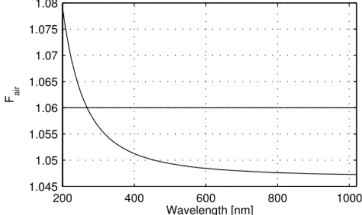
Figure 1 shows calculated King factors in the UV–Vis– NIR. For illustration, Fair equals 1.063 at λ=250 nm and 1.047 at λ=1 µm. The constant value of 1.06 leads to an error in the Rayleigh cross section of respectively 0.3 and 1.2 %; the impact on the retrieval of relatively low aerosol extinction coefficients is significant.
The AerGOM algorithm offers the choice to retrieve the neutral air density or to remove the contribution from the measured transmittanceTmeasby making use of ECMWF air
density profiles, as provided in the GOMOS residual extinc-tion files. The resulting transmissionT to be used for the data
inversion of all other species is given by
T (λ, rt)=Tmeas(λ, r
t)
Tair(λ, rt) ,
200 400 600 800 1000 1.045
1.05 1.055 1.06 1.065 1.07 1.075 1.08
F air
Wavelength [nm]
Figure 1.The wavelength-dependent King factorFair (Bodhaine
et al., 1999), together with the commonly used value of 1.06.
withTairthe transmittance by neutral air having SGDNair: Tair(λ, rt)=exp −Cair(λ)Nair(rt)
.
3.3 Aerosol extinction modelization 3.3.1 Frequently used models
Prior to the actual inversion of occultation measurements, little is known about the composition, size distribution and morphology of atmospheric particles. The use of Mie the-ory to model extinction spectra for data inversion purposes is therefore limited. In practice, it is usually preferred to rep-resent aerosol extinction or optical thickness spectra by a smooth analytical function with a small number of param-eters (which are to be fitted). The well-known Ångström empirical power law (β=Aλ−α) is a prime example. It is
however not versatile enough; researchers are often forced to make the coefficientsAandαwavelength dependent, an
ap-proach that seems rather arbitrary. In the current operational GOMOS Level 2 algorithm (IPFv6.01), a quadratic polyno-mial of wavelength (Eq. 1) is assumed for the aerosol SAOD. In the past, retrieval algorithms for other occultation instru-ments such as SAGE III (Thomason et al., 2007) and POAM III (Lumpe et al., 2002) were equipped with similar spectral laws for aerosol extinctionβaer; however they are often
ex-pressed as a function of the natural logarithm of wavelength:
βaer(λ)=c0+c1log(λ)+c2(log(λ))2.
The formalism can of course be extended to general polynomials of functions of wavelength. As an example, quadratic polynomials of inverse wavelength (λ−1) have
3.3.2 AerGOM aerosol spectral law implementation Inspecting Eq. (1), we see that, among the three fit parame-ters, onlyτaer(λref)represents a physical quantity. There are
two reasons for why this formalism is not optimal: (1) the three coefficients τaer, c1 andc2 have a different unit and
magnitude, giving rise to scaling problems during numerical inversion, and (2) during the spatial inversion from SAOD to local extinction values, it is not clear whether or not altitude regularization constraints on the coefficients c1 and c2 are
meaningful. The GOMOS IPFv6.01 algorithm, making use of this implementation, avoids the second point by inverting onlyτaer(λref)with altitude regularization. It is the main
rea-son why GOMOS aerosol extinction profiles exhibit strong oscillations for other wavelengths thanλref=500 nm.
The AerGOM solution consists of a fairly simple mathe-matical reformulation. The SAOD, modelled as an mth
de-gree polynomial of a function of wavelength f (λ), can be
expressed as a Lagrangian interpolation formula between a number of discrete SAOD values τ (λi) at different
wave-lengths:
τaer(λ)=
m+1
X
i=1
qi(λ)τaer(λi), (3)
with spectral base functions
qi(λ)=
m+1
Y
j6=i
f (λ)−f (λj) f (λi)−f (λj) .
For example, a quadratic polynomial of inverse wave-length is specified by the choice m=2 and three spectral base functions:
qi(λ)=
(λ−1−λ−j1)(λ−1−λ−k1) (λi−1−λ−j1)(λi−1−λ−k1),
with λi, λj and λk three different wavelengths that have
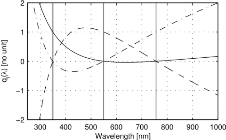
to be specified in advance. Examples of base functions are given in Fig. 2. The spectral behaviour of aerosols is now parametrized by three SAOD values, having the same order of magnitude and a direct physical meaning.
3.3.3 Aerosol spectral model: choice based on data The actual choice of aerosol spectral law should be based on its ability to model realistic spectra for particle popula-tions that are found in the atmosphere. By fitting measured or measurement-derived aerosol extinction spectra with a num-ber of candidate analytical extinction models, it is possible to single out one of these models that can be used in the AerGOM retrieval algorithm. We therefore consulted parti-cle size data derived from measurements that were performed by satellite instruments (SAGE II, CLAES and POAM), field campaign results (APE-THESEO; Airborne Platform
300 400 500 600 700 800 900 1000 −2
−1 0 1 2
Wavelength [nm]
q i
(
λ
) [no unit]
Figure 2.Aerosol spectral functionsq1(λ)(solid),q2(λ)(dashed)
andq3(λ)(dash-dot) for a quadratic polynomial of inverse
wave-length. The three predefined wavelengths areλ1=350 nm,λ2= 550 nm, andλ3=756 nm (vertical lines).
for Earth observation – contribution to the Third European Stratospheric Experiment on Ozone; Stefanutti et al., 2004) and many lidar and in situ instruments (Deshler et al., 2003). Measurements of different particle types were considered: (1) stratospheric sulfuric acid droplets, (2) polar stratospheric clouds (NAT: nitric acid trihydrate; STS: supercooled ternary solution; water ice) and (3) cirrus and subvisual cirrus clouds. Starting from published values of microphysical parame-ters (typically lognormal parameparame-ters for total number density, mode radius and distribution width), we simulated extinction spectra with a Mie code (assuming spherical particles). This of course requires the wavelength-dependent refractive in-dex of the particles under consideration. For pure-water ice these can be directly interpolated from tabulated data that were published by Warren (1984). The other particle types that are to be expected consist of binary and ternary solutions of sulfuric or nitric acid, of which the weight percentages (mainly driven by temperature) were obtained from theory: polar winter temperatures (Meilinger et al., 1995) as well as common stratospheric temperatures (Carslaw et al., 1997) were considered. From these weight percentages, the refrac-tive index was calculated with a code, published by Krieger et al. (2000), which is based on a generalized Lorentz– Lorenz equation for the refractive index. The various ways we calculated the refractive index for commonly encountered particle types in GOMOS data are summarized in Table 2.
Finally, the obtained spectra were fitted with a range of candidate spectral laws. Extinction and the logarithm of ex-tinction were fitted with second- and third-degree polynomi-als ofλ, 1/λ and log(λ). After comparison of the fit
qual-ity, the second-degree polynomial of inverse wavelength was singled out as a good versatile model for particle extinction spectra for the bulk of GOMOS measurements.
Table 2.The types of particles that are to be expected in the GOMOS data, with characteristics. The methods used to estimate composition (from temperature) and refractive index are also indicated.
Type State/morphology/composition Weight percentage Refractive index
Background Liquid/spherical, H2O/H2SO4 Carslaw et al. (1997) Krieger et al. (2000) Volcanic Liquid/spherical, H2O/H2SO4 Carslaw et al. (1997) Krieger et al. (2000)
Cirrus Solid/crystalline, H2O – Warren (1984)
NAT PSC Solid/amorphous, HNO3/H2O Meilinger et al. (1995) Krieger et al. (2000) STS PSC Liquid/spherical, H2O/H2SO4/HNO3 Meilinger et al. (1995) Krieger et al. (2000)
Ice PSC Solid/crystalline, H2O – Warren (1984)
Table 3.Stratospheric aerosols: lognormal particle size distribution parametersrm(mode radius) andσ (mode width), and aerosol
ex-tinctionβaerat 525 nm, representative of the period just before and after the Pinatubo eruption, at two different altitudes, in the 30– 50◦N latitude band. The data were derived from Figs. 4, 8 and 11
of Bauman et al. (2003). A few calculated refractive indices are also given.
Number rm σ βaer(525 nm)
in Fig. 3 (µm) (10−3km−1)
Altitude=18.5 km,T=217 K, H2SO4weight perc. = 78 % Refractive index=1.47 (400 nm), 1.46 (600 nm)
1 0.075 1.4 1
2 0.084 1.8 1
3 0.063 2.2 2
4 0.169 1.8 4
5 0.288 1.6 5
6 0.181 2.0 5
Altitude=26.5 km,T=223 K, H2SO4weight perc.=82 % Refractive index=1.48 (400 nm), 1.47 (600 nm)
7 0.092 1.2 0.05
8 0.151 1.4 0.4
9 0.127 1.8 2
10 0.230 1.6 4
11 0.288 1.6 8
12 0.346 1.6 12
width σ and 525 nm aerosol extinction βaero (respectively
Figs. 4, 8 and 11 in the paper) to the values in Table 3. Fur-thermore, stratospheric in situ data derived from impactor samples collected onboard an ER-2 aircraft (Pueschel et al., 1994) were used (see Table 4). In both cases, we assumed US76 temperatures at the considered altitudes and derived corresponding H2SO4weight percentages with the method
of Carslaw et al. (1997). Refractive indices were obtained with the method of Krieger et al. (2000). Finally, we calcu-lated the extinction spectra in Fig. 3 with a Mie code. Also shown are the fits with the quadratic polynomial of inverse wavelength; the correspondence is quite good.
3.4 Transmittance data
As mentioned before, the GOMOS IPFv6.01 processor uses exclusively SPA1 and SPA2 data for the retrieval of O3, NO2,
NO3 and aerosol extinction data products, while the SPB1
and SPB2 data are reserved for the retrieval of O2and H2O.
With respect to aerosol retrievals, this is regrettable; at longer wavelengths, the relative contribution of aerosol extinction is stronger (in the lower atmosphere) due to weaker air scatter-ing. Furthermore, anticipating future research, particle size distribution retrievals improve if the spectral range is larger (Fussen et al., 2002).
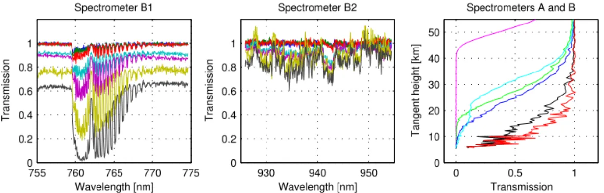
We therefore studied the possibility of exploiting SPB1 and SPB2 data in the AerGOM processor. Of course, care needs to be taken to avoid the use of wavelengths at which O2and H2O absorb. Figure 4 shows one way of doing this. It
is intuitively clear that the spectral ranges to the left and the right of the O2absorption band in the SPB1 data are useful
to extract aerosol extinction. On the other hand, it is far less obvious to define SPB2 spectral pixels that are free of H2O
absorption lines. The importance of these spectral regions is nevertheless clear when we observe the transmittance alti-tude profiles in the right panel of Fig. 4; in the lower strato-sphere and upper tropostrato-sphere (our main region of interest) a very useful range of transmittance is present in the SPB1 and SPB2 spectral bands while the SPA transmittance values have almost dropped to zero. For flexibility, the AerGOM processor offers the possibility to select SPA/SPB1/SPB2 spectral pixels at will. Due to the difficulty of finding SPB2 spectral pixels without H2O absorption, and the fact that
Aer-GOM is at present not able to perform H2O retrievals, SPB2
data are currently not selected for the retrievals. This situa-tion will likely change for future AerGOM data versions.
3.5 AerGOM spectral inversion
In comparison with the GOMOS processor, the AerGOM spectral inversion is conceptually much simpler. No separate differential method is used to derive NO2and NO3 SGDs.
Table 4.Stratospheric aerosols: bimodal lognormal particle size distribution parametersN0andN1(aerosol total number density),rm0and rm1(mode radius), andσ0andσ1(mode width), representative of the period just before and after the Pinatubo eruption. The data were obtained from impactor samples on an ER-2 aircraft and were published by Pueschel et al. (1994) (Table 1a). For optical calculations, we used a H2SO4weight percentage of 78 %, corresponding to a temperature of 217 K. Examples of refractive indices: 1.47 (400 nm), 1.46 (600 nm).
Number Date Latitude Longitude Altitude N0 rm0 σ0 N1 rm1 σ1
in Fig. 3 (km) (cm−3) (µm) (cm−3) (µm)
13 28 Feb 1991 40◦N 123◦W 18.3 1.0 0.1 1.8 0 0 0
14 14 Oct 1991 39◦N 123◦W 20.7 2.8 0.11 1.4 1.9 0.30 1.5
15 14 Oct 1991 66◦N 123◦W 18.5 2.8 0.13 1.6 0.6 0.55 1.2
16 2 Nov 1991 41◦N 107◦W 20.2 2.1 0.09 1.2 1.2 0.35 1.6
17 20 Mar 1992 48◦N 71◦W 20.0 0.4 0.09 1.5 1.8 0.46 1.7
1.5 2 2.5
0 1 2 3 4 5
x 10−3
1/λ [µm−1]
1 2
14 16 15
10 4 5 6
3 9
1.5 2 2.5
0 1 2 3 4 5 6 7x 10
−4
1/λ [µm−1]
7 13 8
1.5 2 2.5
0 0.002 0.004 0.006 0.008 0.01 0.012
1/λ [µm−1]
Extinction [km
−1]
17 11 12
Figure 3.Measured and fitted stratospheric sulfate aerosol extinction spectra for different aerosol size distributions. The three panels each cover a different extinction magnitude range. Crosses with dashed lines represent values derived from a SAGE II–CLAES climatology (red) and in situ impactor measurements (green). Also shown is the fit with the second-order polynomial of inverse wavelength (black solid lines). The numbers on the plots correspond to the data in Tables 3 and 4.
755 760 765 770 775
0 0.2 0.4 0.6 0.8 1
Wavelength [nm]
Transmission
Spectrometer B1
930 940 950
0 0.2 0.4 0.6 0.8 1
Wavelength [nm]
Transmission
Spectrometer B2
0 0.5 1
0 10 20 30 40 50
Transmission
Tangent height [km]
Spectrometers A and B
Figure 4.Examples of spectra (27 September 2004, 21.17◦S, 48.62◦E) for SPB1 (left) and SPB2 (middle) at tangent altitudes of (roughly)
15, 20, 25, 30, 35, 40 and 45 km (from bottom to top). Right panel: tangent altitude profiles of GOMOS transmittance for spectrometer A: 300 (magenta), 400 (green), 500 (blue), 600 nm (cyan); spectrometer B1 (black); B2 (red); the B1 and B2 profiles are very rough estimates of what can be expected; they are median values of the wings left and right of the B1 oxygen band, and the entire B2 spectrum respectively.
forward model, which now reads
T (rt, λ)=exp
"
−X
i
Ci(λ)Ni(rt)−
X
j
qj(λ)τaer(rt, λj))
#
.
The first term in the exponent indicates a summation over all gaseous species (O3, NO2and NO3, if Rayleigh scattering is
3.6 AerGOM spatial inversion
AerGOM performs a spatial inversion on all species simul-taneously. This allows the full use of all spectral inversion covariances between different species, which are discarded by the GOMOS IPFv6.01 processor. The importance of these covariances is crucial: using them in the spatial inversion sig-nificantly reduces the volume of the state space of possible solutions.
Spatial inversion of all species simultaneously is achieved by expressing the forward model as
Ntot=Gtotntot,
with Ntot a column vector containing all gas SGDs and
aerosol SAODs obtained from the spectral inversion, ntot a
column vector containing all local gas densities and aerosol extinction coefficients, and Gtot a matrix containing
opti-cal path lengths, similar to the ones that were discussed in Sect. 2.2.3.
Also here, to control the smoothness of the altitude pro-files, the linear inversion is performed with a Tikhonov regu-larization constraint. The merit functionMto be minimized
reads
M=[Ntot−Gtotntot]TSN,−1tot[Ntot−Gtotntot] +nTtotHtotntot,
with Ntot here representing actual GOMOS-derived SGDs
and SAODs, SN,tot the associated total covariance matrix
that is formed by stacking together all covariance matrices (including off-diagonal elements) obtained from the spectral inversion, andHtotthe Tikhonov smoothing operator. The
so-lution is given by
ntot=Sn,totGtotT S−N,1totNtot,
with solution covariance matrix Sn,tot=
GT
totS−N,1totGtot+Htot
−1
. (4)
Care should be taken to properly scale Htot, since
atmo-spheric species profiles span several orders of magnitude. A natural scaling is provided by the unconstrained least-squares covariance matrix of the solution (obtained by putting the Tikhonov term in Eq. 4 to zero):
Sn,tot, LS=GTtotS−N,1totGtot
−1
=DRD, (5)
where we have also expressed the covariance matrix in terms of the diagonal standard deviation matrixDand the correla-tion matrixR. We then choose the regularization operator as follows:
Htot=LtotD−1
T
LtotD−1
,
Table 5.Summary of the main configuration settings for the Aer-GOM v1.0 processing.
Implementation Setting
Retrieved species O3, NO2, NO3, aerosols–clouds
Full covariance matrix (FCM) no
Top of atmosphere 120 km
Rayleigh scattering From ECMWF (P >1 hPa)
and MSIS90 (P <1 hPa)
τaer(λ) Quadratic polynomial of 1/λ
τaerparametrized at 350, 550, and 756 nm
Spectral windows selected 248.1–685 nm (SPA)
755–759.3 nm (SPB1) 770–775 nm (SPB1)
Tikhonov parametersµi Gases: 0.1
Aerosol extinction: 3
where it is understood that Ltot is a composite operator,
consisting of several first-difference operators Li (one for
each gas density and aerosol extinction profile), each one of them multiplied with its own regularization parameterµi.
The functionality of the applied scaling becomes clear when we rewrite the covariance matrix of the regularized solution (Eq. 4):
Sn,tot=DR−1+LTtotLtot
−1
D.
We then compare it with the least-squares covariance matrix (Eq. 5): the altitude smoothing operates directly on the cor-relation matrixR, which is properly scaled by definition. 3.7 Results
3.7.1 AerGOM processing
The entire 10-year GOMOS data set has been processed with the AerGOM algorithm. The specific configuration that was chosen, taking into account the required data quality and pro-cessing speed, is presented in Table 5. Notice specifically that for this first tentative processing the FCM method was not used because it is computationally expensive. Further-more, the Rayleigh contribution was not retrieved but com-puted and removed, using meteorological data together with the Rayleigh cross section (Eq. 2). Finally, SPB2 data were not used (since all wavelengths are affected by water vapour, a species that is currently not retrieved by AerGOM), while only the SPB1 spectral pixels outside the O2absorption band
were exploited.
−1 0 1 2 3 10
20 30 40
IPFv6.01 − 386 nm
Alt. [km]
−1 0 1 2 3 10
20 30 40
IPFv6.01 − 452 nm
Alt. [km]
−1 0 1 2 3 10
20 30 40
IPFv6.01 − 525 nm
Alt. [km]
β aero [10
−3 km−1]
−1 0 1 2 3 10
20 30 40
AerGOMv1.0 − 386 nm
Alt. [km]
−1 0 1 2 3 10
20 30 40
AerGOMv1.0 − 452 nm
Alt. [km]
−1 0 1 2 3 10
20 30 40
AerGOMv1.0 − 525 nm
Alt. [km]
β aero [10
−3 km−1]
−6 −5 −4 −3 10
20 30 40
AerGOMv1.0 − 386 nm
Alt. [km]
−6 −5 −4 −3 10
20 30 40
AerGOMv1.0 − 452 nm
Alt. [km]
−6 −5 −4 −3 10
20 30 40
AerGOMv1.0 − 525 nm
Alt. [km]
log
10(βaero [km −1])
Figure 5.A set of 115 randomly chosen GOMOS aerosol extinction profiles, evaluated at three wavelengths, for the two algorithms. Left column: IPFv6.01; middle column: AerGOM v1.0. Right column: AerGOM v1.0, base 10 logarithm of aerosol extinction.
300 400 500 600 700 −10
0 10 20
IPFv6.01 − 20 km
Ext. × 10 −4 [km −1 ]
300 400 500 600 700 −2
0 2 4
IPFv6.01 − 25 km
Ext. × 10 −4 [km −1 ]
300 400 500 600 700 −1
0 1 2 3
IPFv6.01 − 30 km
Ext. × 10 −4 [km −1 ] Wavelength [nm]
300 400 500 600 700 −10
0 10 20
AerGOMv1.0 − 20 km
300 400 500 600 700 −2
0 2 4
AerGOMv1.0 − 25 km
300 400 500 600 700 −1
0 1 2 3
AerGOMv1.0 − 30 km
Wavelength [nm]
Figure 6.Aerosol extinction spectra at altitudes 20, 25 and 30 km. The same data set as in Fig. 5 was used. Left column: IPFv6.01; right column: AerGOM v1.0.
3.7.2 A first look at the AerGOM results
A detailed validation will be presented in a companion paper (Robert et al., 2016). Here, we will present a qualitative eval-uation of the obtained AerGOM data by comparison with the IPFv6.01 products; visual inspection is sufficient to demon-strate the improvement.
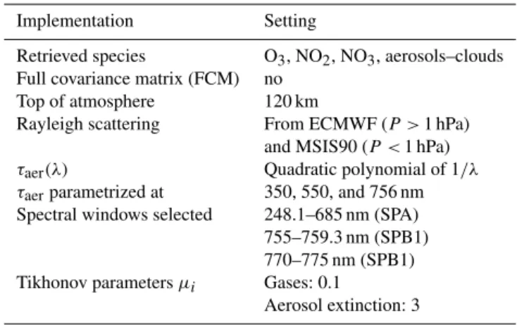
Figure 5 shows an ensemble of 115 randomly chosen aerosol extinction profiles (in a window from April 2002 to April 2005, between 60◦S and 60◦N), evaluated at three
wavelengths (386, 452 and 525 nm) using the assumed quadratic law. Clearly visible are the IPFv6.01 spurious os-cillations, which increase in amplitude for wavelengths far-ther away from the reference wavelength of 500 nm. As was anticipated, the situation improves dramatically for the Aer-GOM data.
We also observe a larger spread of the aerosol extinction profiles at lower altitudes (below about 20 km) for both re-trieval algorithms. The most important reason for this in-creased variability is not related to retrieval methodology but to the limited signal-to-noise (S/N) ratio of a stellar
0 200 400 600 800 1000 −5
0 5 10
x 10−4 IPFv6.01, z = 24 km, ρ = 0.095
Ext. [km
−1
]
0 200 400 600 800 1000
−5 0 5 10
x 10−4 AerGOMv1.0, z = 24 km, ρ = 0.296
Ext. [km
−1
]
0 200 400 600 800 1000
−2 0 2 4
x 10−4 IPFv6.01, z = 29 km, ρ = 0.056
Ext. [km
−1]
0 200 400 600 800 1000
−2 0 2 4
x 10−4 AerGOMv1.0, z = 29 km, ρ = 0.537
Ext. [km
−1]
0 200 400 600 800 1000
−1 0 1 2
x 10−4 IPFv6.01, z = 34 km, ρ = 0.050
Ext. [km
−1
]
Collocation no.
0 200 400 600 800 1000
−1 0 1 2
x 10−4 AerGOMv1.0, z = 34 km, ρ = 0.374
Ext. [km
−1
]
Collocation no.
Figure 7.A chronological series of aerosol extinction values at 386 nm, for 1152 GOMOS (blue) and SAGE II (red) collocations. From top to bottom: altitude=24, 29 and 34 km. Left column: IPFv6.01; right column: AerGOM v1.0. Correlation coefficientsρare also indicated in
the subplot titles.
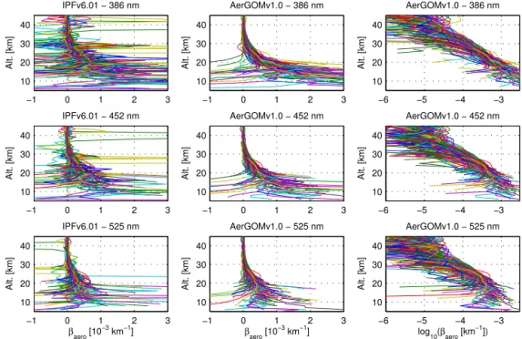
The same set of 115 profiles was used for the plots in Fig. 6, showing aerosol extinction spectra in the wavelength range from 300 to 750 nm at three different altitudes. Also here, much more consistent behaviour with fewer oscillations is exhibited by the AerGOM v1.0 data set. Notice the in-creased variability of extinction values at short wavelengths (below 400 nm), reflecting the larger retrieval errors due to the small aerosol–molecular extinction ratio at these wave-lengths. In particular, the spectral maxima between 300 and 400 nm should not be considered as physical features but re-sult from the lack of instrument sensitivity to aerosols.
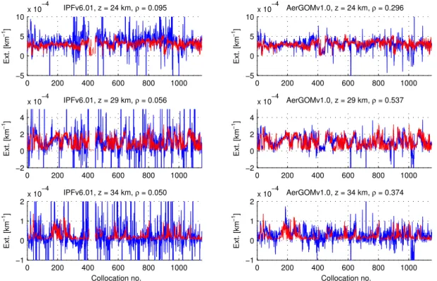
The correspondence between the IPFv6.01 and AerGOM data sets with SAGE II results is illustrated in Fig. 7. Shown are chronologically ordered aerosol extinction val-ues at 386 nm for collocated GOMOS–SAGE II occultation events (within a window of 500 km and 12 h), at three differ-ent altitudes spanning the middle stratosphere. On average, the IPFv6.01 data follow the SAGE II values closely but are very noisy. The amplitude of this noise decreases strongly in the AerGOM v1.0 series, and the overall agreement be-tween AerGOM and SAGE II values seems to be very good. This is confirmed when we inspect the correlation coeffi-cients (also given in Fig. 7), which are significantly larger for the SAGE II–AERGOM case, even up to 1 order of mag-nitude at 29 km. It should be mentioned that aerosol extinc-tion retrievals at the small wavelength of 386 nm are of lim-ited quality due to the much larger contribution of neutral
density Rayleigh scattering to the total extinction. For exam-ple, typical SAGE II aerosol extinction retrieval errors are 22 % (24 km), 32 % (29 km) and 45 % (34 km), with similar or larger numbers for GOMOS–AerGOM retrievals, depend-ing on the magnitude and temperature of the used star. This limited aerosol information content manifests itself in cor-relation coefficients that are still very modest. Nevertheless, the much higher SAGE II–AerGOM coefficients demonstrate the improvement with respect to IPFv6.01.
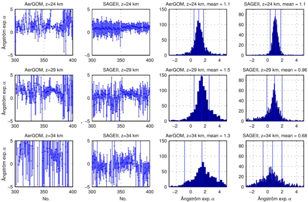
Coming back to the aerosol extinction spectra in Fig. 6 we observe that, while the AerGOM results look more consistent than the IPF ones, quite a large spectral variability (roughly speaking, the slope of the spectra with respect to wavelength) is still present. At first sight, this seems to suggest a strong variability of particle size distributions. This contradicts the fact that the considered period (2002–2005) was remarkably stable and free from major volcanic eruptions (only back-ground aerosols). However, the observed spectral variation is just caused by instrument noise, and the associated extinc-tion error bars are quite large. To demonstrate this, we have fitted an Ångström power law to the 386, 425 and 525 nm AerGOM extinction values (evaluated at these wavelengths using the assumed quadratic polynomial of inverse wave-length), as well as the SAGE II values for comparison:
300 350 400 −5
0 5
AerGOM, z=24 km
Angström exp.
α
300 350 400
−5 0 5
AerGOM, z=29 km
Angström exp.
α
300 350 400
−5 0 5
AerGOM, z=34 km
Angström exp.
α
No.
300 350 400
−5 0 5
SAGEII, z=24 km
300 350 400
−5 0 5
SAGEII, z=29 km
300 350 400
−5 0 5
SAGEII, z=34 km
No.
−2 0 2 4
0 50 100 150
AerGOM, z=24 km, mean = 1.1
−2 0 2 4
0 50 100 150
AerGOM, z=29 km, mean = 1.5
−2 0 2 4
0 50 100 150
AerGOM, z=34 km, mean = 1.3
Angström exp. α
−2 0 2 4
0 20 40 60 80
SAGEII, z=24 km, mean = 1.1
−2 0 2 4
0 20 40 60 80
SAGEII, z=29 km, mean = 0.96
−2 0 2 4
0 20 40 60 80
SAGEII, z=34 km, mean = 0.68
Angström exp. α
o o
o
o
o
o
Figure 8.Ångström exponents (AEs) derived from GOMOS–AerGOM and SAGE II data. The same data as for Fig. 7 were used. First two columns: 100 examples of AE for AerGOM and SAGE II at three different altitudes, with error bars. Third and fourth column: AE histograms for the full set of 1152 GOMOS–SAGE II collocations at three different altitudes. Vertical lines represent the error-weighted mean of the distribution (central line), and the median experimental error bars of the AE. The AE weighted mean is also indicated in the subplot titles.
withAa constant and αthe Ångström exponent (AE) that
describes the spectral shape. The extinction retrieval errors were taken into account. Results are shown in Fig. 8 at three different altitudes. We immediately see that the variability of the AE is for the most part buried in the experimental error and is therefore statistically not significant. The histograms in the figure for the full GOMOS–SAGE II collocation data set confirm this finding: the statistical spread of the AE dis-tributions falls largely within the limits of the experimental error. The findings are valid for AerGOM as well as SAGE II.
4 Conclusions
The GOMOS aerosol extinction profiles produced by the official IPFv6.01 algorithm are of good quality around the 500 nm reference wavelength, but they show pathological be-haviour in other spectral regions. This finding hinted at a con-ceptual error in the algorithm, instead of a lack of informa-tion in the GOMOS data. Within the framework of the Aer-GOM project, a new algorithm was developed that has some similarities with the IPF code but is equipped with two fun-damentally different concepts: an improved aerosol spectral law and a full spatial inversion that does not discard retrieval covariances between species. Additionally, a more accurate Rayleigh scattering cross section and air refractive index has been implemented. The spectral range has been increased by
the possibility to use SPB1 and SPB2 spectral measurements (although only SPB1 data have been selected for the first data processing presented in this paper).
The entire GOMOS 10-year mission data set has been pro-cessed, and the resulting Level 2 product files (containing al-titude profiles for aerosol extinction and gas densities, with error estimates) have been stored as the AerGOM v1.0 data set. An initial inspection of the obtained results shows that the pathological behaviour of the aerosol profiles at wave-lengths far from the 500 nm reference is severely reduced. Furthermore, a coarse comparison of GOMOS–SAGE II co-locations shows much better agreement for AerGOMv1.0 than for IPFv6.01 at these wavelengths. Since algorithm de-velopment forms the subject of this paper, a detailed vali-dation study of the aerosol extinction product has been pre-sented in a separate companion paper (Robert et al., 2016). Validation of the other products (O3, NO2, NO3) will be
car-ried out in the future. Finally, it should be mentioned that a new algorithm has been developed for the inversion of aerosol–cloud extinction spectra to particle size distributions. We will also discuss this algorithm in a separate publication.
5 Data availability
and can be obtained by contacting Christine Bingen ([email protected]).
Acknowledgements. The AerGOM project was financed by the
European Space Agency (contract number 22022/OP/I-OL). Addi-tional research was supported by a Marie Curie Career Integration Grant within the 7th European Community Framework Programme under grant agreement no. 293560, the European Space Agency within the Aerosol_CCI project of the Climate Change Initiative and the Belgian Space Science Office (BELSPO) through the “Chercheur Supplémentaire” programme.
Edited by: O. Torres
Reviewed by: two anonymous referees
References
Bates, D.: Rayleigh scattering by air, Planet. Space Sci., 32, 785– 790, 1984.
Bauman, J. J., Russell, P. B., Geller, M. A., and Hamill, P.: A strato-spheric aerosol climatology from SAGE II and CLAES mea-surements: 2. Results and comparisons, 1984–1999, J. Geophys. Res., 108, 4383, doi:10.1029/2002JD002993, 2003.
Bernath, P. F., McElroy, C. T., Abrams, M. C., Boone, C. D., Butler, M., Camy-Peyret, C., Carleer, M., Clerbaux, C., Coheur, P.-F., Colin, R., DeCola, P., DeMazière, M., Drummond, J. R., Du-four, D., Evans, W. F. J., Fast, H., Fussen, D., Gilbert, K., Jen-nings, D. E., Llewellyn, E. J., Lowe, R. P., Mahieu, E., Mc-Conell, J. C., McHugh, M., McLeod, S. D., Michaud, R., Mid-winter, C., Nassar, R., Nichitiu, F., Nowlan, C., Rinsland, C. P., Rochon, Y. J., Rowlands, N., Semeniuk, K., Simon, P., Skel-ton, R., Sloan, J. J., Soucy, M. A., Strong, K., Tremblay, P., Turnbull, D., Walker, K. A., Walkty, I., Wardle, D. A., Wehrle, V., Zander, R., and Zou, J.: Atmospheric Chemistry Experiment (ACE): Mission overview, Geophys. Res. Lett., 32, L15S01, doi:10.1029/2005GL022386, 2005.
Bertaux, J., Kyrölä, E., and Wehr, T.: Stellar occultation technique for atmospheric ozone monitoring: GOMOS on Envisat, Earth Obs. Quarterly, 67, 17–20, 2000.
Bertaux, J. L., Kyrölä, E., Fussen, D., Hauchecorne, A., Dalaudier, F., Sofieva, V., Tamminen, J., Vanhellemont, F., Fanton d’Andon, O., Barrot, G., Mangin, A., Blanot, L., Lebrun, J. C., Pérot, K., Fehr, T., Saavedra, L., Leppelmeier, G. W., and Fraisse, R.: Global ozone monitoring by occultation of stars: an overview of GOMOS measurements on ENVISAT, Atmos. Chem. Phys., 10, 12091–12148, doi:10.5194/acp-10-12091-2010, 2010.
Bodhaine, B. A., Wood, N. B., Dutton, E. G., and Slusser, J. R.: On Rayleigh Optical Depth Calculations, J. Atmos. Ocean. Tech., 16, 1854–1861, 1999.
Carslaw, K. S., Peter, T., and Clegg, S. L.: Modeling the composi-tion of liquid stratospheric aerosols, Rev. Geophys., 35, 125–154, 1997.
Chu, W., McCormick, M., Lenoble, J., Brogniez, C., and Pruvost, P.: SAGE II inversion algorithm, J. Geophys. Res., 94, 8339–8351, 1989.
Deshler, T., Hervig, M. E., Hofmann, D. J., Rosen, J. M., and Liley, J. B.: Thirty years of in situ stratospheric aerosol size
distribution measurements from Laramie, Wyoming (41◦N),
us-ing balloon-borne instruments, J. Geophys. Res., 108, 4167, doi:10.1029/2002JD002514, 2003.
Edlén, B.: The refractive index of air, Metrologia, 2, 71–80, 1966. Fussen, D., Vanhellemont, F., and Bingen, C.: Remote Sensing of
the Earth’s atmosphere by the spaceborne Occultation Radiome-ter, ORA: final inversion algorithm, Appl. Optics, 40, 941–948, 2001.
Fussen, D., Vanhellemont, F., and Bingen, C.: Optimal spectral in-version of atmospheric radiometric measurements in the near-UV to near-IR range: A case study, Opt. Express, 10, 70–82, 2002.
Krieger, U. K., Mössinger, J. C., Luo, B., Weers, U., and Peter, T.: Measurement of the refractive indices of H2SO4-HNO3-H2O solutions to stratospheric temperatures, Appl. Optics, 39, 3691– 3703, 2000.
Kyrölä, E., Tamminen, J., Leppelmeier, G., Sofieva, V., Hassinen, S., Bertaux, J., Hauchecorne, A., Dalaudier, F., Cot, C., Korablev, O., Fanton d’Andon, O., Barrot, G., Mangin, A., Theodore, B., Guirlet, M., Etanchaud, F., Snoeij, P., Koopman, R., Saavedra, L., Fraisse, R., Fussen, D., and Vanhellemont, F.: GOMOS on Envisat – an overview, Adv. Space Res., 33, 1020–1028, 2004. Kyrölä, E., Tamminen, J., Sofieva, V., Bertaux, J. L., Hauchecorne,
A., Dalaudier, F., Fussen, D., Vanhellemont, F., Fanton d’Andon, O., Barrot, G., Guirlet, M., Mangin, A., Blanot, L., Fehr, T., Saavedra de Miguel, L., and Fraisse, R.: Retrieval of atmospheric parameters from GOMOS data, Atmos. Chem. Phys., 10, 11881– 11903, doi:10.5194/acp-10-11881-2010, 2010.
Kyrölä, E., Blanot, L., Tamminen, J., Sofieva, V., Bertaux, J.-L., Hauchecorne, A., Dalaudier, F., Fussen, D., Vanhellemont, F., Fanton d’Andon, O., and Barrot, G.: GOMOS-Algorithm The-oretical Basis Document, version 3.0, Tech. rep., ESA, 2012. Lenoble, J.: Atmospheric Radiative Transfer – Studies in
Geophys-ical Optics and Remote Sensing, A. Deepak Publishing, Hamp-ton, VA, USA, 1993.
Lucke, R. L., Korwan, D. R., Bevilacqua, R., Hornstein, J. S., Shet-tle, E. P., Chen, D. T., Daehler, M., Lumpe, J. D., Fromm, M. D., Debrestian, D., Neff, B., Squire, M., König-Langlo, G., and Davies, J.: The Polar Ozone and Aerosol Measurement (POAM) III instrument and early validation results, J. Geophys. Res., 104, 18785–18799, 1999.
Lumpe, J. D., Bevilacqua, R. M., Hoppel, K. W., and Randall, C. E.: POAM III retrieval algorithm and error analysis, J. Geophys. Res.-Atmos, 107, 4575, doi:10.1029/2002JD002137, 2002. McElroy, C. T., Nowlan, C. R., Drummond, J. R., Bernath, P. F.,
Barton, D. V., Dufour, D. G., Midwinter, C., Hall, R. B., Ogyu, A., Ullberg, A., Wardle, D. I., Kar, J., Zou, J., Nichitiu, F., Boone, C. D., Walker, K. A., and Rowlands, N.: The ACE-MAESTRO instrument on SCISAT: description, performance, and prelimi-nary results, Appl. Optics, 46, 4341–4356, 2007.
Meilinger, S. K., Koop, T., Luo, B. P., Huthwelker, T., Carslaw, K. S., Krieger, U., Crutzen, P. J., and Peter, T.: Size-dependent stratospheric droplet composition in leewave temperature fluctu-ations and their potential role in PSC freezing, Geophys. Res. Lett., 22, 3031–3034, 1995.
Peck, E. R. and Reeder, K.: Dispersion of air, JJ. Opt. Soc. Am., 62, 958–962, 1972.
Pueschel, R., Russell, P., Allen, D., Ferry, G., Snetsinger, K., Liv-ingston, J., and Verma, S.: Physical and optical properties of the Pinatubo volcanic aerosol: aircraft observations with impactors and a Sun-tracking photometer, J. Geophys. Res., 99, 12915– 12922, 1994.
Robert, C. É., Bingen, C., Vanhellemont, F., Mateshvili, N., Dekem-per, E., Tétard, C., Fussen, D., Bourassa, A., and Zehner, C.: AerGOM, an improved algorithm for stratospheric aerosol ex-tinction retrieval from GOMOS observations – Part 2: Intercom-parisons, Atmos. Meas. Tech., 9, 4701–4718, doi:10.5194/amt-9-4701-2016, 2016.
Sofieva, V. F., Kan, V., Dalaudier, F., Kyrölä, E., Tamminen, J., Bertaux, J.-L., Hauchecorne, A., Fussen, D., and Vanhellemont, F.: Influence of scintillation on quality of ozone monitoring by GOMOS, Atmos. Chem. Phys., 9, 9197–9207, doi:10.5194/acp-9-9197-2009, 2009.
Sofieva, V. F., Vira, J., Kyrölä, E., Tamminen, J., Kan, V., Dalaudier, F., Hauchecorne, A., Bertaux, J.-L., Fussen, D., Vanhelle-mont, F., Barrot, G., and Fanton d’Andon, O.: Retrievals from GOMOS stellar occultation measurements using characteriza-tion of modeling errors, Atmos. Meas. Tech., 3, 1019–1027, doi:10.5194/amt-3-1019-2010, 2010.
SPARC: Report no. 4: Assessment of Stratospheric Aerosol Prop-erties (ASAP), edited by: Thomason, L. and Peter, T., Re-port WCRP-124 / WMO/TD-No. 1295, WMO/ICSU/IOC World Climate Research Programme, http://www.sparc-climate.org/ publications/sparc-reports/, 2006.
Stefanutti, L., MacKenzie, A. R., Santacesaria, V., Adriani, A., Balestri, S., Borrmann, S., Khattatov, V., Mazzinghi, P., Mitev, V., Rudakov, V., Schiller, C., Toci, G., Volk, C. M., Yushkov, V., Flentje, H., Kiemle, C., Redaelli, G., Carslaw, K. S., Noone, K., and Peter, T.: The APE-THESEO Trop-ical Campaign: An Overview, J. Atmos. Chem., 48, 1–33, doi:10.1023/B:JOCH.0000034509.11746.b8, 2004.
Tamminen, J., Kyrölä, E., Sofieva, V. F., Laine, M., Bertaux, J.-L., Hauchecorne, A., Dalaudier, F., Fussen, D., Vanhellemont, F., Fanton-d’Andon, O., Barrot, G., Mangin, A., Guirlet, M., Blanot, L., Fehr, T., Saavedra de Miguel, L., and Fraisse, R.: GOMOS data characterisation and error estimation, Atmos. Chem. Phys., 10, 9505–9519, doi:10.5194/acp-10-9505-2010, 2010.
Thomason, L. W., Poole, L. R., and Randall, C. E.: SAGE III aerosol extinction validation in the Arctic winter: comparisons with SAGE II and POAM III, Atmos. Chem. Phys., 7, 1423– 1433, doi:10.5194/acp-7-1423-2007, 2007.
Thomason, L. W., Moore, J. R., Pitts, M. C., Zawodny, J. M., and Chiou, E. W.: An evaluation of the SAGE III version 4 aerosol ex-tinction coefficient and water vapor data products, Atmos. Chem. Phys., 10, 2159–2173, doi:10.5194/acp-10-2159-2010, 2010. Vanhellemont, F., Fussen, D., Bingen, C., Kyrölä, E., Tamminen, J.,
Sofieva, V., Hassinen, S., Verronen, P., Seppälä, A., Bertaux, J. L., Hauchecorne, A., Dalaudier, F., Fanton d’Andon, O., Barrot, G., Mangin, A., Theodore, B., Guirlet, M., Renard, J. B., Fraisse, R., Snoeij, P., Koopman, R., and Saavedra, L.: A 2003 strato-spheric aerosol extinction and PSC climatology from GOMOS measurements on Envisat, Atmos. Chem. Phys., 5, 2413–2417, doi:10.5194/acp-5-2413-2005, 2005.
Vanhellemont, F., Fussen, D., Dodion, J., Bingen, C., and Mateshvili, N.: Choosing a suitable analytical model for aerosol extinction spectra in the retrieval of UV/visible satel-lite occultation measurements, J. Geophys. Res., 111, D23203, doi:10.1029/2005JD006941, 2006.
Vanhellemont, F., Tetard, C., Bourassa, A., Fromm, M., Dodion, J., Fussen, D., Brogniez, C., Degenstein, D., Gilbert, K. L., Turn-bull, D. N., Bernath, P., Boone, C., and Walker, K. A.: Aerosol extinction profiles at 525 nm and 1020 nm derived from ACE imager data: comparisons with GOMOS, SAGE II, SAGE III, POAM III, and OSIRIS, Atmos. Chem. Phys., 8, 2027–2037, doi:10.5194/acp-8-2027-2008, 2008.
Vanhellemont, F., Fussen, D., Mateshvili, N., Tétard, C., Bingen, C., Dekemper, E., Loodts, N., Kyrölä, E., Sofieva, V., Tamminen, J., Hauchecorne, A., Bertaux, J.-L., Dalaudier, F., Blanot, L., Fan-ton d’Andon, O., Barrot, G., Guirlet, M., Fehr, T., and Saave-dra, L.: Optical extinction by upper tropospheric/stratospheric aerosols and clouds: GOMOS observations for the period 2002– 2008, Atmos. Chem. Phys., 10, 7997–8009, doi:10.5194/acp-10-7997-2010, 2010.